Vol. 41
No. 4
IPSJ Journal
Apr. 2000
Regular Paper
“Approximate Zero-points” of Real Univariate Polynomial
with Large Error Terms
Akira Terui† and Tateaki Sasaki†
Let P (x) be a given real univariate polynomial and let P̃ (x) = P (x) + ∆(x), where ∆(x) is
the sum of error terms, that is, a polynomial with small real unknown but bounded coefficients.
We first consider specifying the “existence domain” of the values of P̃ (x), or the domain in
which the value of P̃ (x) exists for any real number x, by the coefficient bounds for ∆(x),
and then introduce a concept of an “approximate real zero-point” of P̃ (x). We present a
practical method for estimating the existence domain of zero-points of P̃ (x) by applying
Smith’s celebrated theorem. We next consider counting the number of real zero-points of
P̃ (x). If all the zero-points are sufficiently far apart from each other, the number of real
zero-points of P̃ (x) is the same as that of P (x), and we derive a condition for which we can
assert that P (x) and P̃ (x) have the same number of real zero-points. We calculate the actual
number of real zero-points by Sturm’s method, which encounters the so-called small leading
coefficient problem. For this problem, we show that, under some conditions, small leading
terms can be discarded. Furthermore, we investigate four methods for evaluating the effect
of error terms on the elements of the Sturm sequence.
points can exist. Therefore, in this paper, we introduce a concept of an “approximate real zeropoint” by defining a minimal interval outside of
which no real zero-points can exist. Although
the existence domains of real zero-points can be
calculated rigorously, we propose methods for
calculating them approximately and efficiently
by using Smith’s theorem on the error bounds
of zero-points of a polynomial 11) .
Next, we consider calculation of the number
of real zero-points of an approximate polynomial by Sturm’s method. If all the zero-points
are single and well separated, the number of real
zero-points is definite unless some error term
is quite large, although the positions of zeropoints are changed by the error terms. However, in the calculation of the Sturm sequence,
the leading coefficient of some element may become too small to determine whether it is equal
to zero or not. Since the sign of the leading
coefficient in the Sturm sequence is essential in
determining the number of real zero-points, this
is a serious problem. Our answer to it is that,
under some conditions, we may discard the
small leading term and continue further calculation of the Sturm sequence. Shirayanagi and
Sekigawa 10) also attacked this problem, and
proposed an interval arithmetic method with
zero rewriting. We will investigate the Sturm
sequence with interval coefficients in Section 5.
In Section 2, we investigate the existence domains of the values of a real approximate poly-
1. Introduction
In traditional computer algebra on polynomials, we usually assume that the coefficients of
polynomials are given rigorously by integers, rational numbers, or algebraic numbers, and that
manipulation on the polynomials is also exact.
However, in many practical applications or realworld problems, the coefficients contain errors;
that is, polynomials have “error terms.” In
such cases, many of the traditional algorithms
in computer algebra break down.
This paper considers the real zero-points of
a real univariate polynomial with error terms,
or “approximate polynomial,” where the coefficients of error terms can be much larger than
the machine epsilon εM . In fact, even if the initial errors in coefficients are as small as εM , the
errors can become much larger than εM after the
calculation. Furthermore, in approximate algebraic calculation, we handle polynomials with
perturbed terms that are much larger than εM
in general.
If a polynomial P (x) has error terms, we cannot draw the graph of function y = P (x); all
we can draw is the “existence domain” of P (x),
or the domain in which values of P (x) can exist. Similarly, in such a case, the positions of
its zero-points cannot be determined exactly;
all we can handle is the domains in which zero† Institute of Mathematics, University of Tsukuba
974
Vol. 41
No. 4
“Approximate Zero-points” of Real Univariate Polynomial
nomial, then define an approximate real zeropoint. In Section 3, we propose a practical
method for calculating the existence domains
of the zero-points of an approximate polynomial. In Section 4, on the assumption that the
polynomial does not have multiple or close zeropoints, we derive a sufficient condition for the
number of real zero-points not to be changed
by error terms. In Section 5, we propose and
investigate several methods for checking the effect of the error terms of a given polynomial on
the Sturm sequence.
2. Approximate Polynomials and Approximate Real Zero-points
Let P (x) be a given univariate polynomial
with real coefficients such that
(1)
P (x) = cn xn + · · · + c0 x0 ,
and let P̃ (x) be a real univariate polynomial
such that
P̃ (x) = P (x) + ∆(x),
(2)
where ∆(x) represents the sum of real “error
terms,” that is, a polynomial with unknown
small real coefficients. Hence, we know neither
P̃ (x) nor ∆(x); what we know usually is an
upper bound for each coefficient in ∆(x). Representing ∆(x) as
∆(x) = δn−1 xn−1 + · · · + δ0 x0 ,
(3)
we assume that we know upper bounds
εn−1 , . . . , ε0 such that
(4)
|δi | ≤ εi , i = n − 1, . . . , 0.
Throughout this paper, we write P̃ (x | δi =
εi (i = n − 1, . . . , 0)) to denote that the values
of δn−1 , . . . , δ0 in P̃ (x) are specified as δn−1 =
εn−1 , . . . , δ0 = ε0 , and so on.
2.1 Existence Domain of Values of
P̃ (x)
Supposing that the variable x is fixed to x0
and that δn−1 , . . . , δ0 are changed continuously
under the restrictions in Eq. (4); the value of
P̃ (x0 ) moves continuously inside an interval.
By changing x0 in R, we will have the minimal
domain outside of which there is no possibility
of the existence of the value of P̃ (x).
Definition 1 (existence domain) Let x0
be a real number and δi move continuously in
the whole interval [−εi , εi ] for i = 0, . . . , n − 1.
Define PU (x0 ) and PL (x0 ) as
(5)
PU (x0 ) = max P̃ (x0 ),
δi ∈[−εi ,εi ]
i=0,...,n−1
PL (x0 ) =
min
δi ∈[−εi ,εi ]
i=0,...,n−1
P̃ (x0 ).
(6)
975
By changing the value x0 in R, we obtain a
domain
(7)
{[PL (x), PU (x)] | x ∈ R}.
We call this domain the “existence domain of
P̃ (x).”
✷
The existence domain of P̃ (x) can be specified rigorously by using P (x).
Lemma 1 Let the value of δi in P̃ (x) be
changed continuously within the range [−εi , εi ],
while the values of δj ’s (j = i) are fixed, and, for
each real value of x, define PUi (x) and PLi (x)
as
(8)
PUi (x) = max P̃ (x),
δi ∈[−εi ,εi ]
PLi (x) =
min
δi ∈[−εi ,εi ]
Then, we have
PUi (x) =
PLi (x) =
P̃ (x).
(9)
P̃ (x | δi = εi )
if x ≥ 0 or i is even,
(10)
P̃ (x | δi = −εi )
if x ≤ 0 and i is odd,
P̃ (x | δi = −εi )
if x ≥ 0 or i is even,
(11)
P̃ (x | δi = εi )
if x ≤ 0 and i is odd.
Furthermore, for any real value x0 , P̃ (x0 ) moves
all the points inside [PLi (x0 ), PUi (x0 )].
Proof. Let x0 be any real number. We see that
−εi |x0 |i ≤ δi |x0 |i ≤ εi |x0 |i , and since δi |x0 |i
moves all the points inside [−εi |x0 |i , εi |x0 |i ], we
obtain the lemma.
✷
This lemma directly leads us to the following
theorem:
Theorem 2 Let the polynomials P (x) and
P̃ (x) be as above; then the functions PU (x) and
PL (x) in Eq. (7) are given as follows:
P̃ (x | δi = εi
(i = n − 1, . . . , 0))
for x ≥ 0,
PU (x) =
(12)
P̃
(x
|
δi = (−1)i εi
(i = n − 1, . . . , 0))
for x < 0,
P̃ (x | δi = −εi
(i = n − 1, . . . , 0))
for x ≥ 0,
(13)
PL (x) =
P̃
(x
|
δi = (−1)i+1 εi
(i = n − 1, . . . , 0))
for x < 0.
Furthermore, for any real number x0 , the
values of P̃ (x0 ) move all the points inside
✷
[PL (x0 ), PU (x0 )].
976
IPSJ Journal
PL (x)
PU (x)
Apr. 2000
PL (x)
PU (x)
PU (x)
ê
PU (x)
1
ê
ê
1
2
(a)
x
ê
ê
1
x
2
(b)
ê
1
PL (x)
ê
2
x
2
(c)
ê
x
PL (x)
(d)
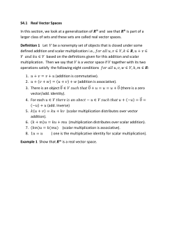
Fig. 1 Existence domain of an approximate real zero-point.
2.2 Approximate Real Zero-points and
Their Existence Domains
We first define a concept of “approximate real
zero-points” and their existence domains.
Definition 2 (approximate real zeropoint) A real number ζ is an “approximate
real zero-point of P̃ (x)” if there exist numbers εi ∈ [−εi , εi ] (i = n − 1, . . . , 0) such
that P̃ (ζ | δi = εi (i = n − 1, . . . , 0)) = 0.
Let [ζ1,1 , ζ1,2 ], . . . , [ζr,1 , ζr,2 ], with ζ1,1 ≤ ζ1,2 <
· · · < ζr,1 ≤ ζr,2 , be the set of all the approximate real zero-points of P̃ (x). Then, we call
each interval [ζi,1 , ζi,2 ], 1 ≤ i ≤ r, an “existence
domain” of the approximate real zero-point of
P̃ (x).
✷
Theorem 2 tells us that the existence domains
of all the approximate real zero-points can be
specified rigorously by drawing graphs of PL (x)
and PU (x). Suppose [ζ1 , ζ2 ] is an existence domain of an approximate real zero-point. Since
ζ1 and ζ2 are real zero-points of PU (x) and/or
PL (x), and since PL (x0 ) < PU (x0 ) for any real
number x0 , the graphs of PL (x) and PU (x)
around this interval can be classified into one
of the following four cases:
(a) PL (ζ1 ) = PU (ζ2 ) = 0, PL (x) < 0 for
ζ1 < x ≤ ζ2 , PU (x) > 0 for ζ1 ≤ x < ζ2 , and
there exists δ > 0 such that PL (ζ1 − x) > 0 and
PU (ζ2 + x) < 0 for any x ∈ [0, δ],
(b) PU (ζ1 ) = PL (ζ2 ) = 0, PU (x) > 0 for
ζ1 < x ≤ ζ2 , PL (x) < 0 for ζ1 ≤ x < ζ2 , and
there exists δ > 0 such that PU (ζ1 − x) < 0 and
PL (ζ2 + x) > 0 for any x ∈ [0, δ],
(c)
PL (ζ1 ) = PL (ζ2 ) = 0, PU (x) > 0 for
ζ1 ≤ x ≤ ζ2 , PL (x) < 0 for ζ1 < x < ζ2 , and
there exists δ > 0 such that PL (ζ1 − x) > 0 and
PL (ζ2 + x) > 0 for any x ∈ [0, δ],
(d) PU (ζ1 ) = PU (ζ2 ) = 0, PL (x) < 0 for
ζ1 ≤ x ≤ ζ2 , PU (x) > 0 for ζ1 < x < ζ2 , and
there exists δ > 0 such that PU (ζ1 − x) < 0 and
PU (ζ2 + x) < 0 for any x ∈ [0, δ].
Figure 1 illustrates these four cases conceptu-
ally. Cases (a) and (b) usually correspond to a
single zero-point, while Cases (c) and (d) correspond to multiple zero-points.
We now give a simple example of approximate real zero-points and their existence domains. We will see that one of the existence
domains is fairly wide, which indicates that the
concept of approximate zero-point is indispensable in handling polynomials with error terms.
Example 1 Let F (x, y) be
(14)
F (x, y) = x3 − x2 + y 2 .
We calculate a singular point of F (x, y) with
approximate arithmetic of precision εM = 1.0 ×
10−6 . First, let us calculate the discriminant
R(y) of F (x, y) with respect to x:
R(y) = res(F, dF/dx)
(15)
= 27y 4 − 4y 2 .
√
R(y) has zero-points at y = 0 and ±2 3/9. Assume
√ that we have calculated the value of y =
2 3/9 approximately as 0.384900. (Note that if
deg(R) ≥ 5 then use of approximate arithmetic
is necessary in general to solve R(y) = 0.) Let
P (x) and P̃ (x) be
P (x) = x3 − x2 + (0.384900)2 ,
(16)
P̃ (x) = P (x) + δ0 ,
−6
where |δ0 | ≤ 1.0 × 10 , and let us calculate
the approximate real zero-points of P̃ (x). From
Theorem 2, we have
PU (x) = x3 − x2 + 0.148149,
(17)
PL (x) = x3 − x2 + 0.148147.
PU (x) has a real zero-point at x −0.333334,
and PL (x) has real zero-points at x −0.333332, 0.665595, and 0.667738. From
Definition 2, the existence domains of approximate real zero-points of P̃ (x) are intervals [−0.333334, −0.333332], and [0.665595,
0.667738]. Therefore, with an approximate
arithmetic of precision εM = 1.0 × 10⁻⁶ , the
singular point (x0 , y0 ) of F (x, y) can be specified only vaguely as y0 ∈ [0.384899, 0.384901]
✷
and x0 ∈ [0.665595, 0.667738].
Vol. 41
No. 4
“Approximate Zero-points” of Real Univariate Polynomial
3. Bounding Existence Domains by
Using Smith’s Theorem
Although we have defined rigorously the existence domain of only real zero-points, we
present in this section a method for bounding
the existence domains of both real and complex
zero-points by means of discs in the complex
plane, because the method is common to both
of them.
A key to bounding existence domains is
Smith’s celebrated theorem. (For the proof, see
Smith 11) .)
Theorem 3 (Smith) Let P (x) be as
above. Let x1 , . . . , xn be n distinct numbers in
C and r1 , . . . , rn be defined as nP (xj )
rj = n
,
(18)
an k=1,=j (xj − xk ) j = 1, . . . , n.
Let Dj (1 ≤ j ≤ n) be a disc of radius
rj with its center at xj . Then, the union
D1 ∪ · · · ∪ Dn contains all the zero-points of
P (x). Furthermore, if a union D1 ∪ · · · ∪ Dm
(m ≤ n) is connected and does not intersect
with Dm+1 , . . . , Dn , then this union contains
exactly m zero-points.
✷
3.1 Single Zero-points
Without loss of generality, we assume that P
and P̃ are monic. Let ζ1 , . . . , ζn and ζ̃1 , . . . , ζ̃n
be the zero-points of P (x) and P̃ (x), respectively:
P (x) = (x − ζ1 )(x − ζ2 ) · · · (x − ζn ), (19)
P̃ (x) = (x − ζ̃1 )(x − ζ̃2 ) · · · (x − ζ̃n ). (20)
First, we consider the case in which ζ1 is a
single zero-point such that |ζ1 − ζj | εM for
j = 2, . . . , n. Let z1 , . . . , zn be approximate
values for ζ1 , . . . , ζn , respectively. (Actually,
we may determine z1 , . . . , zn by solving equation P (x) = 0 numerically, and hence approximately, with accuracy εM .) Using Theorem 3,
we can formally calculate the domain that contains ζ̃1 in C, as follows. Let R1 be
|P̃ (z1 )|
,
R1 = n · (21)
n
j=2 (z1 − zj )
then ζ̃1 is contained in the disc of radius R1 with
its center at z1 . Although we cannot calculate
P̃ (z1 ) explicitly, we have
|P̃ (z1 )| ≤ |P (z1 )| + |∆(z1 )|
n−1
(22)
≤ |P (z1 )| +
εj |z1 |j .
j=0
977
Therefore, R1 is bounded as
j
|P (z1 )| + n−1
j=0 εj |z1 |
.
(23)
R1 ≤ n ·
n
j=2 (z1 − zj )
In ordinary numerical computation, we calculate an error bound by the above formula with
εj = 0, which gives a good estimate such that
the magnitude of the error bound is only several times larger than the true error. Therefore,
we expect that the above formula gives a good
bound.
3.2 Multiple or Close Zero-points
Next, we consider the case of multiple or close
zero-points. Without loss of generality, let ζ1 · · · ζm (m ≤ n) and
√ assume that ζm+1 , . . . , ζn
satisfy |ζj − ζ1 | m εM for j = m + 1, . . . , n. In
this case, we cannot apply Eq. (23) directly, for
the following reason. Let z1 , . . . , zn be the same
as above and assume that we have calculated
them by a numerical method.
√ Then z1 , . . . , zm
usually satisfy |zj −z1 | m εM for j = 2, . . . , m;
hence, in Eq. (23), we have
n
n
(z1 − zj ) εM · (z
−
z
)
1
j .(24)
j=m+1
j=2
Therefore, if |∆(zi )| εM , an upper bound calculated by Eq. (23) will be an overestimate.
We determine z1 , . . . , zm so that the radius
R1 in Eq. (21) becomes as small as possible.
(The determination method is the same as that
described in the literature; for example, see
Iri 5) ; the only difference is that our setting of
error terms is different from the conventional
ones.) We express P (x) as
P (x) = (x − ζ1 ) · · · (x − ζm ) · Q(x). (25)
From our assumption, we have
n
(z1 − ζj )
Q(z1 ) =
j=m+1
n
(26)
(z1 − zj );
j=m+1
hence R1 defined by Eq. (21) can be approximated as follows:
n
j=1 (z1 − ζj ) + ∆(z1 )
R1 = n ·
(27)
n
j=2 (z1 − zj )
m
j=1 (z1 − ζj ) + ∆(z1 )/Q(z1 )
n·
.
m
j=2 (z1 − zj )
(28)
978
IPSJ Journal
If z1 , . . . , zm are distributed equally on a disc
of radius r with its center at (ζ1 + · · · + ζm )/m,
we have
m
(z1 − ζj ) ≈ r m ,
j=1
(29)
m
(z1 − zj ) = mr m−1 ,
j=2
Apr. 2000
4. Calculating the Number of Real
Zero-points of a Real Approximate
Polynomial
real zero-points of P̃ (x) is the same as that of
P (x) if the discriminant of P̃ , or res(P̃ , dP̃ /dx)
does not become zero for any values δn−1 , . . . , δ0
satisfying Eq. (4).
Proof. As the coefficients of P̃ (x) change continuously, the number of real zero-points of P̃ (x)
changes only if there exist δi ∈ [−εi , εi ] for
i = 0, . . . , n − 1 such that P̃ (x) has real multiple zero-points. Its contraposition shows the
validity of the theorem.
✷
Theorem 4 tells us that we can calculate the
number of real zero-points of an unknown polynomial P̃ (x) by calculating the number of the
real zero-points of P (x), so long as the discriminant res(P̃ , dP̃ /dx) does not become zero
for any values δn−1 , . . . , δ0 satisfying Eq. (4).
Therefore, we can check the definiteness of the
number of real zero-points by checking whether
or not res(P̃ , dP̃ /dx) becomes zero because of
the error terms.
4.2 Problem of Small Leading Coefficient in the Sturm Sequence
Below, the leading coefficient and the degree
of P (x) are denoted as lc(P ) and deg(P ), respectively. Let ζmax be the maximum of the
absolute values of real zero-points of P (x).
The p-norm of P (x), with P (x) given in
Eq. (1), is defined as
n
1/p
p
|ci |
,
P p =
(33)
If a real approximate polynomial has multiple or close zero-points, they may change significantly, or some real zero-points may become
complex, when the coefficients are changed
slightly. Therefore, it is not adequate to count
the number of real zero-points of a real approximate polynomial that may have multiple or
close zero-points. On the other hand, if a polynomial has only single zero-points, the number
of its real zero-points rarely changes, although
their positions may change considerably, when
the coefficients are changed slightly. In this section, we focus on calculating the number of real
zero-points of a real approximate polynomial
containing only single zero-points.
4.1 Sufficient Condition for Fixing the
Number of Real Zero-points
We first derive a sufficient condition for asserting that P (x) and P̃ (x) have the same number of real zero-points.
Theorem 4 Let P (x) and P̃ (x) be as in
Eqs. (1) and (2), respectively. The number of
p = 1, 2, . . . , ∞.
In this paper, we use the 2-norm for polynomials.
Assuming that P (x) and P̃ (x) satisfy the condition in Theorem 4, P 2 1, and P̃ 2 1,
let us consider calculation of the number of real
zero-points of P̃ (x) by application of Sturm’s
famous method to P (x). Sturm’s theorem is as
follows (for the proof, see Cohen 3) , for example):
Theorem 5 (Sturm) Let P (x) be a real
square-free polynomial of degree n, and define
a polynomial sequence (the Sturm sequence)
(34)
(P0 (x), P1 (x), . . . , Pn (x))
as
P = P (x),
0
d
P (x),
P1 = dx
(35)
=
−rem(P
P
i
i−2 , Pi−1 )
for i = 2, . . . , n,
where rem(Pi−2 , Pi−1 ) denotes the remainder of
Pi−2 divided by Pi−1 . For a real number x, let
N (x) be the number of sign changes, counting
and Eq. (28) can be evaluated as
rm + C
R1 n ·
,
(30)
mr m−1
where C = |∆(z1 )/Q(z1 )|. We can almost minimize the magnitude of R1 by setting r as
(31)
r = m (m − 1)C.
With the above consideration, we calculate an
upper bound for R1 as follows:
( 1 ) Calculate r from Eq. (31).
( 2 ) Let β = (ζ1 + · · · + ζm )/m and
(32)
zj = β + r exp(2πji/m)
for j = 1, . . . , m. The approximate values z1 , . . . , zm are distributed equally on
a disc of radius r with its center at β.
( 3 ) Substitute z1 , . . . , zm into Eq. (23) to obtain a rigorous bound of R1 .
i=1
Vol. 41
No. 4
“Approximate Zero-points” of Real Univariate Polynomial
from the left to the right without counting zeros, in the sequence (34), and let s and t be real
numbers satisfying s < t. Then, the number of
the real zero-points of P in the interval [s, t] is
equal to N (s) − N (t).
✷
Note that we can calculate the number of all
the real zero-points of P by putting s = −∞
and t = ∞ in Theorem 5. In the following, the
zeros of the Sturm sequence and its modifications are not counted as sign changes.
Consider calculation of the Sturm sequence
of P (x) by means of floating-point arithmetic.
During the calculation, we may encounter the
leading coefficient problem: (1) it is hard for us
to decide whether or not a very small leading
coefficient is equal to zero, and (2) the division
by a polynomial by a small leading coefficient
will cause large cancellation errors in the coefficients of the remainder polynomial.
Let P , s, and t be the same as in Theorem 5.
A Sturm sequence of P with Pn ≡ (constant) =
0 has the following properties (for example, see
Cohen 3) ):
1◦
For any real number x, consecutive elements Pi−1 (x) and Pi (x) do not simultaneously become zero.
If Pj (x) = 0 for some j (1 ≤ j < n) and
2◦
x ∈ R, then we have Pj−1 (x)Pj+1 (x) <
0.
Pn has no real zero-point.
3◦
With Property 1◦ , we can calculate the number
of sign changes by investigating each Pi separately. Let Pj (xj ) = 0 for some xj ∈ R; then
Property 2◦ means that Pj−1 and Pj+1 have
no zero-point in the neighborhood of x = xj .
Property 3◦ is trivial in our case, because Pn =
(constant), but it is not trivial for the general
Sturm sequence. The above three properties
are sufficient for determining the number of real
zero-points, and a sequence that has those properties is called a general Sturm sequence.
We note that the sign change of Pj (x) at
x = xj , j ≥ 1, does not affect the number of
sign changes in the sequence (34); the value of
N (x) changes only when the evaluation point x
passes a real zero-point of P0 (x) (= P (x)). Furthermore, we can prove the following property
of the Sturm sequence:
Lemma 6 Let P (x) and P0 , . . . , Pn be the
same as in Theorem 5, and assume that Pk (x) =
0 (1 < k < n) at x = xk,1 , . . . , xk,lk , where
lk < deg(Pk ) and |xk,j | > ζmax for j = 1, . . . , lk .
Define Pk (x) as
979
Pk (x)
, (36)
(x − xk,1 ) · · · (x − xk,lk )
and let s and t be real numbers satisfying s < t.
For real number x, let N (x) be the same as in
Theorem 5, and let Nk (x) be the numbers of
sign changes in the sequence
(P0 (x), . . . , Pk−1 (x),
(37)
Pk (x), Pk+1 (x), . . . , Pn (x)).
Then we have
(38)
Nk (s) − Nk (t) = N (s) − N (t).
That is, Nk (s) − Nk (t) is equal to the number
of real zero-points of P (x) in the interval [s, t].
Proof. Property 1◦ assures us that there exists
a small positive number δ such that [xk,j1 − δ,
xk,j1 + δ] ∩ [xk,j2 − δ, xk,j2 + δ] = ∅ for 1 ≤
j1 < j2 ≤ lk and Pk±1 (x) = 0 for any x ∈
[xk,j − δ, xk,j + δ]. We show Nk (x) = N (x)
for any x ∈ [xk,j − δ, xk,j + δ]. Consider
a case in which dPk /dx < 0 at x = xk,1 ,
Pk−1 (xk,1 ) > 0, and Pk+1 (xk,1 ) < 0. Property 2◦ says that the sequence of signs of
polynomials (Pk−1 (x), Pk (x), Pk+1 (x)) at x =
xk,1 − δ, x = xk,1 and x = xk,1 + δ are
(+, +, −), (+, 0, −) and (+, −, −), respectively;
hence the number of sign changes of the sequence (Pk−1 (x), Pk (x), Pk+1 (x)) is equal to 1
for any x ∈ [xk,1 − δ, xk,1 + δ]. Now, assume that Pk (x) > 0 for x ∈ [xk,1 − δ, xk,1 +
δ]; then the sequence of signs of polynomials
(Pk−1 (x), Pk (x), Pk+1 (x)) is (+, +, −) for any
x ∈ [xk,1 − δ, xk,1 + δ]. Therefore, we have
Nk (x) = N (x) for any x ∈ [xk,1 − δ, xk,1 + δ].
The other cases can be proved similarly.
✷
Theorem 7 Assume the same hypotheses
as in Lemma 6, and define a polynomial sequence
(P0 (x), . . . , Pk−1 (x), Pk (x), . . . , Pn (x)) (39)
as
Pk (x)
,
Pk =
(x − xk,1 ) · · · (x − xk,lk )
(40)
Pk+1
= −rem(Pk−1 , Pk ),
P
=
−rem(P
,
P
)
i
i−2
i−1
for i = k + 2, . . . , n ,
where deg(Pn ) = 0. For a real number x, let
N (x) be the number of sign changes in the
sequence (39), and let s and t be real numbers
satisfying s < t. Then, the number of real zeropoints of P (x) in the interval [s, t] is equal to
N (s) − N (t).
Proof. From Lemma 6, we need not consider
xk,1 , . . . , xk,lk for calculating the number of
real zero-points of P (x). Let xk be any zeropoint of Pk ; hence Pk−1 (xk ) = 0. Then,
(xk ) < 0 because −Pk+1
(x) =
Pk−1 (xk ) · Pk+1
Pk (x) =
980
IPSJ Journal
Pk−1 (x) − Qk (x)Pk (x). Repeating this argu
, Pk+2
, and so on, we see that the
ment for Pk+1
new polynomial sequence (39) satisfies Properties 1◦ , 2◦ , and 3◦ described above, and that
the sequence (39) is a general Sturm sequence
of P (x). Thus, we can count all the real zeropoints of P (x) by using the sequence (39). ✷
Remark 1 Properties 1◦ , 2◦ , and 3◦ are
enough to prove Theorem 7, and Lemma 6 is
unnecessary. We introduced Lemma 6 to help
the reader to understand what happens when
✷
large real zero-points of Pk are removed.
In Theorem 7, calculating the general Sturm
sequence by using Pk in Eq. (40) is theoretically
simple but not practical, because we have to
calculate the real zero-points of Pk rigorously.
We next show that, if a polynomial has small
leading terms, these terms correspond to zeropoints of large magnitudes.
Lemma 8 Let εn , . . . , εn−s+1 be real numbers such that 0 < |εj | 1, and, without loss
of generality, let Q(x) be
Q(x) = εn xn + · · · + εn−s+1 xn−s+1
(41)
+ bn−s xn−s + · · · + b0 x0 ,
where |bi | ≥ 1 (i = n − s, . . . , 0) for bi = 0. Let
x1 , . . . , xn be the zero-points of Q(x) such that
|x1 | < · · · < |xn |. Then we have
|xj | = ∞,
lim
(εn ,...,εn−s+1 )→(0,...,0)
(42)
j = n − s + 1, . . . , n.
Proof. Define QI (x) as
QI (x) = xn · Q(1/x)
(43)
= b̄n xn + · · · + b̄0 x0 ,
and let x̄1 , . . . , x̄n be the zero-points of QI (x)
with |x̄1 | < · · · < |x̄n |. Then we have b̄n−j = εj
for j = n, . . . , n − s + 1 and x̄n−i+1 = 1/xi for
i = 1, . . . , n. We have |x̄i | → 0 (i = n, . . . , n −
s + 1) for |b̄n−j | → 0 (j = n, . . . , n − s + 1);
✷
hence |xi | → ∞ for εj → 0.
Remark 2 Although Lemma 8 is a limiting case of (εn , . . . , εn−s+1 ) → (0, . . . , 0) and
is sufficient to prove Theorem 9, we investigate
the location of zero-points of QI (x) in the appendix.
✷
Theorem 7 and Lemma 8 lead us to an idea
of discarding the small leading terms to calculate a general Sturm sequence in practice. Since
the zero-points of Pk (x) are moved slightly by
discarding the small leading terms, we must be
more careful than in Theorem 7.
Theorem 9 Define P (x) and P̃ (x) as in
Eqs. (1) and (2), respectively. Let (P0 = P (x),
P1 = dP/dx, P2 , . . . , Pi , . . .) be the Sturm sequence of P (x) and assume that Pk (x) has small
Apr. 2000
leading terms as
Pk (x) = εk,nk xnk + · · ·
· · · + εk,nk −s+1 xnk −s+1
+ bk,nk −s xnk −s + · · ·
· · · + bk,0 x0 ,
where
max{|εk,nk |, . . . , |εk,nk −s+1 |}
min {|bk,nk −s |, . . . , |bk,0 |}.
(44)
bk,j =0
Define a polynomial sequence
(P0 (x), . . . , Pk−1 (x),
(45)
Pk (x), . . . , Pn (x))
as
nk −s
+ ···
Pk = bk,nk −s x
· · · + bk,0 x0 ,
= −rem(Pk−1 , Pk ),
Pk+1
(46)
P
=
−rem(P
,
P
)
i
i−2
i−1
for i = k + 2, . . . , n ,
where deg(Pn ) = 0. For a real number x, let
N (x) be the number of sign changes in the sequence (45), and let s and t be real numbers
such that s < −ζmax and ζmax < t. Then, if
P̃ (x), Pk−1 (x), and Pk (x) satisfy the following
two conditions, the number of real zero-points
of P̃ (x) is equal to N (s) − N (t):
(1) The resultant res(P̃ , Pk ) does not become zero for any values δn−1 , . . . , δ0
satisfying Eq. (4) or when the values of
εk,nk , . . . , εk,nk−s+1 are changed to zero.
(2) The resultant res(Pk−1 , Pk ) does not become zero when the values of εk,nk , . . . ,
εk,nk−s+1 are changed to zero.
Proof. Even if Pk (x) has real zero-points whose
magnitudes are larger than that of any zeropoint of P̃ (x), Lemma 8 and Condition (1)
assure us that these real zero-points will be
“safely removed” from Pk (x) by changing the
values of εk,n , . . . , εk,n−s+1 to 0. We also see
that the removed zero-points do not affect the
calculation of the number of real zero-points, as
Theorem 7 shows. Next, changing the values of
εk,j ’s to 0 will change the values of the other
zero-points of Pk (x) slightly. However, Condition (2) assures us that none of the real zeropoints of Pk (x) passes through the real zeropoints of Pk−1 (x); hence the sequence (45) is a
general Sturm sequence. Therefore, as in Theorem 7, we can calculate the number of real
zero-points of P̃ (x) by using the sequence (45).
✷
Theorem 9 tells us that the problem of small
leading coefficients reduces to checking whether
or not any resultants become zero. We will propose several methods for this in Section 5.
Vol. 41
No. 4
“Approximate Zero-points” of Real Univariate Polynomial
We explain Theorem 9 by means of an example with exact arithmetic.
Example 2 Let P (x) and P̃ (x) be
5
4
6401 3
1000 x
P (x) = x + 4x +
− 20x2 + 5x + 1,
P̃ (x) = P (x) + δ0,4 x4
+ δ0,3 x3 + · · · + δ0,0 x0 ,
(47)
where numbers δ0,4 , . . . , δ0,0 are unknown but
bounded as
(48)
|δ0,j | ≤ ε = 1/10000.
We obtain (P0 , . . . , P5 ), the Sturm sequence of
P (x), as follows:
P0 = P (x),
d
P (x)
P1 = dx
= 5x4 + 16x3 + 19203
x2
1000
−40x + 5,
1
P2 = − 2500
x3 + 94203
x2
6250
52
1
− 5 x − 5,
P3 = − 7099837085603
x2
1000
(49)
+ 4898974540x + 94210995,
1838986143841703970
x
P4 = − 50407686642103700749873609
581470528239934409
,
+ 50407686642103700749873609
P5 = − (3156650856766728652582995
769441472408792519708557)
/ (3381870037241780324384640
993113760900000).
Therefore, we have N (−∞) − N (∞) = 3.
In Eq. (49), P2 has a small leading coefficient.
(Correspondingly, P2 (x) has a real zero-point
at x 37680.5.) The conditions in Theorem 9
are satisfied as follows. First, the existence domains of approximate zero-points of P̃ (x) in
the neighborhood of x = 0 are the intervals
[−0.12992, −0.12989], [0.44536, 0.44541], and
[0.19803, 0.19810], while the existence domains
of approximate zero-points of P2 (x) when we
change the value of the leading coefficient continuously from −1/2500 to 0 are the intervals
[−0.01877227 · · · , −0.01877227 · · ·], [0.708722,
0.708735], and [37680.5, ∞). Therefore, the
existence domains of the real zero-points of
P̃ (x) and P2 (x) do not overlap; hence we
Second, the exishave res(P̃ , P2 ) = 0.
tence domains of approximate zero-points of
P1 (x) are the intervals [0.134731, 0.134738],
and [0.910227, 0.910260]. Therefore, the existence domains of the real zero-points of P1 (x)
and P2 (x) do not overlap; hence we have
res(P1 , P2 ) = 0. Since P (x), P̃ (x), P1 , and P2
satisfy the conditions in Theorem 9, we can calculate P2 , . . . , P4 as follows:
P2 =
P3 =
P4 =
981
94203 2
52
6250
5
14367059719609325
835976753303427
18170016322960675
3343907013213708
x −
−
/
x−
x
1
5
,
,
(6544015983161815588348053
0106785213)
(3302598479789132420606890
0312900000).
(50)
We have N (−∞) − N (∞) = 3 = N (−∞) −
N (∞).
✷
5. Evaluating the Effects of Error
Terms
Theorems 4 and 9 show that some important problems in counting the number of approximate real zero-points can be reduced to
checking whether or not some resultants become zero owing to the error terms. In this section, we consider how to evaluate errors in the
resultant of an approximate univariate polynomial. We investigate four methods: (1) evaluating the “subresultant determinant” by using Hadamard’s inequality, (2) calculating the
Sturm sequence with the coefficients of interval
numbers, (3) solving a linear system on polynomial coefficients and evaluating errors in the solution by a standard method in numerical analysis, and (4) calculating the Sturm sequence
with parametric error terms. The experiments
were performed with GAL (General Algebraic
Language/Laboratory, a LISP-based computer
algebra system) on NS-LISP (Nara Standard
LISP) running on a SPARC Station 5 (CPU:
microSPARC II, 70 MHz) and SunOS 4.1.4.
5.1 Evaluation of the Subresultant Determinant
Except for the overall signs of polynomials,
the Sturm sequence is the same as the polynomial remainder sequence (PRS) for which the
subresultant theory has been developed. (For
subresultant theory, see Mishra 7) , for example.) With this theory, we can express the
elements in the Sturm sequence by the determinants of the coefficients of two consecutive elements. Let (P0 = P, P1 = dP/dx,
P2 , . . . , Pk−1 , Pk , . . .) be a Sturm sequence, and
assume that
Pk−1 (x) = al xl + · · · + a0 x0 ,
Pk (x) = εm xm + · · ·
(51)
· · · + εm−s+1 xm−s+1
m−s
0
+ bm−s x
+ · · · + b0 x ,
where
max{|εk,nk |, . . . , |εk,nk −s+1 |}
min {|bk,nk −s |, . . . , |bk,0 |}
bk,j =0
982
IPSJ Journal
as before.
Let Si (Pk−1 , Pk ) be the following determinant:
Si (Pk−1 , Pk ) =
···
···
al · · · · · ·
..
.
a
···
···
· · ·ε l b
···
εm
m−s+1 m−s
.
..
..
..
.
.
εm
· · · εm−s+1 (52)
· · · · · · al−2i+1 xi−1 Pk−1 ..
..
.
.
0
· · · · · · al−i x Pk−1 .
· · · · · ·bm−2i+1 xi Pk ..
..
.
.
bm−s · · · bm−i+1 x0 Pk Si (Pk−1 , Pk ) is called the i-th subresultant of
Pk−1 (x) and Pk (x), and we have Pk+i (x) =
γi Si (Pk−1 , Pk ), with γi a constant. For example, if deg(Pk−1 ) = deg(Pk ) + 1, we have
Pk+1 (x) = S1 (Pk−1 , Pk )
al al−1 Pk−1 (x) (53)
= εm εm−1 xPk (x) .
εm Pk (x)
Below, we consider only the leading coefficients of Pk+1 , Pk+2 , and so on. Applying Hadamard’s inequality to the subresultant,
we can bound the effect of εm , . . . , εm−s+1 on
lc(Pk+i ), as follows:
Proposition 10 Define Pk and L as follows.
Pk = Pk − (εm xm + · · ·
· · · + εm−s+1 xm−s+1 )
(54)
= bm−s xm−s + · · · + b0 ,
(i−1)
L= Pk 2
×
(i−s)
(i − s) |al |s Pk−1 2
s
(55)
(i−j+1)
.
+
|al |(j−1) Pk−1 2
j=1
If lc(Si (Pk−1 , Pk )) = 0 and
{|εm | + · · · + |εm−s+1 |} · L
< |al s · lc(Si (Pk−1 , Pk ))|,
i = s, . . . , m,
then
lc(Si (Pk−1 , Pk ))×
al s · lc(Si (Pk−1 , Pk )) > 0.
Proof. Note that
lc(Si (Pk−1 , Pk )) =
···
···
···
al · · ·
..
.
al
···
···
···
εn · · · εm−s+1 bm−s
..
..
..
.
.
.
εm
· · · εm−s+1
···
· · · al−2i ..
.
···
· · · al−i−1 ,
···
· · · bm−2i ..
.
bm−s · · · bm−i and
lc(S (P
, P )) =
i k−1 k
al · · · · · · · · · al−2i+s ..
..
.
.
al · · · al−i−1 b
,
m−s · · · · · · · · · bm−2i ..
..
.
.
bm−s · · · bm−i (58)
(59)
where aj = bj = 0 for j < 0. By expanding
the determinant in Eq. (58) with respect to the
(i + 1)-th row as
···
···
εm · · · εm−s+1 bm−s · · · bm−2i ···
···
···
· · · = εm · · · εm−s+1 0 · · · 0 (60)
···
··· ···
···
+ 0 · · · 0 bm−s · · · bm−2i ,
···
···
and expanding the last determinant similarly,
we finally obtain
lc(Si (Pk−1 , Pk ))
= al s · lc(Si (Pk−1 , Pk ))
i+1
(61)
det(Ri,j ),
+
(56)
j=1
where
(57)
Apr. 2000
Vol. 41
No. 4
“Approximate Zero-points” of Real Univariate Polynomial
R
i,j =
al · · · · · ·
···
..
. ···
···
···
al
bm−s
εm
···
···
···
···
···
εm−s+1
···
..
.
| det(Ri,j )|
bm−s
..
.
···
···
···
···
···
···
···
···
},
(65)
(i−s)
≤ Mi {|al |s Pk−1 2
},
(66)
j = s + 1, . . . , i + 1,
where
Mi = {|εm | + · · · + |εm−s+1 |} · Pk i2 .(67)
From the assumption (56), we have
i+1
i+1
det(R
)
|det(Ri,j )|
i,j ≤
j=1
j=1
(68)
≤ {|εm | + · · · |εm−s+1 |} · L
< |al s · lc(Si (Pk−1 , Pk ))|.
···
εm
εm−s+1
···
···
≤ Mi {|al |(j−1) Pk−1 2
j = 1, . . . , s,
| det(Ri,j )|
···
···
···
..
.
···
···
···
···
···
···
···
···
εm
···
···
(i−j+1)
···
···
···
···
···
···
···
0
bm−s
983
···
···
···
···
···
···
···
···
..
.
(62)
···
εm−s+1
al−2i
..
.
al−i−1
bm−2i
..
.
.
bm−2i+j−2
0
bm−2i+j
..
.
×(−1)(nk+l−2 −nk+h )(nk+l−1 −nk+h ) ,
) and
where h = i − s, nk+j = deg(Pk+j
dj = nj − nj+1 . Therefore, we can calculate
).
lc(Si (Pk−1 , Pk )) easily from lc(Pk+h
Proposition 10 shows that, so long as εm ,
. . . , εm−s+1 satisfy the condition (56), discarding terms εm xm , . . . , εm−s+1 xm−s+1 in Pk
does not change the signs of leading coefficients of the subresultants Si (Pk−1 , Pk ) for i =
0, . . . , m − s − 1. However, in actual calculation of the Sturm sequence, the number L in
Eq. (55) seems to become too large, hence the
condition (56) is not useful in practice.
5.2 Utilization of Interval Arithmetic
In this method, we transform the coefficients
of the given polynomial into interval numbers
each of which includes the corresponding error,
and calculate the Sturm sequence by using interval arithmetic.
By observing how the widths of intervals increased during the calculation, we found that
the increase of the width of each interval was
about one decimal-digit for each remainder
computation. In fact, the division of polynomials of degree difference 1 requires two “polynomial × number” multiplications and two polynomial subtractions. The width of an interval
is increased to about twice that of the original interval by one arithmetic operation if the
l=1
bm−i
bm−s · · ·
Expanding det(Ri,j ) with respect to the (i + j)th row, or the row
(63)
(0 · · · 0 εm · · · εm−s+1 0 · · · 0),
we have
det(Ri,j )
= (−1)i+2j εm det(R̃i,j,j ) + · · ·
Therefore, from Eqs. (61) and (68), we obtain
Eq. (57).
✷
From the fundamental theorem of subresultants 2) , we have
lc(Pk+h
)dk+h−1 −1
Si (Pk−1 , Pk ) = Pk+h
h ×
)(dk+l−2 +dk+l−1 )
(69)
lc(Pk+l−1
(64)
· · · + (−1)i+2j+s εm−s+1 det(R̃i,j,j+s ),
where R̃i,j,q is a 2i × 2i submatrix obtained
by removing the (i + j)-th row and the q-th
column from Ri,j . After removing several topleft diagonal elements al ’s of R̃i,j,q , and applying Hadamard’s inequality to det(R̃i,j,q ), with
inequalities |al |2 + |al−1 |2 + · · · + |al−2i |2 ≤
Pk−1 22 and |εm |2 + · · · + |εm−s+1 |2 + |bm−s |2 +
· · ·+|bm−2i |2 ≤ Pk 22 , we finally obtain the following inequality:
984
IPSJ Journal
operands are of almost the same widths; hence
the width increases by about 24 = 16 times
after the polynomial division. Thus, for a polynomial of degree 10, for example, the width of
an interval in the last element of the Sturm
sequence may become about 1010 times larger
than the initial widths, which shows that this
method is not useful in practice.
5.3 Standard Method in Numerical
Analysis
In numerical analysis, we have a good method
of error estimation for the solution of a system
of linear equations. Calculation of the resultant
can be reduced to solving a linear system.
Usually, the norm of vectors and matrices are
defined as follows. Let x = (x1 , . . . , xm )T be a
vector in Rm . Then, the p-norm of x is defined
as
m
1/p
|xi |p
,
xp =
(70)
i=1
p = 1, 2, ∞.
Let A = (aij ) be a real (m, m)-matrix. Then,
by using the norm of a vector, we define the
p-norm of A as
Axp
Ap = max
.
(71)
x=0 xp
In this paper we use only A1 and A∞ .
Let F (x) and G(x) be
(72)
F (x) = fm xm + · · · + f0 x0 ,
fm = 0,
(73)
G(x) = gn xn + · · · + g0 x0 ,
gn = 0,
where m ≥ n. Calculation of the PRS is equivalent to eliminating the terms of higher degrees
of F and G to derive Rs , a polynomial of degree
s, for 0 ≤ s ≤ n − 1. For each Rs , there exist
polynomials Us and Vs such that
Us F + Vs G = Rs ,
(74)
deg(Us ) ≤ n − s − 1,
deg(Vs ) ≤ m − s − 1.
We consider calculating R0 = res(F, G). Let
U0 and V0 be expressed as
U0 = un−1 xn−1 + · · · + u0 x0 ,
V0 = vm−1 xm−1 + · · · + v0 x0 .
(75)
(76)
From the relation U0 F + V0 G = R0 , we obtain
a system of linear equations on the coefficients
in U0 and V0 , as follows:
Apr. 2000
fm
..
.
..
.
..
.
f0
×
fm
..
.
..
.
..
.
gn
..
.
..
.
..
.
gn
..
..
.
.
..
..
. fm
.
.. ..
.
. . g0 ..
. .
f0 .. ..
g0
. . ..
. .
f0
0
un−1
.
un−2
..
..
.
.
..
u0
= ..
vm−1
.
vm−2
...
..
0
.
v0
R0
..
.
..
.
..
.
..
.
..
.
.
gn
..
.
..
.
..
.
g0
(77)
U0 and V0 can be normalized in any way so
long as U0 and V0 satisfy the above relation.
Therefore, we normalize U0 and V0 as un−1 =
gn and vm−1 = −fm . With this normalization,
we can rewrite the relation (77) as
gn
fm
un−2
.. . .
.. . .
..
. .
. .
.
.. ..
.. ..
. . fm
. . gn
...
.. ..
.. ..
f1 . . fm g1 . . gn u0
. . .
f0 . . .. .. g0 . . . ... ... vm−2
..
. . .
.
. . .. ..
. . .. ..
. . .
..
.
.
.
f1 ..
g1 ..
v0
g0 g1
f0 f1
gn−1 fm − fm−1 gn
..
.
gn−m fm − f0 gn
(78)
=
,
0
..
.
0
where gj = 0 for j < 0, and
(79)
R0 = f0 u0 + g0 v0 .
The linear system (78) is of the form
Ax = b,
(80)
where A is a “coefficient matrix,” and x and
b are vectors of unknowns and given numbers,
respectively. We briefly describe a perturbation
Vol. 41
No. 4
“Approximate Zero-points” of Real Univariate Polynomial
985
Table 1 Condition number of the matrix in Eq. (78) computed for 10
polynomials with random-number coefficients.
Degree
of
P (x)
10
20
30
40
50
Condition number
Maximum
8.73 × 10³
2.57 × 10⁶
1.16 × 10⁷
5.37 × 10⁷
1.47 × 10⁸
1-norm
Minimum
1.69 × 10²
4.44 × 10³
4.97 × 10⁴
1.48 × 10⁵
1.56 × 10⁵
Average
2.55 × 10³
2.95 × 10⁵
2.46 × 10⁶
7.44 × 10⁶
2.25 × 10⁷
theory for linear system. (The theory can be
found in various works on numerical analysis;
see Higham 4) for example.) Assume that b has
an error ∆b that causes an error ∆x1 in the
solution x. Then we have
A(x + ∆x1 ) = b + ∆b.
(81)
Using Eq. (80), we can easily evaluate the magnitude of ∆x1 as
∆x1 ∆b
≤ A A−1 .
(82)
x
b
Furthermore, assume that A has an error ∆A
and that the error of x becomes ∆x1 + ∆x2 , as
follows:
(A + ∆A)(x + ∆x1 + ∆x2 ) = b + ∆b.(83)
Using Eq. (81), we derive the following evaluation of ∆x2 .
∆x2 x + ∆x1 + ∆x2 (84)
∆A
.
≤ A A−1 A
Equations (82) and (84) lead us to the following
evaluation:
∆x1 + ∆x2 x + ∆x1 +∆x2 (85)
∆A ∆b
−1
≤ A A +
.
A
b
The number A A−1 , which is called the
“condition number,” specifies how the initial errors are magnified in the solution.
Although we did not consider rounding errors
in floating-point arithmetic in the above evaluation, the evaluation of rounding errors can easily be included by adding ∆R, a term representing rounding errors, into A. It is known that, if
we solve Eq. (80) by Gaussian elimination with
pivoting, for example, the errors ∆x1 + ∆x2 in
the solution x are well bounded by Eq. (85) (see
Higham 4) ).
Applying Eq. (85) to the linear system (78),
we can bound the errors |δu0 | and |δv0 | of the solutions u0 and v0 , due to the perturbations δfi
of fi (i = 0, . . . , m) and δgj of gj (j = 0, . . . , n).
Maximum
7.96 × 10³
8.51 × 10⁵
5.97 × 10⁷
4.76 × 10⁷
6.42 × 10⁷
∞-norm
Minimum
2.92 × 10²
1.83 × 10³
2.45 × 10⁴
6.01 × 10⁴
7.38 × 10⁴
Average
2.99 × 10³
1.08 × 10⁵
1.18 × 10⁶
6.00 × 10⁶
8.09 × 10⁶
Equation (79) tells us that if |f0 u0 + g0 v0 | |f0 · δu0 |, |g0 · δv0 | then we can say definitely that
R0 = 0 for the perturbations of the coefficients
of F and G. If |f0 u0 + g0 v0 | |f0 u0 |, |g0 v0 |
then this case corresponds to F and G having mutually close zero-points, and the above
method cannot be applied to such cases. If
|f0 u0 + g0 v0 | is not small, then we can apply
the above method so long as |δu0 | and |δv0 | are
not large. Equation (85) shows that the measure of largeness of |δu0 | and |δv0 | is the condition number. Therefore, in order to check
whether or not the above method is useful,
we check the largeness of the condition number for polynomials of degrees from 10 to 50.
We generate a real univariate polynomial P (x)
with random coefficients, and construct the matrix in the left-hand-side of Eq. (78) by putting
F = P and G = dP/dx. We generate each
coefficient c of P (x) to satisfy |c| ≤ 10. We
set deg(P ) = 10, 20, 30, 40, 50, and generate
10 polynomials for each degree. We used the
LAPACK library 1) linked to GAL to estimate
the condition number (for estimating the condition number, see Natori 8) , for example).
Table 1 shows the result of computations.
For each degree of polynomial, we show the
maximum, minimum, and average values of our
estimates of 10 condition numbers. We see from
this result that, for a polynomial of degree 10,
for example, the error in res(P, dP/dx) may become 103 or 104 times larger than the error in
the initial polynomial. Although these numbers
are rather large, they are much smaller than the
increase of the interval width explained above.
5.4 Calculating Error Terms Parametrically
The method described in this subsection gives
good estimates of errors in the Sturm sequence,
but the calculated value does not give the rigorous error bound.
For simplicity, we assume that P (x) is monic
in Eq. (1), and express P̃ (x) in Eq. (2) as
986
IPSJ Journal
Apr. 2000
Table 2 P̃n (x, δn−1 , . . . , δ0 )/P̃n (x, 0, . . . , 0) for 10 polynomials, where
P̃n is the last element of the Sturm sequence.
Degree
of
P̃ (x)
10
20
30
40
50
Polynomial norm
Maximum
2.57 × 10⁴
2.83 × 10⁵
2.68 × 10⁹
3.50 × 10¹³
2.80 × 10¹⁷
1-norm
Minimum
1.02 × 10²
1.34 × 10⁵
7.01 × 10⁸
2.99 × 10¹¹
7.81 × 10¹⁵
Average
5.97 × 10³
1.81 × 10⁵
1.13 × 10⁹
5.39 × 10¹²
9.19 × 10¹⁶
Maximum
1.52 × 10⁴
3.65 × 10⁵
4.75 × 10⁹
1.60 × 10¹⁴
2.47 × 10¹⁷
∞-norm
Minimum
1.68 × 10²
3.44 × 10⁵
1.78 × 10⁹
1.42 × 10¹¹
1.32 × 10¹⁶
Average
5.00 × 10³
2.62 × 10⁵
1.76 × 10⁹
3.65 × 10¹²
1.36 × 10¹⁷
Table 3 Computing times for calculating Sturm sequences with and
without parameterized error terms.
Degree
of
P̃ (x)
10
20
30
40
50
Computing time (msec.)
With error terms
Without error terms
Maximum
Minimum
Average
Maximum
Minimum
Average
70
50
55
10
< 10
< 10
420
400
403
10
< 10
< 10
1420
1330
1357
20
10
11
3280
3210
3244
50
10
31
6080
6030
6050
50
30
37
P̃ (x, δn−1 , . . . , δ0 )
(86)
= xn + (cn−1 + δn−1 )xn−1 + · · ·
0
· · · + (c0 + δ0 )x ,
where δn−1 , . . . , δ0 are parameters representing
errors in the coefficients. Exact calculation of
the Sturm sequence of a parametric polynomial P̃ exactly is extremely time-consuming,
because P̃ is (n + 1)-variate. However, if we neglect all the quadratic and higher-order terms
with respect to δn−1 , . . . , δ0 , then the computation cost is only O(n) times larger than that
of a numerical Sturm sequence. Therefore, we
calculate the i-th element P̃i of the Sturm sequence as
P̃i (x, δn−1 , . . . , δ0 ) P̃i (x, 0, . . . , 0)
+ P̃i,n−1 (x, 0, . . . , 0)δn−1 + · · ·
(87)
· · · + P̃i,0 (x, 0, . . . , 0)δ0 ,
where P̃i,j = ∂ P̃i /∂δj (j = n − 1, . . ., 0). Then,
by neglecting the terms of order O(δ 2 ), we can
approximately bound the effect of error terms
fairly well, as
|P̃i − Pi |
|P̃i,n−1 (x, 0, . . . , 0)| εn−1 + · · ·
(88)
· · · + |P̃i,0 (x, 0, . . . , 0)| ε0 ,
where |(polynomial)| denotes a polynomial with
the coefficients replaced by their absolute values.
Actually, the calculation is performed by
introducing the total-degree variable t for
δn−1 , . . . , δ0 as δi → δi t (i = 0, . . . , n − 1). We
calculate the Sturm sequence only up to the
total-degree 1, and substitute 1 for t after the
calculation.
We calculated the Sturm sequences with and
without parameterized error terms. For this experiment, we used the same polynomials as in
Section 5.3.
Table 2 shows the value P̃n (x, δn−1 , . . . , δ0 )
/P̃n (x, 0, . . . , 0), where P̃n (x, δn−1 , . . . , δ0 ) is
the last element of the Sturm sequence, and Table 3 shows the computing times of Sturm sequences with and without parametric errors. In
Table 2, for each degree of polynomial, we show
the maximum, the minimum, and the average
of 10 ratios. Note that the values in Table 2
show how the initial errors are magnified by
the computation of Sturm sequence, just as the
values in Table 1 show. Comparing with Table 1, we see that the numbers are too large for
polynomials of higher degrees. Table 3 shows
the maximum, minimum, and average values of
the computation times for ten examples. We
see that, very roughly speaking, the computation time for a parameterized sequence is about
deg(P ) times larger than that for a numerical
sequence. These results indicate that we can
use this method only for polynomials of low or
medium degrees.
6. Discussion
In this paper we have considered the real
zero-points of a real univariate polynomial with
error terms whose coefficients may be much
larger than εM . For such an approximate
polynomial, we introduced the concept of an
Vol. 41
No. 4
“Approximate Zero-points” of Real Univariate Polynomial
“approximate real zero-point” and proposed a
method for calculating the existence domains of
zero-points fairly accurately and simply.
Next, we considered how to calculate the
number of real zero-points of an approximate
polynomial by Sturm’s method. We gave a sufficient condition for the number of real zeropoints to be definite. We also derived a sufficient condition for the small leading coefficients
in the Sturm sequence to be discarded, and
showed that these problems can be reduced to a
problem to that of estimating the errors in the
resultants of univariate polynomials.
Finally, in order to estimate the errors in the
Sturm sequence, we investigated four methods:
(1) evaluating the “subresultant determinant”
by using Hadamard’s inequality, (2) calculating the Sturm sequence with coefficients of interval numbers, (3) solving a linear system on
polynomial coefficients and evaluating errors in
the solution by a standard method in numerical analysis, and (4) calculating the Sturm sequence with parametric error terms. Method 1
is theoretically correct, but the calculated upper bound is too large, and with method 2 the
width of each interval number grows too rapidly
during the calculation of the Sturm sequence;
hence methods 1 and 2 do not seem to be useful in practice. Method 3 gives a rather practical estimation, and thus seems to be useful
in practice. Method 4 gives the errors rather
accurately, and we have seen that calculating
the resultant by PRS gives much larger errors
than method 3. This means that the errors contained in the resultant depend on which method
we have used to calculate the resultant, and
method 3 seems to be the best for evaluating
the errors.
We still have a problem in cases where P (x)
has multiple or close zero-points. Let us briefly
mention what happens if P (x) has close zeropoints. Let . be an appropriate norm of
a polynomial defined by Eq. (33), and assume
that P = 1 and Pk contains m close zeropoints of closeness δ, 0 < δ 1, around the
origin. Then, Sasaki and Sasaki 9) tell us that
Pk = O(δ 0 ) and Pk+1 = O(δ 2 ), Pk+2 =
O(δ 3 ), . . . , Pk+m = O(δ m+1 ). Therefore, if
these close zero-points can be separated and
counted as m single zero-points,
√ we must have
Pk+m εM or δ m+1 εM . On the
other hand, if we change coefficients of P (x)
slightly, the positions of these close zero-points
are changed considerably. Thus, the treatment
987
of close zero-points is not easy and remains an
open problem.
Acknowledgments The authors thank to
anonymous referees for their valuable comments.
References
1) Anderson, E., Bai, Z., Bischof, C., Demmel,
J., Dongarra, J., Croz, J.D., Greenbaum, A.,
Hammarling, S., McKenney, A., Ostrouchov, S.
and Sorensen, D.: LAPACK Users’ Guide, 2nd
ed., SIAM, Philadelphia (1995).
2) Brown, W.S. and Traub, J.F.: On Euclid’s Algorithm and the Theory of Subresultants, J.
ACM, Vol.18, No.4, pp.505–514 (1971).
3) Cohen, H.: A Course in Computational Algebraic Number Theory, Graduate Texts in
Mathematics, Vol.138, Springer-Verlag, Berlin
(1993).
4) Higham, N.J.: Accuracy and Stability of
Numerical Algorithms, SIAM, Philadelphia
(1996).
5) Iri, M.: Numerical Analysis (in Japanese),
Asakura Publishing, Tokyo (1981).
6) Mignotte, M.: Mathematics for Computer Algebra, Springer-Verlag (1992).
7) Mishra, B.: Algorithmic Algebra, Texts and
Monographs in Computer Science, SpringerVerlag, New York (1993).
8) Natori, M.: Numerical Analysis and Its Applications (in Japanese), Corona Publishing,
Tokyo (1990).
9) Sasaki, T. and Sasaki, M.: Analysis of Accuracy Decreasing in Polynomial Remainder
Sequence with Floating-point Number Coefficients, J. Inform. Process., Vol.12, No.4,
pp.394–403 (1989).
10) Shirayanagi, K. and Sekigawa, H.: An Interval
Method Based on Zero Rewriting and Its Application to Sturm’s Algorithm (in Japanese),
Trans. Inst. Electronics, Inform. and Comm.
Engineers A, Vol.J80-A, No.5, pp.791–802
(1997).
11) Smith, B.T.: Error Bounds for Zeros of a Polynomial Based upon Gerschgorin’s Theorems, J.
ACM, Vol.17, No.4, pp.661–674 (1970).
Appendix: On the Zero-points of
Eq. (43)
Let 0 < ε 1 and let P (x) be
P (x) = cn xn + · · · + cm+1 xm+1
(89)
+xm + εm−1 xm−1 + · · · + ε0 ,
where n > m and cn , . . . , cm+1 , εm−1 , . . . , ε0 are
numbers such that
max{|cn |, . √
. . , |cm+1 |} = 1, cn = 0,
(90)
|εm−i | ≤ ( m ε)i (i = 1, . . . , m).
988
IPSJ Journal
We choose ε to satisfy
ε =√ max{ i |εm−i | |
i = 1, . . . , m}. Putting e = m ε, we prove the
following theorem in this appendix:
Theorem 11 Let ζ1 , . . . , ζn be the zeropoints of P (x), where
|ζ1 | ≤ · · · ≤ |ζm |
(91)
< |ζ√
m+1 | ≤ · · · ≤ |ζn |.
m
ε ≤ 1/9 then |ζm | and |ζm+1 | are
If e =
bounded as
|ζm |
16e
1 + 3e
1− 1−
<
,
4
(1 + 3e)2
(92)
|ζm+1 | 1 + 3e
16e
1+ 1−
>
.
4
(1 + 3e)2
Furthermore, we can approximate the righthand-side expressions of Eq. (92) as
|ζm | 1
16e
+
< 2e ·
,
1 + 3e (1 + 3e)3
(93)
|ζm+1 |
1 e(1 − 9e)
32e2
> −
−
.
✷
2 2(1 + 3e) (1 + 3e)3
Before the proof, we investigate the zeropoints of P (x) roughly. Put
P (x) = xm + εm−1 xm−1 + · · ·
· · · + ε1 x + ε0 ,
(94)
P (x) = cn xn−m + · · ·
· · · + cm+1 x + 1.
Note that P (x) ≈ P (x)P (x). Using the
following well-known theorem (see Mignotte 6)
for example), we can bound the zero-points of
P (x) and P (x) easily as in Corollaries 13 and
14 below.
Theorem 12 Let A(x) = an xn + an−1 xn−1
+ · · · + a0 , with an a0 = 0, be a polynomial
with complex coefficients and with zero-points
ζ1 , . . . , ζn . Then, we have the following bounds
for the zero-points of A(x):
max{|ζ1 |, . . . , |ζn |}
|an | + max{|an−1 |, . . . , |a0 |}
,
≤
|an |
(95)
min{|ζ1 |, . . . , |ζn |}
|a0 |
.
≥
|a0 | + max{|a1 |, . . . , |an |}
✷
√
Applying Theorem 12 to ε−1 P ( m εx) and
P (x), respectively, we obtain the following
corollaries:
Corollary 13 Let the zero-points of P (x)
; then we have max{|ζ1 |, . . . , |ζm
|}
be ζ1 , . . . , ζm
√
m
Apr. 2000
√
m
✷
≤ 2 ε.
Corollary 14 Let the zero-points of P (x)
, . . . , ζn ; then we have min{|ζm+1
|, . . . ,
be ζm+1
|ζn |} ≥ 1/2.
✷
These corollaries show √
that P (x) has m zeropoints of magnitude 2 m ε and that the other
(n − m) zero-points have absolute values 1/2.
We now prove Theorem 11.
Proof of Theorem 11. We first consider
the
√ zero-point ζ of Eq. (89), such that |ζ| 2√m ε. Applying the transformation ζ = eζ̄ (=
m
εζ̄) to P (ζ) = 0, we obtain
cn en−m ζ̄ n + · · · + cm+1 eζ̄ m+1
+ ζ̄ m + (εm−1 /e)ζ̄ m−1 + · · ·
(96)
+(ε0 /em )ζ̄ 0 = 0.
We are considering the zero-point ζ̄ such that
|ζ̄| 2, hence the zero-point is determined
mostly by the terms of degree ≤ m and the
terms cm+j ej ζ̄ m+j (j = 1, . . . , n−m) contribute
only as small correction terms because e 1.
(We can state this situation as follows. Consider a set of equations of degree m:
am z m + (cm−1 /e)z m−1 + · · ·
· · · + (c0 /em )z 0 = 0,
am ∈ {1 + cm+1 ez̄ + · · ·
(97)
n−m n−m
e
z̄
|
·
·
·
+
c
n
|z̄| ≤ ζ̄max },
where ζ̄max is an upper bound of |ζm /e|. Obviously, ζ̄ = ζm /e is a solution of one equation
in this set. For the solution of any equation in
this set, we can derive an upper bound.) Thus,
rewriting the above equation as
(cn en−m ζ̄ n−m + · · · + cm+1 eζ̄ + 1)ζ̄ m
+ (εm−1 /e)ζ̄ m−1 + · · ·
(98)
· · · + (ε0 /em )ζ̄ 0 = 0,
we can regard Eq. (98) as an equation of degree m with the leading coefficient am = 1 +
cm+1 eζ̄ + · · · + cn en−m ζ̄ n−m ≈ 1. Therefore,
from Theorem 12, we obtain
|ζ̄| ≤ 1 + max{|εm−1 /e|, . . . , |ε0 /em |}/|am |
1
≤1+
1 − |eζ̄| − · · · − |eζ̄|n−m
1
<1+
(99)
1 − |eζ̄|/(1 − |eζ̄|)
¯
2 − 3|eζ|
=
,
1 − 2|eζ̄|
or
2e − 3e|ζ|
|ζ| <
.
(100)
1 − 2|ζ|
Inequality (100) gives us
(101)
2|ζ|2 − (1 + 3e)|ζ| + 2e > 0.
Let z− and z+ be the solutions of equation 2z 2 −
Vol. 41
No. 4
“Approximate Zero-points” of Real Univariate Polynomial
(1 + 3e)z + 2e = 0 with z− ≤ z+ . We see that
z± are real if and only if e ≤ 1/9, and z− 2e
and z+ (1 − e)/2 for |e| 1. Therefore, we
have
4|ζ| < (1 + 3e)
16e
× 1− 1−
(102)
(1 + 3e)2
√
for e ≤ 1/9. Using the inequality 1 − x >
1 − x/2 − x2 /2, which is valid for 0 < x < 1,
and putting x = 16e/(1 + 3e)2 , we obtain
4|ζ| < (1 + 3e)
8e
128e2
+
×
,
(103)
(1 + 3e)2
(1 + 3e)4
or
1
16e
+
|ζ| < 2e ·
.
(104)
1 + 3e (1 + 3e)3
This inequality is valid for 16e/(1 + 3e)2 < 1,
or for e < 1/9.
Next, we consider the zero-point ζ of Eq. (89),
such that 1/2 |ζ|. Dividing P (ζ) = 0 by ζ m ,
we obtain the equality
cn ζ n−m + · · · + cm+1 ζ + 1
+ εm−1 /ζ + εm−2 /ζ 2 + · · ·
(105)
· · · + ε0 /ζ m = 0.
Since we are considering the zero-point ζ such
that 1/2 |ζ|, the terms εm−j /ζ j (j =
1, . . . , m) contribute only as small correction
terms because |εm−j | 1. Thus, following the
same reasoning as for Eq. (98), we can regard
Eq. (105) as an equation of degree n − m with
the constant term a0 = 1 + εm−1 /ζ + · · · +
ε0 /ζ m ≈ 1. From Theorem 12, we obtain
1
|ζ| ≥
1 + max{|cn |, . . . , |cm+1 |}/|a0 |
1
≥
1 + 1/(1 − |e/ζ| − · · · − |e/ζ|m )
1
>
(106)
1
1 + 1−|e/ζ|/(1−|e/ζ|)
1 − 2|e/ζ|
.
2 − 3|e/ζ|
Inequality Eq. (106) gives us
2|ζ| − (1 + 3e)|ζ| + 2e > 0.
(107)
Solving Eq. (107) with condition e ≤ 1/9, we
obtain
=
989
4|ζ| > (1 + 3e)
16e
.
(108)
× 1+ 1−
(1 + 3e)2
√
Using the inequality 1 − x > 1 − x/2 − x2 /2
again, we obtain
4|ζ| > (1 + 3e)
128e2
8e
−
, (109)
× 2−
(1 + 3e)2
(1 + 3e)4
or
1 e(1 − 9e)
32e2
(110)
−
−
2 2(1 + 3e) (1 + 3e)3
for e < 1/9.
✷
(Received December 11, 1998)
(Accepted January 6, 2000)
|ζ| >
Akira Terui was born in
1971.
He received his M.S.
degree from Univ. Tsukuba in
1997. Since 1999 he has been
in Univ. Tsukuba as a research
associate. His research interests
include theory and application
of approximate algebraic computation: solving system of algebraic equations, calculation
of singularities of algebraic functions, etc., by
means of computer algebra with approximate
computation. He is a member of IPSJ, JSIAM,
JSSAC and ACM.
Tateaki Sasaki was born in
1946. He received M.S. and
D.S. degrees from Univ. Tokyo
in 1970 and 1973, respectively.
He had been a researcher of
RIKEN: The Institute of Physical and Chemical Research (Information Science Laboratory) in 1974–1991
and a visiting researcher of Univ. Utah (Dept.
Computer Science) in 1978–1979. Since 1991,
he has been a professor of Univ. Tsukuba (Institute of Mathematics). His research interests
include algorithm development of computer algebra and development of formula manipulation system. In particular, he is an initiator of
approximate algebra. He is a member of IPSJ,
JSIAM, JSSAC, MSJ and ACM.
© Copyright 2026 Paperzz