Consumer Theory
Ichiro Obara
UCLA
October 8, 2012
Obara (UCLA)
Consumer Theory
October 8, 2012
1 / 51
Utility Maximization
Utility Maximization
Obara (UCLA)
Consumer Theory
October 8, 2012
2 / 51
Utility Maximization
Utility Maximization Problem
We formalize each consumer’s decision problem as the following
optimization problem.
Utility Maximization
max u(x) s.t. p · x ≤ w (x ∈ B(p, w ))
x∈X
Obara (UCLA)
Consumer Theory
October 8, 2012
3 / 51
Utility Maximization
Walrasian Demand
Walrasian Demand
Let x(p, w ) ⊂ X (Walrasian demand correspondence) be the set
of the solutions for the utility maximization problem given p 0 and
w ≥ 0. Note that x(p, w ) is not empty for any such (p, w ) if u is
continuous.
We like to understand the property of Walrasian demand. First we
prove basic, but very important properties of x(p, w ).
Obara (UCLA)
Consumer Theory
October 8, 2012
4 / 51
Utility Maximization
Walrasian Demand
Walrasian Demand
Theorem
Suppose that u is continuous, locally nonsatiated, and X = <L+ . Then the
Walrasian demand correspondence x : <L++ × <+ ⇒ <L+ satisfies
(I) Homogeneity of degree 0: x(αp, αw ) = x(p, w ) for any α > 0 and
(p, w ),
(II) Walras’ Law: p · x 0 = w for any x 0 ∈ x(p, w ) and (p, w ),
(III) Convexity: x(p, w ) is convex for any (p, w ) if u is quasi-concave, and
(IV) Continuity: x is upper hemicontinuous.
Obara (UCLA)
Consumer Theory
October 8, 2012
5 / 51
Utility Maximization
Walrasian Demand
Walrasian Demand
Proof
(I) follows from the definition of the problem.
For (II), use local nonsatiation.
(III) is obvious.
(IV) follows from the maximum theorem.
Remark.
x(p, w ) is a single point if u is strictly quasi-concave.
x(p, w ) is a continuous function if it is single-valued.
General remark: it is useful to clarify which assumption is important
for which result.
Obara (UCLA)
Consumer Theory
October 8, 2012
6 / 51
Utility Maximization
Walrasian Demand
Walrasian Demand
How can we obtain x(p, w )?
If u is differentiable, then we can apply the (Karush-)Kuhn-Tucker
condition to derive x(p, w ) for each (p, w ) 0.
They are necessary if the constraint qualification is satisfied (which
is always the case here), and also sufficient if u is pseudo-concave
(See “Mathematical Appendix”.)
Obara (UCLA)
Consumer Theory
October 8, 2012
7 / 51
Utility Maximization
Walrasian Demand
Walrasian Demand
Suppose that u is locally nonsatiated and the optimal solution is an
interior solution. Then the K-T conditions become very simple.
∇u(x) − λp = 0
p·x =w
If x` may be 0 for some ` (boundary solution), then D` u(x) − λp` = 0
needs to be replaced by D` u(x) − λp` ≤ 0(= 0 if x` > 0).
Obara (UCLA)
Consumer Theory
October 8, 2012
8 / 51
Utility Maximization
Walrasian Demand
An interior solution looks like:
u(x) – λp = 0
u(x)
p
Obara (UCLA)
Consumer Theory
October 8, 2012
9 / 51
Utility Maximization
Walrasian Demand
For a boundary solution, consider the following example with x1 = 0.
Dux1 (x1 , x2 ) − λp1 ≤ 0
Dux2 (x1 , x2 ) − λp2 = 0
1
This can be written as ∇u(x) − λp + µ = 0 for some µ ≥ 0.
0
Obara (UCLA)
Consumer Theory
October 8, 2012
10 / 51
Utility Maximization
Walrasian Demand
This boundary solution looks like:
u(x)
1
0
u(x) – λp + υ 1 = 0
0
-p
p
Obara (UCLA)
Consumer Theory
October 8, 2012
11 / 51
Utility Maximization
Walrasian Demand
Example
Let’s try to solve some example.
Suppose that u(x) =
√
x1 + x2 .
We can assume an interior solution for x1 . So the K-T conditions
become
1
√ − λp1 = 0
2 x1
1 − λp2 ≤ 0 (= 0 if x2 > 0)
p·x =w
Obara (UCLA)
Consumer Theory
October 8, 2012
12 / 51
Utility Maximization
Walrasian Demand
Example
Then the solution is
1
x1 (p, w ) =
2
x1 (p, w ) =
p22
p2
, x2 (p, w ) = pw2 − 4p
, λ(p, w ) = 1 when 4p1 w >
4p12
1
w
√1
p1 , x2 (p, w ) = 0, λ(p, w ) = 2 p1 w when when 4p1 w
p22 ,
≤ p22 .
Note that there is no wealth effect on x1 (i.e. x1 is independent of w )
as long as 4p1 w > p22
Obara (UCLA)
Consumer Theory
October 8, 2012
13 / 51
Utility Maximization
Indirect Utility Function
Indirect Utility Function
For any (p, w ) ∈ <L++ × <+ , v (p, w ) is defined by v (p, w ) := u(x 0 ) where
x 0 ∈ x(p, w ). It is not difficult to prove that this indirect utility function
satisfies the following properties.
Theorem
Suppose that u is continuous, locally nonsatiated, and X = <L+ . Then
v (p, w ) is
(I) homogeneous of degree 0,
(II) nonincreasing in p` for any ` and strictly increasing in w ,
(III) quasi-convex, and
(IV) continuous.
Obara (UCLA)
Consumer Theory
October 8, 2012
14 / 51
Utility Maximization
Indirect Utility Function
Proof.
(I) and (II) are obvious.
(IV) is again an implication of the maximum theorem.
Proof of (III):
I
Suppose that max {v (p 0 , w 0 ), v (p 00 , w 00 )} ≤ v for any
(p 0 , w 0 ), (p 00 , w 00 ) ∈ <L++ × <+ and v ∈ <.
I
For any α ∈ [0, 1] and any x ∈ B(αp 0 + (1 − α)p 00 , αw 0 + (1 − α)w 00 ),
either x ∈ B(p 0 , w 0 ) or x ∈ B(p 00 , w 00 ) must hold.
I
Hence
v (αp 0 + (1 − α)p 00 , αw 0 + (1 − α)w 00 ) ≤ max {v (p 0 , w 0 ), v (p 00 , w 00 )} ≤ v .
Obara (UCLA)
Consumer Theory
October 8, 2012
15 / 51
Utility Maximization
Indirect Utility Function
Example: Cobb-Douglas
Suppose that u(x) =
PL
`=1 α` log x` ,
α` ≥ 0 and
PL
`=1 α`
=1
(Cobb-Douglas utility function).
The Walrasian demand is
x` (p, w ) =
α` w
p`
(Note: α` is the fraction of the expense for good `).
P
So v (p, w ) = log w + L`=1 α` (log α` − log p` ).
Obara (UCLA)
Consumer Theory
October 8, 2012
16 / 51
Utility Maximization
Indirect Utility Function
Example: Quasi-linear utility
For the previous quasi-linear utility example,
v (p, w ) =
p
p2
w
x1 (p, w ) + x2 (p, w ) =
+
4p1 p2
(assuming an interior solution).
Obara (UCLA)
Consumer Theory
October 8, 2012
17 / 51
Utility Maximization
Indirect Utility Function
Indirect Utility Function
Exercise.
1
The result of this example generalizes. Suppose that the utility
function is in a quasi-linear form: u(x) = x1 + h(x2 , ..., xL ). Show that
the indirect utility function takes the following form:
v (p, w ) = a(p) + w (assuming interior solutions).
2
Show that the v (p, w ) = b(p)w if the utility function is homogeneous
of degree 1.
Obara (UCLA)
Consumer Theory
October 8, 2012
18 / 51
Utility Maximization
Example: Labor Supply
Example: Labor Supply
Consider the following simple labor/leisure decision problem:
max (1 − α) log q + α log ` s.t. pq + w ` ≤ wT + π, ` ≤ T
q,`≥0
where
I
q is the amount of consumed good and p is its price
I
T is the total time available
I
` is the time spent for “leisure” (which determines h = T − `: hours of
work).
I
w is wage (and wh is labor income).
I
π is nonlabor income.
Obara (UCLA)
Consumer Theory
October 8, 2012
19 / 51
Utility Maximization
Example: Labor Supply
Example: Labor Supply
Since the utility function is Cobb-Douglas, it is easy to derive the
Walrasian demand: q(p, w , π) =
(1−α)(wT +π)
, `(p, w , π)
p
=
α(wT +π)
w
when ` < T .
(Note: if this expression of ` is larger than T , ` ≤ T binds. In this case,
this consumer does not participate in the labor market (`(p, w , π) = T ) and
spends all nonlabor income to purchase goods (q(p, w , π) =
π
p ).)
It is easy to derive the indirect utility function when ` < T :
v (p, w , wT + π) = const. + log (wT + π) − α log p − (1 − α) log w .
Obara (UCLA)
Consumer Theory
October 8, 2012
20 / 51
Cost Minimization
Cost Minimization
Obara (UCLA)
Consumer Theory
October 8, 2012
21 / 51
Cost Minimization
Cost Minization
Next consider the following problem for each p 0 and u ∈ <,
Cost Minimization
min p · x s.t. u(x) ≥ u
x∈X
This problem can be phrased as follows: what is the cheapest way to
achieve utility at least as high as u?
Obara (UCLA)
Consumer Theory
October 8, 2012
22 / 51
Cost Minimization
Hicksian Demand
Hicksian Demand
Let h(p, u) (Hicksian demand correspondence) be the set of solutions
for the cost minimization problem given p 0 and u.
Remark. h(p, u) is useful for welfare analysis, which we do not have time to cover.
Read MWG Ch 3-I.
Obara (UCLA)
Consumer Theory
October 8, 2012
23 / 51
Cost Minimization
Hicksian Demand
Assume local nonsatiation. Then the constraint can be modified
locally as follows if u is continuous and {x ∈ X : u(x) ≥ u} is not
empty (denote the set of such u by U.
I
Pick any x 0 such that u(x 0 ) > u.
I
Pick any x ∈ <+ such that p`0 x ≥ p 0 · x 0 for all ` for all p 0 in a
neighborhood of p 0.
I
Then the cost minimizing solution is the same locally with respect to
(p, u) when the constraint set is replaced by a compact set
x ∈ <L+ : u(x) ≥ u, x` ≤ x ∀` (because p 0 · x ≥ p 0 · x 0 for any x
outside of this set).
This implies that h(p, u) is not empty around (p, u) (note that local
nonsatiation is not needed for nonemptyness at each
(p, u) ∈ <L++ × U).
Obara (UCLA)
Consumer Theory
October 8, 2012
24 / 51
Cost Minimization
Hicksian Demand
Hicksian Demand
Theorem
Suppose that u is continuous, locally nonsatiated, and X = <L+ . Then the
Hicksian demand correspondence h : <L++ × U ⇒ <L+ is
(I) homogeneous of degree 0 in p,
(II) achieving u exactly (u(x 0 ) = u for any x 0 ∈ h(p, u)) if u ≥ u(0),
(III) convex given any (p, u) if u is quasi-concave, and
(iv) upper hemicontinuous.
Remark. h(p, u) is a point if u is strictly quasi-concave.
Obara (UCLA)
Consumer Theory
October 8, 2012
25 / 51
Cost Minimization
Hicksian Demand
Note on the proof.
(I), (II), and (III) are straightforward.
(iv) is slightly more difficult than (iv) for Walrasian demand. We
cannot apply the maximum theorem directly because the feasible set
is not “locally bounded”.
... but we skip the detail.
Obara (UCLA)
Consumer Theory
October 8, 2012
26 / 51
Cost Minimization
Expenditure Function
Expenditure Function
Expenditure function e(p, u) is defined by e(p, u) := p · x 0 for any
x 0 ∈ h(p, u). The proof of the following theorem is left as an exercise.
Theorem
Suppose that u is continuous, locally nonsatiated, and X = <L+ . Then the
expenditure function e : <L++ × U → < is
(I) homogeneous of degree 1 in p,
(II) nondecreasing in p` for any ` and strictly increasing in u for u > u(0),
(III) concave in p, and
(IV) continuous.
Obara (UCLA)
Consumer Theory
October 8, 2012
27 / 51
Cost Minimization
Utility Maximization and Cost Minimization
Utility Maximization ↔ Cost Minimization
Not surprisingly, cost minimization problems are closely related to utility
maximization problems. One problem is a flip side of the other in some
sense.
Obara (UCLA)
Consumer Theory
October 8, 2012
28 / 51
Cost Minimization
Utility Maximization and Cost Minimization
Utility Maximization ↔ Cost Minimization
Utility Maximization ↔ Cost Minimization
Suppose that u is continuous, locally nonsatiated, and X = <L+ .
(I) If x ∗ ∈ x(p, w ) given p 0 and w ≥ 0, then x ∗ ∈ h(p, v (p, w )) and
e(p, v (p, w )) = w .
(II) If x ∗ ∈ h(p, u) given p 0 and u ≥ u(0), then x ∗ ∈ x(p, e(p, u)) and
v (p, e(p, u)) = u.
Obara (UCLA)
Consumer Theory
October 8, 2012
29 / 51
Cost Minimization
Utility Maximization and Cost Minimization
Proof: Utility Maximization → Cost Minimization
Suppose not, i.e. ∃x 0 ∈ <L+ that satisfies u(x 0 ) ≥ u(x ∗ ) and
p · x 0 < p · x ∗ (= w by Walras’ law).
By local nonsatiation, ∃x 00 ∈ <L+ that satisfies u(x 00 ) > u(x ∗ ) and
p · x 00 < w . This is a contradiction to utility maximization.
Hence x ∗ ∈ h(p, v (p, w )) and e(p, v (p, w )) = p · x ∗ = w .
Obara (UCLA)
Consumer Theory
October 8, 2012
30 / 51
Cost Minimization
Utility Maximization and Cost Minimization
Proof: Utility Maximization ← Cost Minimization
Suppose not, i.e. ∃x 0 ∈ <L+ that satisfies u(x 0 ) > u(x ∗ ) ≥ u and
p · x 0 ≤ p · x ∗ . Note that 0 < p · x 0 (because u ≥ u(0)).
Let x α := α0 + (1 − α)x 0 ∈ X for α ∈ (0, 1). Then u(x α ) > u(x ∗ )
and p · x α < p · x ∗ (because p · x 0 > 0) for small α. This is a
contradiction to cost minimization.
Hence x ∗ ∈ x(p, e(p, u)) and v (p, e(p, u)) = u(x ∗ ) = u (by
u ≥ u(0)).
Obara (UCLA)
Consumer Theory
October 8, 2012
31 / 51
Some Useful Formulas
Some Useful Formulas
Obara (UCLA)
Consumer Theory
October 8, 2012
32 / 51
Some Useful Formulas
Walrasian demand, Hicksian demand, indirect utility function, and
expenditure function are all very closely related. We can exploit these
relationships in many ways.
I
Different expressions are useful for different purposes.
I
We can recover one function from another. In particular, we can
recover unobserved from observed.
We already know
I
I
Utility maximization → Cost minimization
F
h(p, v (p, w )) = x(p, w ),
F
e(p, v (p, w )) = w .
Cost minimization → Utility maximization
F
x(p, e(p, u)) = h(p, u),
F
v (p, e(p, u)) = u.
Obara (UCLA)
Consumer Theory
October 8, 2012
33 / 51
Some Useful Formulas
Shepard’s Lemma
Shepard’s Lemma
In the following, we derive a few more important formulas, assuming
that x(p, w ) and h(p, u) are C 1 (continuously differentiable) functions.
Let’s start with Shepard’s Lemma.
Theorem
For any (p, u) ∈ <L++ × U,
∇p e(p, u) = h(p, u)
Obara (UCLA)
Consumer Theory
October 8, 2012
34 / 51
Some Useful Formulas
Shepard’s Lemma
Proof
∇p e(p, u) = ∇(p · h(p, u))
= h(p, u) + Dp h(p, u)> p
1
= h(p, u) + Dp h(p, u)> ∇u(h(p, u)) (by FOC)
λ
= h(p, u) (by differentiating u(h(p, u)) = u)
Note. I am assuming an interior solution, but this is not necessary (apply
Envelope theorem).
Obara (UCLA)
Consumer Theory
October 8, 2012
35 / 51
Some Useful Formulas
Shepard’s Lemma
Shepard’s Lemma
Remark.
Since h(p, u) = x(p, e(p, u)), this lemma implies
∇p e(p, u) = x(p, e(p, u)).
From this differential equation, we can recover e(·, u) for each u if
D 2 e is symmetric.
If D 2 e is negative semidefinite, then e(·, u) in fact satisfies all the
properties of expenditure functions. Then we can recover the
preference that rationalizes x(p, w ). See Ch.3-H, MWG.
Obara (UCLA)
Consumer Theory
October 8, 2012
36 / 51
Some Useful Formulas
Slutsky Equation
Slutsky Equation
Slutsky Equation
For all (p, w ) 0 and u = v (p, w ),
∂x` (p, w ) ∂x` (p, w )
∂h` (p, u)
=
+
xk (p, w )
∂pk
∂pk
∂w
or more compactly
Dp h(p, u) = Dp x(p, w ) + Dw x(p, e) x(p, e)>
| {z } | {z } | {z }
L×L
Obara (UCLA)
Consumer Theory
L×1
1×L
October 8, 2012
37 / 51
Some Useful Formulas
Slutsky Equation
Slutsky Equation
Proof
Take any such (p, w , u). Remember that h(p, u) = x(p, w ) and
e(p, u) = w .
Differentiate h` (p, u) = x` (p, e(p, u)) with respect to pk .
Then
∂h` (p, u)
∂pk
=
=
=
Obara (UCLA)
∂x` (p, e(p, u)) ∂x` (p, e(p, u)) ∂e(p, u)
+
∂pk
∂w
∂pk
∂x` (p, e(p, u)) ∂x` (p, e(p, u))
+
hk (p, u)
∂pk
∂w
∂x` (p, w ) ∂x` (p, w )
+
xk (p, w )
∂pk
∂w
Consumer Theory
October 8, 2012
38 / 51
Some Useful Formulas
Slutsky Equation
Remark.
This formula allows us to recover Hicksian demand functions from
Walrasian demand functions.
It is often written as
∂x` (p, w )
=
∂pk
∂h` (p, u)
∂p
| {zk }
SubstitutionEffect
−
∂x` (p, w )
xk (p, w )
| ∂w {z
}
IncomeEffect
The (Walrasian) demand curve of good k is downward sloping (i.e.
∂xk (p,w )
∂xk (p,w )
< 0) if it is a normal good
≥ 0 . If good k is an
∂pk
∂w
∂xk (p,w )
< 0 , then xk can be a Giffen good
inferior good
∂w
(p,w )
( ∂xk∂p
> 0).
k
Obara (UCLA)
Consumer Theory
October 8, 2012
39 / 51
Some Useful Formulas
Slutsky Equation
Slutsky Equation
Substitution Effect
Income Effect
x(p’,w)
x(p,w)
h(p’,u)
u(x) = u
Px=w
Obara (UCLA)
Consumer Theory
P’x=w
October 8, 2012
40 / 51
Some Useful Formulas
Slutsky Equation
Slutsky Matrix
Consider an L × L matrix S(p, w ) whose (`, k)-entry is given by
∂x` (p, w ) ∂x` (p, w )
+
xk (p, w )
∂pk
∂w
This matrix is called Slutsky (substitution) matrix.
Obara (UCLA)
Consumer Theory
October 8, 2012
41 / 51
Some Useful Formulas
Slutsky Equation
Slutsky Matrix
Properties of Slutsky Matrix
For all (p, w ) 0 and u = v (p, w ),
(I) S(p, w ) = Dp2 e(p, u),
(II) S(p, w ) is negative semi-definite,
(III) S(p, w ) is a symmetric matrix, and
(IV) S(p, w )p = 0.
Obara (UCLA)
Consumer Theory
October 8, 2012
42 / 51
Some Useful Formulas
Slutsky Equation
Proof
(I) follows from the previous theorem.
(II) and (III): e(p, u) is concave and twice continuously differentiable.
(IV) follows because h(p, u) is homogeneous of degree 0 in p (or
x(p, w ) is homogeneous of degree 0 in (p, w ) + Walras’ law.)
Remark. This theorem imposes testable restrictions on Walrasian demand
functions.
Obara (UCLA)
Consumer Theory
October 8, 2012
43 / 51
Some Useful Formulas
Slutsky Equation
Application: Labor Supply Revisited
Let’s do a Slutsky equation-type exercise for the labor/leisure decision
problem. To distinguish wage and income, denote income by I .
d`(p,w ,I )
?
dw
Note that w affects ` through I = wT + π. Hence
d`(p, w , I )
∂`(p, w , I ) ∂`(p, w , I )
=
+
T
dw
∂w
∂I
By differentiating `(p, w , u) = `(p, w , e(p, w , u)) by w (`(p, w , u) is
Hicksian demand of leisure), we obtain
∂`(p, w , u)
∂`(p, w , I ) ∂`(p, w , I )
=
+
`(p, w , I )
∂w
∂w
∂I
Obara (UCLA)
Consumer Theory
October 8, 2012
44 / 51
Some Useful Formulas
Slutsky Equation
Application: Labor Supply Revisited
Hence
d`(p, w , I )
dw
=
∂`(p, w , I )
∂`(p, w , I )
∂`(p, w , u)
−
`(p, w , I ) +
T
∂w
∂I
{z
}
{z
} | ∂I{z
}
|
|
Substitution Effect
=
Income Effect I
Income Effect II
∂`(p, w , u) ∂`(p, w , I )
+
(T − `(p, w , I ))
∂w
∂I
In terms of labor supply h = T − `, this becomes
dh(p, w , I )
∂h(p, w , u) ∂h(p, w , I )
=
−
h(p, w , I )
dw
∂w
∂I
Obara (UCLA)
Consumer Theory
October 8, 2012
45 / 51
Some Useful Formulas
Roy’s Identity
Roy’s Identity
The last formula is so called Roy’s identity.
Roy’s Identity
For all (p, w ) 0,
x(p, w ) = −
Obara (UCLA)
1
∇p v (p, w )
Dw v (p, w )
Consumer Theory
October 8, 2012
46 / 51
Some Useful Formulas
Roy’s Identity
Proof
For any (p, w ) 0 and u = v (p, w ), we have v (p, e(p, u)) = u.
Differentiating this, we have
∇p v (p, e(p, u)) + Dw v (p, e(p, u))∇p e(p, u) = 0
∇p v (p, e(p, u)) + Dw v (p, e(p, u))h(p, u) = 0
∇p v (p, w ) + Dw v (p, w )x(p, w ) = 0.
Rearrange this to get the result.
Obara (UCLA)
Consumer Theory
October 8, 2012
47 / 51
Some Useful Formulas
Note on Differentiability
Note on Differentiability
When are Walrasian and Hicksian demand functions (continuously)
differentiable?
Assume that
I
u is differentiable, locally nonsatiated, and X = <L+ (then all the
previous theorems can be applied).
I
u > u(0), w > 0.
I
u is pseudo-concave.
I
prices and demands are strictly positive.
Then Walrasian demand and Hicksian demand are characterized by
the following K-T conditions respectively
Obara (UCLA)
Consumer Theory
October 8, 2012
48 / 51
Some Useful Formulas
Note on Differentiability
Note on Differentiability
For Walrasian demand,
∇u(x) − λp = 0
w −p·x =0
For Hicksian demand,
p − λ∇u(x) = 0
u(x) − u = 0
Obara (UCLA)
Consumer Theory
October 8, 2012
49 / 51
Some Useful Formulas
Note on Differentiability
Note on Differentiability
We focus on the utility maximization problem (The same conclusion
applies to the cost minimization problem).
The implicit function theorem implies that x(p, w ) is a C 1
(continuously differentiable) function if the derivative of the left hand
side with respect to (x, λ)
D 2 u(x)
−p >
−p
0
is a full rank matrix.
Obara (UCLA)
Consumer Theory
October 8, 2012
50 / 51
Some Useful Formulas
Note on Differentiability
By FOC, what we need to show is that
1
>
2
D u(x) − λ Du(x)
1
− λ Du(x)
0
is full rank.
This is satisfied when u is differentiably strictly quasi-concave
(check it).
Definition
u : X (⊂ <L ) → < is differentiably strictly quasi-concave if
∆x > D 2 u(x)∆x < 0 for any ∆x(6= 0) ∈ <L such that Du(x)∆x = 0.
Obara (UCLA)
Consumer Theory
October 8, 2012
51 / 51
© Copyright 2026 Paperzz