Journal of Geodesy (1997) 71: 411±422 Algorithm for carrier-adjusted DGPS positioning and some numerical results X. X. Jin Delft Geodetic Computing Centre, Faculty of Geodetic Engineering, Delft University of Technology, Thijsseweg 11, 2629 JA Delft, The Netherlands fax: +31 15 2783711; email: [email protected] Received: 9 April 1996 / Accepted: 6 February 1997 Abstract. This paper derives a DGPS positioning algorithm, referred to as the algorithm for carrier-adjusted DGPS positioning. This algorithm can be applied by a DGPS user when code and carrier observations are available and when the dynamic behaviours of both mobile positions and receiver-clock biases can and cannot be modelled. Since the algorithm directly uses code and carrier observations, the stochastic model of observations has a simple structure and can be easily speci®ed. When the dynamic behaviour of mobile positions can be modelled, the algorithm can provide recursive solutions of the positions, on the other hand, when the behaviour cannot be modelled, it can provide their instantaneous solutions. Furthermore, the algorithm can integrate with a real-time quality-control procedure so that the quality of the position estimates can be guaranteed with a certain probability. Since in the use of the algorithm there always exist redundant observations unless the position parameters are inestimable, the quality control can even be performed when only four satellites are tracked. Using the algorithm and real GPS data collected at a 100-km baseline, this contribution investigates how DGPS positioning accuracies vary with the type of observables used at reference and mobile stations, and how important it is to choose an elevation-dependent standard deviation for code observations in DGPS data reduction. It was found that using carrier observations along with code observations is more important at the reference station than at the mobile station. Choosing an elevation-dependent standard deviation for code observations can result in better positioning accuracy than choosing a constant standard deviation for code observations. For the 100km baseline, half-metre single-epoch positioning accuracy was achieved when dual-frequency data was used at both reference and mobile stations. The positioning accuracy became better than 0:75 m when the types of observable used at the mobile station were replaced by L1 code and carrier. Key words. DGPS positioning algorithm dynamic model, mobile station 1 Introduction The performance of DGPS positioning is a function of three elements: (1) generation of dierential corrections at a known DGPS reference station, (2) transmission of the corrections from the reference station to mobile stations, and (3) computation of the mobile position. In Jin (1995a) we discussed how to generate dierential corrections. Here we focus on how to compute mobile positions. As we know, when only code observations are available, the positioning algorithm is quite simple, particularly in the case of single-epoch positioning. But when both code and carrier observations are available, how to apply these two types of observables has been an interesting topic for quite some time. Much research has been conducted for the integration of code and carrier observations. For example, Hatch (1982), Ashjaee (1990) and Goad (1990) investigated how to generate the so-called carrier-smoothed code observations by using code and carrier observations. Kleusberg (1986), Cannon (1987), Schwarz et al. (1989), Hwang and Brown (1990) and Teunissen (1991) investigated how to use code and carrier observations in GPS kinematic relative positioning. This contribution will ®rst derive in Sect. 2 an alternative dierential positioning algorithm based on code and carrier observations, which is referred to as the algorithm for carrier-adjusted DGPS positioning, analogous to Teunissen (1991). Then, Sect. 3 will show the eect of the types of observable used at reference and mobile stations on the positioning accuracy and investigate the dierences in accuracy by choosing an elevation-dependent or constant standard deviation for code observations. Finally, Sect. 4 will give some concluding remarks. 412 2 Carrier-adjusted DGPS positioning models 2.1 Positioning models Assume that at a mobile station L1 code and carrier observations are available. In equations they can be expressed in metric units as P i tk qi tk c dT tk ÿ dti tk T i tk 1 I i tk Ei tk ei tk k1 /i tk qi tk c dT tk ÿ dti tk T i tk ÿ I i tk Ei tk ÿ k1 N i gi tk 2 where tk : P: i: q: GPS time at epoch k L1 code observation (m) satellite number distance between the mobile station and the satellite position computed from ephemeris data (m) speed of light (m/s) receiver clock bias (s) satellite clock bias (including SA clock error) (s) eect of ephemeris error (including SA orbit error) (m) ionospheric delay (m) tropospheric delay (m) code observation noise (m) L1 wave length (m) L1 carrier observation (cycles) L1 carrier ambiguity (cycles), which is a real value. L1 carrier observation noise (m) c: dT : dt: E: I: T: e: k1 : /: N: g: By using the broadcast navigation data,0 the approximate value for dti tk , denoted by dti tk , can be computed. De®ne i i0 i dt tk dt tk ÿ dt tk rim tk c dT tk ÿ dti tk Ei tk I i tk T i tk 3 Then it follows from Eqs. (1)±(3) that 0 i0 k1 / tk ÿ c dt tk i q tk rim tk ÿ k1 N i gi tk i ÿ 2I tk 4 By means of a radio link, the estimates of a dierential correction and its rate of change which are generated at a reference station can be transmitted to their users. These corrections read as r^ir t rir t li1 t d r^ir t drir t li2 t dt dt 5 6 2 Usually only the rate of change of dierential corrections is used to account for the unavoidable latency when the corrections are applied at a mobile station (RTCM SC-104 1994). For reasons of simplicity, let us assume that the second-order derivative of the dierential correction, rir t, is a zero-mean white noise with spectral density qr m2 =s3 . Then we arrive at ^i ^ i tk r ^ i tDC d rr tDC tk ÿ tDC r r r dt i drr tDC i i i l2 tDC rr tDC l1 tDC dt tk ÿ tDC drir tDC tk ÿ tDC li1 tDC dt li2 tDC tk ÿ tDC rir tDC rir tk ÿ wi tk li1 tDC li2 tDC tk ÿ tDC 7 with [see (A.11) of Jin (1996b)] Z i w tk q d 2 rir t 3 r t t ÿ t dt N 0; ÿ t k k DC 3 dt2 tDC tk 8 r2r^ i tk r2wi tk r2li tDC r 1 tk ÿ tDC 2 r2li tDC tk ÿ tDC rli2 li1 tDC 2 q r tk ÿ tDC 3 r2li tDC 1 3 2 2 tk ÿ tDC rli tDC tk ÿ tDC rli2 li1 tDC 2 P i tk ÿ c dti tk qi tk rim tk ei tk i with ( ) li1 t E 0 li2 t 2 3 ( ) r2li t SYM: li1 t li1 t 5 4 1 E li2 t li2 t rli2 li1 t r2li t 9 In Appendix A it is shown that the dynamic noise wi tk is not correlated with the estimate errors li1 tDC and li2 tDC . If we assume that the mobile station is close to the reference station where the dierential corrections are generated, it follows that rim tk rir tk c dT tk 10 where dT is the dierence between receiver-clock biases in the mobile and reference stations. Substituting Eq. (10) into Eq. (4) and combining it with Eq. (7) gives 413 2 3 2 0 0 7 6 6 P i tk ÿ c dti0 tk 7 6 5 41 1 4 i i0 1 1 k1 / tk ÿ c dt tk 3 2 i q tk 3 7 2 i 6 l tk 6 c dT tk 7 7 6 7 i 7 6 i 6 6 rr tk 7 4 e tk 5 7 6 i gi tk 4 I tk 5 k1 N i ^ i t k r r 1 1 0 0 1 ÿ2 3 0 7 0 5 ÿ1 1 i I tk I i tk k1 N i 2 11 li tk ÿwi tk li1 tDC tk ÿ tDC li2 tDC r2li tk r2r^ i tk 12 r Pre-multiplying Eq. (11) by the full-rank transformation 2 3 1 0 0 matrix 4 ÿ1 1 0 5 gives ÿ1 0 1 3 2 ^ i t k r r 7 6 6 P i tk ÿ c dti0 tk ÿ r ^ i tk 7 r 5 4 i i i0 ^ k1 / tk ÿ c dt tk ÿ rr tk 3 2 i q tk 2 36 7 0 0 1 0 0 6 c dT tk 7 7 6 6 7 i 7 41 1 0 0 0 56 6 rr tk 7 7 6 i 1 1 0 ÿ2 ÿ1 4 I tk 5 k1 N i 2 3 li t k 6 i 7 4 e tk ÿ li tk 5 13 gi tk ÿ li tk ^ i tk is a free variate As can be seen from this equation, r r (Teunissen 1994). Therefore Eq. (13) can be re-written as # 0 ^ i tk 1 P i tk ÿ c dti tk ÿ r r i i i0 ^ 1 k1 / tk ÿ c dt tk ÿ rr tk 2 i 3 q tk # 6 7 " i 6 c dT tk 7 e tk ÿ li tk 7 6 6 I i tk 7 gi t ÿ li t k k 4 5 i k1 N Then Eq. (14) becomes " # 0 ^ i tk P i tk ÿ c dti tk ÿ r r 0 ^ i t k k1 /i tk ÿ c dti tk ÿ r r 3 2 i q t k i 1 1 0 6 e tk ÿ li tk 7 4 c dT tk 5 i 1 1 ÿ2 g tk ÿ li tk i I tk 16 In order to estimate the mobile position, linearize the satellite-receiver range qi as follows with " 15 1 0 0 1 ÿ2 ÿ1 0 qi tk qi tk j1 Dxj tk 17 0 qi : approximate value of qi computed from the ephemeris data and the approximate position of the mobile station Dxj : xj ÿ x0j xj : coordinate of the mobile station in Cartesian or geocentric coordinate system j 1; 2; 3 x0j : approximate value of xj Inserting Eq. (17) into Eq. (16) yields 3 2 0 0 0 oqi tk oqi tk oqi tk 1 0 7 6 ox1 ox2 ox3 7 y i tk 6 0 0 5 4 i0 oq tk oqi tk oqi tk 1 ÿ2 ox1 ox2 ox3 3 2 D x1 tk 7 6 6 D x2 tk 7 7 6 ei tk ÿ li tk 7 6 6 D x3 tk 7 i 7 6 g tk ÿ li tk 6 c dT tk 7 5 4 i I t k i y tk Obviously, in the preceding system of equations the columns related to qi tk and c dT tk are dependent, as are those related to I i tk and k1 N i . It will be clear later, however, that the dependency between the columns related to the ®rst two parameters does not aect the determination of c dT tk and the position parameters contained in qi tk when four or more satellites are tracked. To overcome the dependency between the columns related to the last two parameters, which makes it impossible to estimate I i tk and k1 N i separately, let us de®ne oxj where where 14 0 3 X oqi tk " 0 ^ i tk ÿ qi0 tk P i tk ÿ c dti tk ÿ r r 0 ^ i tk ÿ qi0 tk k1 /i tk ÿ c dti tk ÿ r r 18 # 19 In most situations, the dynamic behaviour of mobile positions or receiver-clock biases is probably hard to model. But there may be cases when the behaviour can be well modelled. For example, when the user is static or moves at sea, or a clock of good quality is available. It is preferred to build up such function and stochastic models that can be used in practice when the dynamic behaviour of unknown parameters can or cannot be modelled, so that in the former and latter cases one can obtain recursive and instantaneous solutions, respectively. It will be shown later that a random dynamic behaviour can be treated as a special random process. Therefore, in the following derivation of the function and stochastic models, mobile positions and receiverclock biases are regarded as random processes. 414 Let us assume that the accelerations of i Dxj ; j 1; 2; 3; c dT and I are white noise with spectral densities qx ; qc and qI, respectively, and that no cycle slips have occurred up to time tk . Then after noticing i that the rate of change of I t equals that of I i t, we have the following satellite i related dynamic model 3 3 2 2 Dx1 tk Dx1 tkÿ1 7 7 6 6 6 D_x1 tk 7 6 D_x1 tkÿ1 7 7 7 6 6 6 Dx t 7 6 Dx t 7 2 k 2 kÿ1 7 7 6 6 7 7 6 6 6 D_x2 tk 7 6 D_x2 tkÿ1 7 7 7 6 6 6 Dx t 7 2 6 Dx t 7 3 3 k 3 kÿ1 7 7 6 6 I3 7 7 6 6 6 D_x3 tk 7 6 6 D_x3 tkÿ1 7 7 7 4 7 6 6 F 1 5 k6 7 6ÿ ÿ ÿ ÿ ÿ7 7 6 6ÿ ÿ ÿ ÿ ÿ7 1 7 7 6 6 6 c dT tk 7 6 c dT tkÿ1 7 7 7 6 6 6 c dT_ t 7 6 c dT_ t 7 7 6 6 k kÿ1 7 7 7 6 6 6ÿ ÿ ÿ ÿ ÿ7 6ÿ ÿ ÿ ÿ ÿ7 7 7 6 6 i 7 7 6 6 i 4 I tk 5 4 I tkÿ1 5 I_i tk I_i tkÿ1 2 3 d~ tk 6 7 4 d tk 5 20 i d tk where is the Kronecker product and missing elements in a matrix are zeroes here and afterwards, and 2 1 I3 4 0 0 0 1 0 3 0 05 ; 1 Fk 1 Dtk 0 1 21 with 82 39 < d~ tk = E 4 d tk 5 0 : i ; d tk 22 82 32 3 9 2 qx I3 < d~ tk d~ tk = E 4 d tk 54 d tk 5 4 : i ; d tk d i tk 3 qc qI 5 Sk 23 where " Sk 1 3 3 Dtk 1 2 2 Dtk SYM: Dtk # 24 Assuming that code and carrier observation noises are zero-mean time-independent random errors and that there is no correlation between them, then the satellite i related measurement model reads 2 3 60 0 7 1 0 0 6 oqi tk 7 oqi tk oqi tk 6 7 0 0 0 1 0 6 B C 7 0 0 ox ox ox 1 2 3 B C 7 y i tk 6 0 0 6@ i0 A 7 i i ÿ2 0 oq tk oq tk 6 oq tk 7 0 0 0 1 0 6 7 ox1 ox2 ox3 4|{z} 5 i A tk 2 3 Dx1 tk 6 D_x t 7 6 7 1 k 6 7 6 Dx2 tk 7 6 7 6 D_x t 7 6 7 2 k 6 7 6 Dx3 tk 7 " # 6 7 ei tk ÿ li tk 6 7 25 6 D_x3 tk 7 i 6 7 g tk ÿ li tk 6 c dT tk 7 |{z} 6 7 6 7 ei tk 6 c dT_ tk 7 6 7 6ÿ ÿ ÿ ÿ ÿ7 6 7 6 7 i 4 I tk 5 I_i tk This discussion is based on the case of one satellite. If m satellites are tracked, then the full measurement model reads 3 2 0 0 3 6 A 1 t k j 2 1 7 y tk ÿ2 0 7 6 7 6 6 . 7 6 . 7 .. 6 . 76 . 7 4 . 5 6 . j . 7 7 6 0 0 5 4 m y m tk |{z} A tk j ÿ2 0 yk |{z} Ak 3 2 Dx1 tk 7 6 D_ x1 tk 7 6 7 6 6 Dx2 tk 7 7 6 7 6 6 D_x2 tk 7 7 6 6 Dx3 tk 7 7 6 7 6 6 D_x3 tk 7 2 1 3 7 6 e t k 6 c dT tk 7 7 6 . 7 6 7 6 7 6 26 6 c dT_ tk 7 4 .. 5 7 6 6ÿ ÿ ÿ ÿ ÿ7 em tk 7 |{z} 6 7 6 i 6 I t k 7 ek 7 6 6 I_i t 7 k 7 6 7 6 7 .. 6 7 6 . 7 6 m 7 6 4 I tk 5 I_m tk |{z} xk with Efek g 0 27 415 2 6 6 6 6 E ek ek 6 6 6 6 4 SYM: r2r^ 1 tk r2g r2r^ 1 tk rr r 3 ! r2e r2^ 1 tk r .. . r2e r2r^ m tk r and the full dynamic model reads 3 2 3 2 ~ tk I3 d 7 6 7 6 6 d tk 7 1 7 6 7 6 7 6 1 d 1 t k 7 xk 6 7 Fk xkÿ1 6 7 6 7 6 .. 6 .. 7 5 4 . 4 . 5 1 d m tk |{z} |{z} Uk;kÿ1 29 dk with E fd k g 0 30 2 E dk dk 6 6 6 6 6 4 r2r^ m tk r qx I3 3 qc qI .. . 7 7 7 7 Sk 7 5 31 qI For the sake of simplicity, the measurement noises here are assumed not only to be uncorrelated among observables and epochs but also to have a constant standard deviation. It was shown in Euler and Goad (1991), Jin (1995b) and Jin and Jong (1996), however, that the standard deviation for code observations should be modelled better as a function of satellite elevations. On the basis of the preceding dynamic and measurement models, recursive solutions of the state vector can be obtained by using the standard Kalman-®lter algorithm. The initial values of the ®lter state vector and their covariance matrix can be determined by solving the ®rst two epochs simultaneously by least squares. 2.2 Discussion In the previous subsection, we derived the carrieradjusted DGPS positioning models based on the assumptions that L1 code and carrier observations are available and that the dynamic behaviours of both receiver-clock biases and mobile positions can be modelled. Although in many cases the assumption on the dynamic behaviours may not be realistic, it may not be a problem in practice. As we know, the spectral density is a measure of the uncertainty of dynamic noises. A large spectral density represents great dynamic noises, i.e., a rather random dynamic behaviour, whereas a small spectral density represents less dynamic noises, i.e., a quite smooth dynamic behaviour. There- SYM: r2g r2r^ m tk 7 7 7 7 7 7 !7 7 5 28 r fore, when the dynamic behaviour of mobile positions or receiver-clock biases cannot be well modelled, it can in practice be treated as a random process with a very large spectral density; whereas, when mobile positions are static, their dynamic behaviour can be considered as a random process with a spectral density of zero (Axelrad and Brown 1996). In other words, the previously derived positioning models can be applied in the case when the dynamic behaviours of receiver-clock biases and mobile positions can be well modelled or not. In the former case, the models can suciently use the dynamic information in the estimation of mobile positions, whereas in the latter case, the models can provide single-epoch solutions of mobile positions. In the derivation of the positioning models, we assumed that the second-order time derivatives of both mobile positions and receiver-clock biases are white noise. In fact, the assumption can also be otherwise for example, that the ®rst-order time derivatives of mobile positions and the third-order time derivatives of receiver-clock biases are white noise. Naturally, in this case the measurement and dynamic models need to be appropriately adapted. It is probably usual that DGPS mobile stations are equipped with single-frequency receivers. But there may be a time when dual-frequency data is available in a mobile station. It is shown in Appendix B that in this case the positioning models can be easily adapted. Since the positioning models directly use code and carrier observations as inputs, the stochastic observation model has a simple structure and can be easily speci®ed. In addition, as long as four or more satellites are tracked, the positioning models always (except in the initial two epochs) have redundancy, even though no dynamic models are introduced for mobile positions and receiver-clock biases. Let us look at a situation where only four satellites are tracked and no dynamic models are introduced for the position and clock bias states. The states to be estimated are the three position components Dxj ; j 1; . . . ; 3, the clock bias c dT , the four i pairs of satellite related parameters I (combination of L1 carrier ambiguity and ionospheric delay) and I_i (rate of change of ionospheric delays), i 1; . . . ; 4. Therefore, the total number of states is 12. The measurements available in this case consist of two types: the four pairs of L1 code and carrier observations P i and /i ; i 1; . . . ; 4, and the four pairs of predicted obi i servations ^I tk jtkÿ1 and ^I_ tk jtkÿ1 ; i 1; . . . ; 4. Therefore, the total number of measurements is 16. It follows 416 then the number of redundancy is 4. Note that the predicted observations result from the modelling of the dynamic behaviour of ionospheric delays and the constant property of the carrier ambiguity. Concerning the modelling of ionospheric delays, Jin (1996a) showed the modelling accuracy could be within a few millimetres. As can be easily seen, the number of redundancy is actually identical to the number of tracked satellites multiplied by the number of carrier observables in use, no matter whether any dynamic models are introduced for mobile positions and receiver clock biases or not. Another important property of the carrier-adjusted positioning models is that they can be easily integrated with a real-time quality-control procedure (Teunissen 1990a,b), so that the quality of position estimates can be assured with a certain probability. Since the positioning models always have redundancy unless the position parameters are inestimable, the quality-control procedure can even be performed when only four satellites are tracked. Note that the approach used in the algorithm to solve the problem that the ionospheric delay I i tk and the L1 carrier ambiguity k1 N i are not separately estimable is to combine them into a new state (see Eq. 15). In fact the problem can also be solved by estimating the change of I i tk with respect to I i t0 and a combination of k1 N i and I i t0 . From the theoretical point of view, the latter should be used since the solutions based on the former are only sub-optimal (Hwang and Brown 1990). But the former has the advantage that it reduces the order of the ®lter (one state per satellite) and consequently saves computational time and memory. Since most DGPS users may need real-time solutions by the use of only personal computers, the compromise over the optimality was assumed necessary in the derivation of the positioning models. 3 DGPS positioning experiments 3.1 Data description and choices of a priori parameters The GPS data used here was collected at two known stations: DE18 in Delft and KO25 in Kootwijk, The Netherlands, on 7 June 1995. In the DE18 station a Trimble 4000-SSE receiver was used, whereas in the KO25 station a TurboRogue SNR-8000 receiver was used. The data was collected from 08:00 to 09:00 UTC and sampling interval was 1 s. During the data collection, the cut-o angle was 10 ; there were seven to eight satellites in view. Figure 1 pictures the information on the number of visible satellites and DOP values versus time. It was found that during data collection, both AS and SA were active. Since under AS condition P1 and P2 codes are encrypted into Y1 and Y2 codes, the types of observable available in the RINEX data were C1 (i.e. C/A) code, L1 and L2 carriers, and C2 (i.e. C1+(Y2-Y1)) code. The distance between the two stations is about 100 km. The DE18 station was chosen as a reference station and the KO25 station as a mobile station. The Trimble Fig. 1 Number of visible satellites and PDOP, VDOP and HDOP values in the KO25 station 4000-SSE data collected at the reference station was processed using the algorithm for carrier-adjusted differential corrections (Jin 1995a). The TurboRogue SNR-8000 data collected at the mobile station was processed using the algorithm derived in the previous section. In order to see the positioning accuracy in the worst case that a DGPS user is in random dynamic conditions, we computed the single-epoch positioning accuracy by assuming that the velocities of both mobile positions and receiver-clock biases are random noises with a very large spectral density. Since in practice it is unavoidable to take some time to compute dierential corrections and to transmit them from a reference station to a user, the latency of dierential corrections was chosen to be 5 s. In addition, to investigate the importance of choosing an elevation-dependent standard deviation for code observations, the processing was carried out twice with the two sets of a priori parameters given in Table 1. Note that the only dierence between these two sets of a priori parameters is that at both reference and mobile stations, set 1 accounts for the information of satellite elevation in the standard deviation of code observations, whereas set 2 does not. In addition, it is worth mentioning that Ashkenazi et al. (1994) reported similar work to account for the elevation information in DGPS positioning, but no details can be found in the reference. Furthermore, it should be pointed out that the correlation between C1 and C2 code observations was neglected in the data processing. This neglect may result in a precision too optimal for state estimates but may not have signi®cant eect on the estimates themselves (Roberts and Cross 1993). 3.2 Numerical results and discussion Based on the dierent type of observables used at the reference and mobile stations, Table 2 shows the RMS 417 Table 1. Two sets of a priori parameters used in DGPS positioning experiments Set 1 reference mobile ÿEl=18 re 0:12 1:3 e m rg 0:003 m rg~ 0:003 m r~e 0:15 1:3 eÿEl=18 m qI 10ÿ8 m2 =s3 qs_ 10ÿ2 m2 =s5 qb 10ÿ3 m2 =s3 ÿEl=14 re 0:3 1:0 e m rg 0:003 m rg~ 0:003 m r~e 0:5 1:0 eÿEl=14 m qI 10ÿ8 m2 =s3 qc_ 104 m2 =s qx_ 104 m2 =s Set 2 reference mobile re 0:3 m rg 0:003 m r~g 0:003 m r~e 0:5 m qI 10ÿ8 m2 =s3 qs_ 10ÿ2 m2 =s5 qb 10ÿ3 m2 =s3 re 0:5 m rg 0:003 m rg~ 0:003 m r~e 0:8 m qI 10ÿ8 m2 =s3 qc_ 104 m2 =s qx_ 104 m2 =s El: satellite elevation (degrees) Table 2. RMS errors of DGPS positioning with an elevationdependent standard deviation for code observations Observables used at reference station Observables used at mobile station C1 C1 C1, L1 C1, L1, L2 C1, L1, L2, C2 north east height total north east height total north east height total north east height total errors of DGPS positioning experiments in north, east, and height components by using set 1 of a priori parameters. The formula for computing the RMS error P 12 e ^ i ÿ wi 2 , where w ^ i and wi are estimated w is n1e ni1 and true quantities, respectively, and ne is the number of epochs. As can be seen from the table, the improvement of the positioning accuracy using carrier observations along with L1 code observations is evident. For example, when C1 code and L1 plus L2 carriers were used at the reference station, the total RMS error was 0.912 m in the case of only C1 code used at the mobile station, and it decreased to 0.738 m in the case of C1 code and L1 carrier used at the mobile station. Moreover, the use of carrier observations is more important at the reference station than at the mobile station. For instance, the total RMS error was 1.506 m when C1 code was used at the reference station and C1 code and L1 carrier at the mobile station, whereas it was improved to 1.124 m when C1 code and L1 carrier were used at the reference station and C1 code at the mobile station. The reason for these phenomena is that when only C1 code observations were used at the reference station, code noises had great in¯uence on the estimates of both dierential corrections and correction rates. When such noisy estimates were applied at the mobile station, the noises were propagated to the corrected code and carrier observations. This then made the positioning errors include code observation noises at reference and mobile stations, whereas when carrier observations were 0.833 0.489 1.279 1.603 0.778 0.454 1.207 1.506 0.754 0.438 1.153 1.446 0.754 0.438 1.153 1.446 m m m m m m m m m m m m m m m m C1, L1 C1, L1, L2 C1, L1, L2, C2 0.588 0.329 0.900 1.124 0.506 0.262 0.793 0.976 0.481 0.228 0.687 0.869 0.481 0.228 0.687 0.869 0.441 0.259 0.755 0.912 0.335 0.180 0.632 0.738 0.237 0.107 0.425 0.498 0.237 0.107 0.425 0.498 0.443 0.258 0.753 0.911 0.337 0.179 0.629 0.736 0.238 0.106 0.422 0.496 0.238 0.106 0.422 0.496 m m m m m m m m m m m m m m m m m m m m m m m m m m m m m m m m m m m m m m m m m m m m m m m m used at the reference station, carrier observations played a much greater role than code observations in the generation of dierential corrections, since the former are much more precise than the latter. In this case, the estimates of dierential corrections and particular correction rates were much less noisy. When these estimates were applied at the mobile station, the corrected observations were actually not aected by code noises at the reference station. This then made the positioning errors less or much less than those in the previous case. In short, in the case of carrier observations used at the mobile station, the positioning errors mainly resulted from code noises at both reference and mobile stations, whereas, in the case of carrier observations used at the reference station, the positioning errors mainly resulted from code noises at only the mobile station. Therefore, using carrier observations is more important in the generation of dierential corrections than in the estimation of mobile positions. Additionally, one can also see from Table 2 that the RMS error based on the use of C1, L1, L2 and C2 at the mobile or reference station is either identical or very close to its corresponding value based on the use of C1, L1 and L2 at the same station. This can be explained by the theory of least-squares adjustment. Since carrier observations are much more precise than code observations, the weight of the former is much greater than that of the latter when they are processed together. When very precise L1 and L2 carrier observations are used, the estimated parameters (e.g. dierential correc- 418 tion or mobile position) obtain much greater contributions from the carrier observations than from code observations (Jin 1995a, 1996b). Therefore, when L1 and L2 carrier observations have already been used along with L1 code observations, adding L2 code observations at the reference or mobile station cannot signi®cantly improve the positioning accuracy. Note that this does not mean that the uselessness of L2 code observations in DGPS positioning, since the use of the L2 code observable along with other type of observables can improve the positioning reliability. Furthermore, Table 2 shows that the use of the different types of receiver at reference and mobile stations may not be a problem in DGPS positioning applications, since the positioning accuracies in all cases concerned were better than 2 m, which were based on the use of a Trimble 4000-SSE receiver at the reference station and a TurboRogue-8000 SNR receiver at the mobile station. Table 3 gives the RMS errors of DGPS positioning experiments by using set 2 of a priori parameters. After comparisons of this table with Table 2, it can be seen that when single-frequency data (i.e. L1 code alone or along with carrier) was used at the reference or mobile station, using an elevation-dependent standard deviation for code observations can clearly improve the positioning accuracy, particularly in the height component. Table 4 shows the dierence between the total RMS errors by using sets 1 and 2 of a priori parameters. As can be seen from the table, when only C1 code was used at the reference station, it was particularly important to choose an elevation-dependent standard deviation for code observations, no matter what type of observables were used at the mobile station. When using more types of carrier observable at the reference station, the improvement of the accuracy by choosing an elevationdependent standard deviation for code observations became smaller. When the type of observables used at both reference and mobile stations included L1 and L2 carriers, using an elevation-dependent standard deviation for code observations could not improve the positioning accuracy any more. Again, this is because code observations could not play an important role in the estimation of the position parameters and therefore precisely choosing the standard deviation for code observations became less important. Note that the improvement of the positioning accuracy using an elevation-dependent standard deviation for code observations may vary with many factors, for example, the number of satellites in low elevation, the quality of receivers, the observation environment, and the type of carrier observables in use. In our DGPS positioning experiments the greatest improvement found was about 0:3 m. In some cases it may be greater. 4 Concluding remarks We have derived the algorithm for carrier-adjusted DGPS positioning. This algorithm can be applied by a DGPS user when code as well as carrier observations are available. Since the algorithm directly uses code and carrier observations in the measurement model of a Kalman ®lter, the stochastic model of observations has a Table 3. RMS errors of DGPS positioning with a constant standard deviation for code observations Observables used at reference station Observables used at mobile station C1 C1, L1 C1, L1, L2 C1, L1, L2, C2 0.931 0.574 1.536 1.886 0.880 0.537 1.465 1.791 0.853 0.515 1.391 1.711 0.853 0.515 1.391 1.711 m m m m m m m m m m m m m m m m C1, L1, L2 C1, L1, L2, C2 0.611 0.358 1.038 1.257 0.520 0.284 0.910 1.077 0.490 0.239 0.773 0.946 0.490 0.237 0.773 0.945 0.445 0.271 0.836 0.985 0.332 0.168 0.695 0.788 0.220 0.081 0.429 0.489 0.220 0.081 0.428 0.488 0.446 0.271 0.835 0.985 0.333 0.168 0.692 0.786 0.220 0.081 0.427 0.487 0.220 0.081 0.427 0.487 m m m m m m m m m m m m m m m m m m m m m m m m m m m m m m m m m m m m m m m m m m m m m m m m Observables used at reference station Observables used at mobile station Table 4. Improvement of DGPS positioning accuracy using an elevation-dependent standard deviation for code observations C1 north east height total north east height total north east height total north east height total C1, L1 C1 C1 C1, L1 C1, L1, L2 C1, L1, L2, C2 0.283 0.285 0.265 0.265 m m m m C1, L1 C1, L1, L2 C1, L1, L2, C2 0.133 0.101 0.077 0.076 0.073 0.050 ).009 ).009 0.074 0.050 ).009 ).009 m m m m m m m m m m m m 419 simple structure and can be easily speci®ed. The algorithm always has, except in the initialization of the ®lter, redundancy as long as four or more satellites are tracked. It can, therefore, integrate well with a real-time quality-control procedure so as to guarantee the quality of position estimates with a certain probability. The algorithm can take into account the dynamic behaviour of mobile positions and that of receiver clock biases. When the dynamic behaviour of mobile positions can be modelled, the algorithm can provide recursive solutions for the positions. When the behaviour cannot be modelled, it can provide instantaneous solutions. By using the algorithm and real GPS data collected at a 100-km baseline, some DGPS positioning experiments have been conducted. In general, using carrier observations along with code observations at the reference or mobile station can indeed improve the DGPS positioning accuracy. But using carrier observations is more important at the reference station than at the mobile station. The more types of carrier observable used in generating dierential corrections, the better the improvement of the positioning accuracy. It has been shown that using an elevation-dependent standard deviation for code observations can improve the DGPS positioning accuracy. The improvement is related to the number of carrier observables used at reference and mobile stations. When only code observations were available at the reference station, the improvement was the most signi®cant. When C1 code and L1 as well as L2 carrier observations were available in both reference and mobile stations, choosing an elevation-dependent standard deviation for code observations became less important. For a 100-km baseline with a PDOP value of about 2, half-metre single-epoch positioning accuracy was achieved when C1 code and L1 as well as L2 carrier observations were used at both reference and mobile stations. When the observables used at the mobile station were replaced by C1 code and L1 carrier, the positioning accuracy was better than 0:75 m. Acknowledgements. The author appreciates the help of Prof. P. J. G. Teunissen for his critical reading of the manuscript and giving many valuable remarks. Thanks also go to Mr. C de Jong for his improvements to the manuscript. Appendix A correlation between wi tk and li1 tDC can only result from the correlation between the dynamic noises in them. As we know, a dierential correction is the sum of an ionosphere-free dierential correction and an ionospheric delay. Thus, a dynamic noise of a dierential correction consists of a dynamic noise of an ionospherefree dierential correction and that of an ionospheric delay. In the generation of dierential corrections (Jin 1995a), we assume that the dynamic noises of both ionosphere-free dierential corrections and ionospheric delays are white noise, i.e. the noises are uncorrelated, if they are not related to the same time-interval. Since the dynamic noises contained in wi tk are related to the time-interval from tDC to tk and those in li1 tDC are related to the time-interval from the initial time of the ®lter to tDC , there is no correlation between wi tk and li1 tDC . In the same way we can prove the zero correlation between wi tk and li2 tDC . Appendix B Carrier-adjusted DGPS positioning models based on dualfrequency data Section 2 derived the carrier-adjusted DGPS positioning models based on L1 code and carrier observations. This appendix shows how to adapt the positioning models when L2 carrier and code observations are also available. B1 The case of L1 code and carrier plus L2 carrier observations Let us de®ne the combination of the ionospheric delay and the L2 carrier ambiguity, denoted by N~ , as 1 I~i tk I i tk k2 N~ i 2 and denote 3 2 0 0 P i tk ÿ c dti tk ÿ r^ir tk ÿ qi tk 0 7 6 y i tk 4 k1 /i tk ÿ c dti tk ÿ r^ir tk ÿ qi0 tk 5 0 0 k2 /~i tk ÿ c dti tk ÿ r^ir tk ÿ qi tk 3 ei tk ÿ li tk ei tk 4 gi tk ÿ li tk 5 g~i tk ÿ li tk 33 2 Zero correlations between dynamic noises and estimate errors of dierential corrections According to Eq. (8), the dynamic noise wi tk of dierential corrections is a function of dynamic noises of dierential corrections from time tDC to tk . It follows from Eq. (5) that li tDC is the error of the estimated dierential correction at time tDC and is, therefore, a function of measurement noises and dynamic noises of dierential corrections from the initial time of the ®lter to the time tDC . Since measurement noises are assumed to be uncorrelated with the dynamic noises, any 32 2 A i t k 0 oqi tk 6 ox0 1 6 oqi tk 6 ox 4 01 oqi tk ox1 0 0 0 0 oqi tk ox2 0 oqi tk ox2 0 oqi tk ox2 34 0 0 0 0 oqi tk ox3 0 oqi tk ox3 0 oqi tk ox3 0 0 0 1 0 3 7 7 1 0 7 35 5 1 0 where k2 , /~ and g~ are the L2 carrier wavelength (m), observation (cycles) and observation noise (m), respectively. Then it can be easily veri®ed that the measurement model reads 420 3 Dx1 tk 6 D_x1 tk 7 7 6 6 Dx2 tk 7 7 6 6 D_x2 tk 7 7 6 0 1 3 6 Dx3 tk 7 2 7 6 0 0 0 7 6 A 7 6 D_x3 tk 7 6 A1 tk j @ ÿ2 0 0 7 6 c dT tk 7 2 1 6 3 7 76 6 0 0 ÿ 1 r e t k 7 6 c dT_ tk 7 6 7 6 76 6 7 .. 6 ... 7 6 ÿ ÿ ÿ ÿ ÿ 7 4 ... 5 j . 0 7 76 6 1 1 7 6 I tk 7 6 0 0 0 em tk 7 |{z} 76 6 1 7 5 6 4 Am tk j _ @ ÿ2 0 A 0 6 I 1 tk 7 ek 6 I~ tk 7 0 0 ÿ 1 r 7 6 |{z} 6 7 .. 7 6 Ak . 7 6 6 I m tk 7 7 6 4 I_m t 5 k I~m tk |{z } 2 3 y 1 tk 6 . 7 4 .. 5 2 m y tk |{z} yk 36 xk with E f ek g 0 37 20 6B 6B 6B 6@ 6 6 6 6 E e k ek 6 6 6 6 6 6 6 6 4 2 r2e rr ^ 1 tk SYM: r 2 rr ^ 1 t k 2 r2g rr ^ 1 tk 2 rr ^ 1 t k 2 rr ^ 1 tk r r r r 2 r2g~ rr ^ 1 tk 1 3 C C C A 7 7 7 7 7 7 7 7 7 7 17 7 SYM: 7 C7 C7 C7 A5 2 r2g~ rr ^m r Uk;kÿ1 1 Dtk F~k 4 0 1 0 Dtk . 0 B B B @ The symbol r represents the squared ratio of L1 and L2 frequencies r 1:647. The associated dynamic model reads 3 3 2 2 I3 Fk d~ tk 7 6 6 d tk 7 Fk 7 7 6 6 7 7 6 6 1 ~ Fk xk 6 7 xkÿ1 6 d tk 7 39 7 6 6 . 7 .. 5 4 4 .. 5 . F~k d m tk |{z} |{z} where 2 .. dk r 2 rr ^ m tk 2 r2g rr ^ m t k 2 rr ^ m tk r 2 rr ^ m t k r r 40 r r with Efdk g 0 41 2 6 6 6 E d k dk 6 6 4 qx I3 Sk where 2 3 0 05 1 2 r2e rr ^ m tk 38 S~k 1 Dt3 63 k 6 1 Dt2 42 k 1 3 3 Dtk 3 qc Sk SYM: Dtk 1 2 2 Dtk 1 3 3 Dtk qI S~k .. . qI S~k 7 7 7 7 7 5 42 3 7 7 5 43 421 2 Note that the variance of dierential corrections is usually much greater than the variances of L1 and L2 2 2 2 carrier observations, i.e., rr ^ i tk rg and rg~. This r makes then the error covariance matrix E ek ek become numerically singular (i.e. non-invertible). Therefore, when solving for the state vector, the so-called B-form recursive formulas should be used, instead of the A-form ones (Teunissen 1990c). A i t k 44 3 ei tk ÿ li tk 6 gi tk ÿ li tk 7 7 ei t k 6 4 g~i tk ÿ li tk 5 ~ei tk ÿ li tk 45 0 0 0 0 0 oqi tk ox2 0 oqi tk ox2 0 oqi tk ox2 0 oqi tk ox2 0 0 0 0 0 oqi tk ox3 0 oqi tk ox3 0 oqi tk ox3 0 oqi tk ox3 0 1 0 1 0 0 0 3 7 7 07 7 46 7 1 07 5 1 0 where P~ and ~e are L2 code observation (m) and observation noise (m). Then the measurement model in this case reads B2 The case of L1 and L2 code and carrier observations Let us de®ne 3 0 0 P i tk ÿ c dti tk ÿ r^ir tk ÿ qi tk 0 0 6 7 6 k /i t ÿ c dti tk ÿ r^ir tk ÿ qi tk 7 y i tk 6 1 i k 7 0 0 i 4 k2 /~ tk ÿ c dt tk ÿ r^ir tk ÿ qi tk 5 0 0 P~i tk ÿ c dti tk ÿ r^ir tk ÿ qi tk 0 oqi tk 6 ox0 1 6 oqi tk 6 ox 6 01 6 oqi tk 6 ox 4 01 oqi tk ox1 2 2 2 2 3 y 1 tk 6 . 7 6 . 7 4 . 5 y m tk |{z} yk 6 6 1 6 A tk 6 6 6 6 6 6 6 ... 6 6 6 6 6 6 Am t k 6 4 0 0 0 0 0 0 0 3 1 7 7 7 7 0 ÿ 1 r 7 7 0 0 0 rÿ1 7 7 7 .. 7 j . 0 17 7 0 0 0 0 7 B ÿ2 0 C7 0 0 B C7 j B C7 7 @ 0 0 ÿ 1 r 0 A5 0 0 0 rÿ1 |{z} j B ÿ2 B B @ 0 0 C C C 0 A Ak 2 Dx1 tk 3 7 6 6 D_x1 tk 7 7 6 6 Dx2 tk 7 7 6 7 6 6 D_x2 tk 7 7 6 6 Dx3 tk 7 7 6 7 6 6 D_x3 tk 7 7 6 6 c dT tk 7 7 6 7 6 6 c dT_ tk 7 2 1 3 7 6 e tk 6ÿ ÿ ÿ ÿ ÿ7 7 6 . 7 6 7 6 7 1 6 6 I tk 7 4 .. 5 7 6 6 I_1 t 7 e m tk k 7 |{z} 6 7 6 ~1 6 I tk 7 ek 7 6 6 I 1 t 7 k 7 6 7 6 .. 7 6 7 6 . 7 6 m 7 6 6 I tk 7 7 6 6 I_m tk 7 7 6 7 6 ~m 4 I tk 5 m I tk |{z} xk 47 422 with 20 6B 6B 6B 6B 6@ 6 6 6 6 E ek e k 6 6 6 6 6 6 6 6 6 4 2 r2e rr ^ 1 t k r 2 rr ^ 1 t k r 2 rr ^ 1 t k r 2 rr ^ 1 t k r SYM: 2 r2g rr ^ 1 t k r 2 rr ^ 1 t k r 2 rr ^ 1 t k 2 r2g~ rr ^ 1 tk r r 2 rr ^ t k 2 r~2e rr ^ 1 tk r 1 3 C C C C A 7 7 7 7 7 7 7 7 7 7 17 7 7 C7 C7 C7 C7 A7 5 .. . 0 B B B B @ 2 r2e rr ^ m t k r 2 rr ^ m t k r 2 rr ^ m t k r 2 rr ^ m t k r SYM: 2 r2g rr ^ m t k r 2 rr ^ m t k r 2 rr ^ m t k r 2 r2g~ rr ^ m t k r 2 rr ^ m t k r 2 r~2e rr ^ m t k r (48) The form of the related dynamic model is identical to Eq. (38), except that F~k of Eq. (39) and S~k of Eq. (42) need to be replaced by the following, respectively: 2 1 Dtk 60 1 F~k 6 4 0 Dtk 0 Dtk 3 0 0 0 07 7 ; 1 05 0 1 21 S~k 3 3 Dtk 61 2 6 2 Dtk 6 6 1 Dt3 43 k 1 3 3 Dtk SYM: Dtk 1 2 2 Dtk 1 2 2 Dtk 1 3 3 Dtk 1 3 3 Dtk 1 3 3 Dtk 3 7 7 7 7 5 (49) References Ashjaee J (1990) Ashtech XII GPS technology. In: Proc IEEE PLANTS'90 Position Location and Navigation Symp, Las Vegas. IEEE, New York, pp 184±190 Ashkenazi V, Moore T, Hill CJ, Cross P, Roberts W, Hawksbee D, Mollon K, Winchester D, Jackson T (1994) Standards for benchmarking dierential GPS. In: Proceedings of ION GPS94, Inst Navig, Alexandria, VA., pp 1285±1290 Alelrad P, Brown RG (1996) GPS navigation algorithms. In Parkinson BW, Spilker Jr JJ, Axelrad P, Enge P (eds), Global positioning system: theory and applications, Vol. I. American Institute of Aeronautics and Astronautics, Inc., Washington, DC, pp 409±433 Cannon ME (1987) Kinematic positioning using GPS pseudorange and carrier phase observations. UCSE Rep 20019, The University of Calgary Euler H, Goad C (1991) On optimal ®ltering of GPS dual-frequency observations without using orbit information, Bull Geod 65: 130±143 Goad C (1990) Optimal ®ltering of pseudo-ranges and phases from single-frequency GPS receivers. 37: 249±262 Hatch R (1982) The synergism of GPS code and carrier measurement. In: Proc. Third Int Geod Symp Satellite Doppler Positioning, La Cruces, New Mexico, February 8±12. Physical Science Laboratory of the New Mexico State University, New Mexico, pp 1213±1232 Hwang PYC, Brown RG (1990) GPS navigation: combining pseudo-range with continuous carrier-phase using a Kalman ®lter. Navigation 37: 181±196 Jin XX (1995a) A recursive procedure for computation and quality control of GPS dierential corrections. Delft Geodetic Computing Centre, LGR-Series No. 8, Delft University of Technology (available from the author) Jin XX (1995b) The change of GPS code accuracy with satellite elevation. In: Proc Fourth Int Conf Dierential Satellite Navigation Systems (DSNS-95), The Nordic Institute of Navigation, Norway, Posterpaper 6 Jin XX (1996a) A new algorithm for generating carrier-adjusted dierential GPS corrections. J Geod 70: 673±680 Jin XX (1996b) Theory of carrier-adjusted DGPS positioning approach and some experimental results. PhD dissertation, Delft University Press, The Netherlands Jin XX, Jong CD de (1996) Relationship between satellite elevation and precision of GPS code observations. J Navig 49: 253±265 Kleusberg A (1986) Kinematic relative positioning using GPS code and carrier beat phase observations. Mar Geod 10: 257±274 Roberts WDS, Cross PA (1993) The eect of DGPS temporal correlation within the Kalman ®lter applied to oshore positioning. Hydrogr J 67: 5±11 RTCM SC-104 (1994) RTCM recommended standards for dierential NAVSTAR GPS service. Radio Technical Commission for Maritime Services, Washington DC, USA Schwarz KP, Cannon ME, Wong RVC (1989) A comparison of GPS kinematic models for the determination of positioning and velocity along a trajectory. Manuscr Geod 14: 345±353 Teunissen PJG (1990a) Quality control in integrated navigation systems. In: Proc IEEE PLANS '90 Position Location and Navigation Symposium, Las Vegas. IEEE, New York, pp 158± 165 Teunissen PJG (1990b) An integrity and quality-control procedure for use in multi-sensor integration. In: Proc ION GPS-90, The Institute of Navigation, Alexandria, VA, pp 513±522 Teunissen PJG (1990c) Dynamische gegevensverwerking I: Inleiding ®ltertheorie. Lecture Notes, Faculty of Geodetic Engineering, Delft University of Technology, The Netherlands Teunissen PJG (1991) The GPS phase-adjusted pseudo-range. In: Linkwitz K, Hangleiter U (eds) Proc Second Int Worksh HighPrecision Navigation, Stuttgart/Freudenstadt, November. DuÈmmler, Bonn, pp 115±125 Teunissen PJG (1994) Mathematische Geodesie I: Inleiding vereeningstheorie. Lecture Notes, Faculty of Geodetic Engineering, Delft University of Technology, The Netherlands
© Copyright 2026 Paperzz