Using Hierarchical Models to Calibrate Selection
Bias
Douglas Rivers
Stanford University and YouGov
February 26, 2016
Margins of error
We agree that margin of sampling error in surveys has an
accepted meaning and that this measure is not
appropriate for non-probability samples. . . . We believe
that users of non-probability samples should be
encouraged to report measures of the precision of their
estimates, but suggest that to avoid confusion, the set of
terms be distinct from those currently used in probability
sample surveys.
AAPOR Report on Non-probability Sampling (2013)
Is inference possible with unknown selection probabilities?
I
It better be, since we certainly don’t know what the selection
probabilities are for most public opinion polls and market
research surveys.
With single digit response rates, actual sample inclusion
probabilities differ by two orders of magnitude from the initial
unit selection probabilities.
I
The usual approach is to assume ignorable selection
(conditional independence of selection and survey variables
given a set of covariates).
Such inferences are made conditional upon the selection
model, which is unlikely to hold exactly. Shouldn’t this be
reflected somehow in the margin of error?
I
Empirically, calculated standard errors in pre-election polls
substantially underestimate the RMSE.
Gelman, Goel and Rothschild (2016) find that the actual
RMSE was understated between 25% and 50% (depending
upon type of election) in 4,221 polls.
Three questions
A 100(1 − α)% confidence interval for a descriptive population
parameter θ̂0 is usually computed using
θ̂ ± z1−α/2 s.e.(θ̂)
where θ̂ is a sample mean or proportion, possibly weighted.
1. Does θ̂ have a normal sampling distribution?
2. Can we estimate s.e.(θ̂) without knowing the selection
probabilities?
3. Is the sampling distribution of θ̂ centered on the population
parameter θ0 ?
If the answer to all three questions is “yes,” then the confidence
interval will have the stated level of coverage.
1. Is θ̂ normally distributed?
Suppose {yi }N
i=1 is a bounded sequence of real numbers and
{Di }N
is
a
sequence
of independent Bernoulli random variables
i=1
with E(Di ) = πi . Let
n=
N
X
Di
i=1
∗
θN
=
N
1 X
Di y i
θ̂N =
nN
i=1
PN
i=1 πi yi
N π̄
2
ωN
=
1
N π̄
N
X
N
1 X
π̄N =
πi
N
i=1
∗ 2
πi (1 − πi )(yi − θN
)
i=1
If
(i) limN→∞ π̄N = π̄ where 0 < π̄ < 1
∗ = θ∗
(ii) limN→∞ θN
2 = ω 2 where 0 < ω 2 < ∞
(iii) limN→∞ ωN
then
√
L
∗
n(θ̂N − θN
) −→ N(0, ω 2 )
2. Can we estimate s.e.(θ̂)?
Under the same assumptions as the preceding result,
"
1X
c θ̂) =
s.e.(
(yi − θ̂)2
n
#1/2
i∈s
is a conservative estimator of s.e.(θ̂) with asymptotic bias O(π̄N ).
This also works with weighting, except that yi is replaced
everywhere by wi yi (where wi is the weight) and
"P
c θ̂) =
s.e.(
2
2
i∈s wi (yi − θ̂)
nw̄ 2
#1/2
Independence of the draws is enough. You don’t need to know the
selection probabilities.
3. Is the distribution of θ̂ centered on θ0 ?
Unfortunately, no. The sampling distribution of θ̂ is approximately
2 a
∗ ωN
θ̂ ∼ N θN ,
n
so the confidence interval
c θ̂)
θ̂ ± z1−α/2 s.e.(
is shifted to the right by the quantity
. ∗
Bias(θ̂) = θN
− θ0
∗.
The margin of error has approximately correct coverage for θN
The interval is still useful for quantifying sampling error (how
much variation could be expected from selecting another sample
using the same process), but actual coverage for the population
parameter is overstated (sometimes by a lot).
Post-stratification to correct for selection bias
Bias can be eliminated if we can identify a set of covariates that
make selection conditionally independent of the survey variables.
The conditional independence (ignorability) assumption is more
plausible if the number of covariates is large.
However, post-stratification involves a bias-variance tradeoff.
Post-stratifying on a large number of variables is a form of
over-fitting which, while it may reduce bias, can increase the mean
square error by inflating the variance.
MSE(θ̂) = Bias2 (θ̂) + V(θ̂)
Is the problem bias or variance?
Data
Seven opt-in internet surveys, a probability internet panel study,
and an RDD phone survey fielded almost identical questionnaires
in 2004-05, including eight items also included in the 2004
American Community Survey (ACS).
Primary demographics. Gender, age, race, education.
Secondary demographics. Marital status, home ownership,
number of bedrooms, number of vehicles.
Six of the opt-in surveys used online panels, while one
(SPSS-AOL) used a “river sample.” All of the opt-in samples used
some form of quota sampling on gender, sometimes on age and/or
region, and only one on race. The probability internet panel (KN)
uses purposive sampling for within-panel selection, while it appears
that the phone survey may have used gender quotas.
Only one of the opt-in survey vendors (Harris Interactive) provided
post-stratification weights.
Parallel estimates with different post-stratification schemes
Phone (SRBI)
Probability Web (KN)
8
6
●
●
●
●
1. Harris
8
8
6
6
●
●
●
●
●
●
●
●
−2
●
●
●
●
●
●
●
●
−4
●
●
−6
−8
2
0
●
●
●
●
●
●
●
●
●
●
●
●
●
●
●
●
●
●
●
●
●
●
−2
1
2
3
4
2
0
−4
−6
−6
5
1
2. Luth
2
3
4
5
●
●
●
●
●
●
●
●
●
●
●
●
●
−4
●
●
●
2
0
●
●
●
●
●
●
●
●
●
●
●
●
●
●
●
●
●
●
●
●
−2
−4
0
−6
−8
4
5
0
Number of raking variables
1
5. Survey Direct
3
4
5
●
●
●
●
●
●
●
●
●
●
●
●
●
●
●
●
●
●
●
●
●
●
●
●
●
●
1
−2
●
●
●
−4
−6
−8
3
●
●
4
5
0
−8
2
●
●
●
5
7. GoZing
2
−6
●
●
10
Error (Percent)
0
Error (Percent)
●
5
●
4
●
4
Number of raking variables
6
2
●
●
●
●
6. SPSS/AOL
4
●
●
●
0
8
6
−4
●
●
Number of raking variables
8
−2
2
3
●
●
−8
3
2
−4
−6
2
●
●
●
2
−8
1
1
−2
−6
0
●
●
●
4
●
●
Error (Percent)
−2
●
4
●
●
0
Error (Percent)
●
●
●
●
4. SSI
6
●
●
●
●
3. Greenfield
8
●
●
Number of raking variables
6
●
●
0
8
●
●
●
Number of raking variables
6
2
●
●
−8
0
8
4
●
●
−2
−4
Number of raking variables
Error (Percent)
●
−8
0
Error (Percent)
4
●
Error (Percent)
0
4
●
●
2
Error (Percent)
Error (Percent)
4
●
●
●
●
●
●
●
●
●
●
●
0
●
●
●
●
●
●
●
●
●
●
●
●
●
●
2
3
●
●
●
●
●
●
−5
−10
●
●
−15
●
●
●
●
●
●
●
●
●
0
1
−20
●
0
1
2
3
4
Number of raking variables
5
0
1
2
3
4
Number of raking variables
5
4
Number of raking variables
5
95% confidence intervals for estimates
Phone (SRBI)
Probability Web (KN)
8
6
1. Harris
8
8
6
6
●
●
●
●
●
●
●
●
●
●
●
●
●
●
●
●
●
−2
●
●
−4
●
Error (Percent)
2
●
4
●
●
●
●
●
●
●●
0
●
●
●
●
●
●
●
●
●
●
−2
1
2
3
4
●
0
1
2
3
4
2. Luth
0
6
●
●
●
●
●
−2
●
●
●
●
●
●
●
●
−4
●
●
●
2
●
●
●
●
●
●
●
●
●
●●
●
●
●
●
●
●
−2
−4
0
−8
5
0
1
Number of raking variables
5. Survey Direct
3
4
●
●
5
0
1
2
Error (Percent)
●
0
●
●
●
●
●
●
●
●
●
−4
●
●●
●
●
●
●
●
●
●
●
●
●
●
−2
●
●
●
−4
●
●
●
●
●
●
●
●
4
5
−8
0
●
●
●
●
●
●
●
●
●
●
●
●
−5
−10
●
●
●
●
●
●
●
●
−15
●
●
●
●
−8
3
5
0
−6
●
7. GoZing
2
●
●
●
−6
●
●
●
10
4
●
●
●
Number of raking variables
6
2
5
●
●
●
●
6. SPSS/AOL
4
−2
2
8
6
●
●
●
Number of raking variables
8
4
●
●
−6
4
● ●
●
●
−8
3
● ●
●
−4
−6
2
3
2
−8
1
2
−2
−6
0
●
4
●
●
●
●
0
Error (Percent)
●
●
Error (Percent)
●
●
●
●
●
●
●
●
4
●
●●
●
●
4. SSI
8
●
1
3. Greenfield
6
0
●
●●
Number of raking variables
8
●
●
●
Number of raking variables
6
●
●
●● ●
5
8
2
●
●
−8
5
Number of raking variables
4
●●
●●
0
−6
−8
0
2
−2
−4
−6
−8
Error (Percent)
●
●
−4
●
−6
Error (Percent)
●
●
●
Error (Percent)
Error (Percent)
0
4
●
●
●
2
Error (Percent)
4
●
●●
●
●
●
●
●
−20
●
0
1
2
3
4
Number of raking variables
5
0
1
2
3
4
Number of raking variables
5
0
1
2
3
4
Number of raking variables
5
Variance inflation caused by post-stratification
250
Effects of Weighting on Standard Errors
●
150
●
100
●
50
●
●
●
●
●
●
Gender
Gender + Age
●
●
●
●
●
●
●
●
●
●
●
●
●
●
●
●
●
Gender + Age
+ Race
Gender + Age
+ Race + Educ
Gender + Age+ Race
+ Educ + Region
●
0
S.E. inflation (percent)
200
●
Weighting variables
●
●
Testing for nonignorable selection bias
Problem: It is difficult to distinguish between sampling variability
and selection bias in the full sample.
Idea: Define cells by post-stratifying into 96 cells based on primary
demographics (2 gender × 4 age × 3 race × 4 education factors)
and compute the error in each cell for the four secondary
demographics and compare to the expected sampling error if there
is no selection bias.
The ACS has a high response rate and large sample (nearly one
million persons) provides reasonably accurate estimates for the
population proportions in each cell.
Notation
x = covariates with finite support X
y = survey variable (assumed to be dichotomous)
p0 (x) = population distribution of x
q0 (x) = P{y = 1|x} = population conditional distribution of y
πy (x) = average sample selection probability for (x, y ) units
π(x) = q0 (x)π1 (x) + [1 − q0 (x)]π0 (x) = selection probability in x
p̂(x) = sample proportion in cell x
X
p ∗ (x) = E[p̂(x)] = p0 (x)π(x)/
p0 (x 0 )π(x 0 )
x 0 ∈X
q̂(x) = sample proportion y = 1 in cell x
q ∗ (x) = E[q̂(x)] = q1 (x)π1 (x)/[q0 (x)π0 (x) + q1 (x)π1 (x)]
Sources of error
Estimation error has three components:
X
θ̂ − θ0 =
[p̂(x) − p ∗ (x)]q̂(x) + p ∗ (x)[q̂(x) − q ∗ (x)]
sampling
x∈X
+
X
[p ∗ (x) − p0 (x)]q ∗ (x)
post-stratification
p0 (x)[q ∗ (x) − q0 (x)]
selection bias
x∈X
+
X
x∈X
Post-stratification error can be eliminated by weighting the
observations in cell x by the ratio p0 (x)/p̂(x).
We wish to test whether the last component (selection bias) is
present: q ∗ (x) = q0 (x) for x ∈ X .
A chi-squared test for selection bias
Let nx denote the sample count in cell x. Conditional upon
{nx : x ∈ X }, the statistic
X q̂(x) − q0 (x) 2
X =
s.e.(q̂(x)
2
nx >0
has expected value J (where J is the number of cells for which
nx > 0) if there is no selection bias.
When there is selection bias, then X 2 /J will tend to be large. A
rough test of the hypothesis compares X 2 to a chi-square
distribution with J degrees of freedom.
Results
Phone (SRBI)
Probability Web (KN)
●
10
●
●
●
●
●
●
●
●
●
●
●
●
0
●
●
●
●
●
●
●
●
●
●
●
●
0
1
2
3
4
5
●
0
●
●
●
●
●
●
●
●
●
●
●
●
●
●
●
●
●
●
0
1
2
3
4
5
●
Number of raking variables
3. Greenfield
●
15
10
●
●
●
●
●
●
●
●
●
●
●
●
0
1
●
●
●
●
●
●
2
●
●
●
●
3
●
●
●
●
●
●
●
4
5
15
●
●
10
●
5
●
●
●
●
●
●
●
●
●
●
●
●
●
●
●
●
●
●
●
●
●
0
1
2
3
4
5
●
●
Number of raking variables
6. SPSS/AOL
●
10
●
●
●
●
●
●
●
●
●
●
0
1
2
●
●
5
●
●
●
●
●
●
●
●
●
●
●
●
●
●
Chi−squared / degrees of freedom
25
15
●
Number of raking variables
5
●
●
0
1
20
●
●
●
●
●
●
●
●
●
●
●
●
●
●
●
●
●
●
2
3
4
5
●
●
●
●
●
●
●
10
●
●
●
●
●
●
●
●
●
0
1
●
●
3
●
●
●
●
●
●
●
●
●
●
●
●
●
0
●
●
●
●
●
●
●
●
●
●
●
0
1
2
3
●
4
5
20
15
4
Number of raking variables
5
●
●
10
5
0
2
●
5
7. GoZing
●
●
●
●
25
●
●
●
●
10
Number of raking variables
●
●
15
15
●
0
4
●
●
●
●
●
20
●
3
●
●
●
●
●
●
5
5
4. SSI
5. Survey Direct
20
10
25
Number of raking variables
25
15
Number of raking variables
20
0
20
0
25
Chi−squared / degrees of freedom
Chi−squared / degrees of freedom
●
2. Luth
0
Chi−squared / degrees of freedom
5
Number of raking variables
20
0
10
●
●
25
5
15
Chi−squared / degrees of freedom
5
●
20
Chi−squared / degrees of freedom
●
15
25
Chi−squared / degrees of freedom
20
1. Harris
25
Chi−squared / degrees of freedom
Chi−squared / degrees of freedom
25
●
●
●
●
●
●
●
●
●
●
●
●
●
●
●
●
0
1
2
3
4
5
●
Number of raking variables
Estimating the magnitude of selection bias
Although the amount of selection bias is not particularly large, we
can still reject the hypothesis of no selection bias. We model the
bias as a random variable with a multilevel variance structure.
We have S + 1 surveys, denoted by s = 0, 1, . . . , S (s = 0 for ACS).
Sampling model:
First level:
Second level:
yi,s |xi ∼ Bernoulli(qs∗ (x))
logit(qs∗ (x)) ∼ Normal(µ0 (x) + ηs , τx2 + σs2 )
µ0 (x) ∼ Normal(ZxT α, ω 2 )
ZxT α = αgender + αage + αrace + αeducation
We use diffuse normal priors for the means and half-Cauchy priors
(with scale 5) for the variances.
We impose the restriction that η0 (the bias in ACS) is zero.
Multilevel model estimates
Estimated Bias
4
3
2
●
1
●
●
Bias (Percent)
●
●
●
0
●
●
●
●
●
−1
●
●
●
●
●
●
●
●
●
●
●
●
−2
●
●
−3
●
●
●
●
●
●
●
−4
●
●
●
●
−5
−6
Phone (SRBI)
Probability Web (KN)
1. Harris
2. Luth
3. Greenfield
4. SSI
5. Survey Direct
6. SPSS/AOL
7. GoZing
Discussion
I
Model estimated separately for each survey variable.
Alternatively, estimate the model for a set of variables and use
the predictive distribution for another variable or survey to
estimate how much the MSE exceeds the variance of the
estimate.
I
Current data limited by items correlated with income and
family size, which should be used as covariates.
I
Little evidence of substantial selection bias—for most of the
surveys, selection bias adds 1–2% to the standard error.
I
Easy improvements are possible in panel surveys by selecting a
balanced sample, reducing variability. The good performance
of the probability panel is due primarily to balanced
within-panel selection, not probabilistic recruitment.
© Copyright 2026 Paperzz