Miroslav Benišek Professor Svetislav Čantrak Professor Miloš Nedeljković Professor Dejan Ilić Teaching and Research Assistant Ivan Božić Teaching and Research Assistant Đorđe Čantrak Teaching and Research Assistant Defining the Optimum Shape of the Cross-flow Turbine Semi-spiral Case by the Lagrange’s Principle of Virtual Work Determination of the optimal flow field boundary with minimum undesirable phenomena (dead water zones, unsteady fluid flow, etc.) is a veryimportant task in hydraulic engineering. This paper presents one method based on the Lagrange’s principle of virtual work. The method was used for defining intake case of cross-flow(Bunki) turbine. Keywords: Lagrange’s principle of virtual work, integral of action, optimum geometry, intake case, cross-flow turbine. University of Belgrade Faculty of Mechanical Engineering 1. INTRODUCTION Definition of fluid flow boundaries should ensure stable fluid flow, without undesirable flow phenomena. This is a common problem in hydraulic engineering. Fluid flow in curved channels, ducts, with various cross sections is very complex and quite undiscovered phenomenon. Precise shaping of optimal hydraulic flow boundaries results in stable fluid flow, without separation and secondary fluid flow, and also without unsteady phenomena. Such problems are often solved by performing numerous experiments, with many trials, based on acquired experience, researcher’s knowledge and intuition. This could lead to long lasting experiments, sometimes without appropriate optimal solution. This paper presents method of kinetic energy equilibrium, theoretical approach to the problem of optimal flow field boundary shapes. Presented method was confirmed in many applied practical problems by Benišek et al. [3] and [4]. 2. THEORETICAL BACKGROUND FOR DETERMINATION OF FLUID FLOW BOUNDARY SHAPES BY USING THE KINETIC ENERGY EQUILIBRIUM OF INCOMPRESSIBLE FLUID FLOW The problem of fluid flow boundaries shaping, which will ensure stable fluid flow with minimum undesirable phenomena was studied by Strscheletzky [1] and [2]. Lagrange’s principle of virtual work has been used for defining optimum fluid flow boundary shape, without „dead water“ zones, usually formed if the fluid cannot follow the rigid flow boundaries. Received: September 2005, Accepted: November 2005. Correspondence to: Miroslav Benišek Faculty of Mechanical Engineering, Kraljice Marije 16, 11120 Belgrade 35, Serbia and Montenegro E-mail: [email protected] © Faculty of Mechanical Engineering, Belgrade. All rights reserved Separation occurs either due to boundary layer thickening or because of significant fluid inertia. The former case can be avoided by boundary layer suction, but the latter one can’t. This phenomenon was named „inertial separation“ by Strscheletzky [1]. Introducing the fact that the total energy of virtual moving does not change, equilibrium condition is expressed as the variation of the sum of integrals of action. 2.1. Derivation of action integral and fluid flow stability conditions Navier-Stokes flow equation for viscous fluid is [5]: G G Dc G 1 = F - grad p + ν ∆c . (1) Dt ρ G Assuming conservative volume forces ( F = -grad U ) for elementary fluid mass ( dmi = ρ dVi ), it follows: G G Dc dVi + ρ gradU dVi + gradp dVi - ρν ∆c dVi = 0 , ρ Dt (2) G where c and p are local velocity and pressure for the elementary volume dVi , which is a part of the fluid volume Vi . The whole flow domain contains n elementary volumes Vi (i = 1, 2, 3,… n), i.e. Virtual work of forces acting on the fluid in the volume Vi at the moment t , for the virtual G displacement δr is: G G G Dc G ∫ ρ Dt δr dVi + ∫ ρ grad U δr dVi + ∫ grad p δr dVi V V V G G - ∫ ρ v ∆c δr dVi = 0 . (3) V FME Transactions (2005) 33, 141-144 141 For the whole domain V states: n G n G G Dc G ρ ∑ ∫ Dt δr dVi + ∫ ρ grad U δr dVi + ∫ grad p δr dVi − i =1 V V V G - ∫ ρν ∆cdVi = 0 . (4) V n Since the integrals are additive and V = ∑ Vi from i =1 equation (4) it follows: G G G Dc G ρ ∫ Dt δr dVi + ∫ ρ grad U δr dVi + ∫ grad p δr dVi V V V G G − ∫ ρν ∆c δr dVi = 0 . (5) V The equation (5) states Lagrange’s principle of virtual work – Flow equilibrium in the volume V at the moment t , is achieved when the sum of virtual works of the forces, acting on the fluid, equals zero. For steady non-viscous and incompressible fluid flow, after next transformations: G ∫ ρ grad U δr dVi = ∫ δ( ρU ) dVi , V V G ∫ grad p δr dVi = ∫ δp dVi , V V { V c2 ) dVi . 2 from equation (5) it follows: ∫ ρ δ( V c2 ) dVi = ∫ δ( ρU + p) dVi . 2 V (6) On the basis of Strscheletzky's consideration [2] is: ∫ δ( ρU + p) dVi =0 (7) V and introducing the kinetic energy: dEk = 1 2 ρ c 2 dVi , from the equation (6), for two moments t1 and t2 , it follows that: t2 1 ∫ δ ∫ 2 ρ c 2 t1 V t2 dVi dt = ∫ δ ∫ dEk dt . t1 V s2 i =1 s1 G G ∫ c ds dVi = 0 , (9) V where local flow velocity, dVi - elementary volume bounded by the inflow Aei and outflow Aoi control surfaces ( Vi - fluid flow volume region), s1 and s2 representative positions of the fluid particle at the G G moment t1 and t2 , respectively, with ds = c dt. According to the fact that during the moving total energy remains the same, i.e. it does not change, equilibrium condition is expressed as the variation of the sum of the action integrals, given in the equation (9). This results in fact that optimally defined geometry of fluid flow boundary differs from other solutions in having the minimum value of the action integral I. In many practical problems, the inner fluid flow consists of only main sound flow region and one or more closed secondary flow regions which are separated from the main flow by the free boundaries. For the ideal non-viscous fluid flow, these boundaries are the discontinuity surfaces, i.e. vorticity dissipative layers in the real fluid. In “dead water” zones, the fluid is at rest or moves very slowly. Variation conditions could be applied to the sound flow regions only, because the action integral for the dead zone equals zero. From equation (9) it follows: δI =δ s2 G G ∫ ρ c dV d s . (10) s1 Analytical solution of the equation (10) exists only for the special cases. For that reason, grapho-analytical or numerical solution is used. It is well known that elliptic partial differential equations describe equilibrium phenomena, the one is needed here. Stream lines and the lines of the same potential are mutually normal and they form a curvilinear grid. Considering this, the whole computational, fluid flow domain between two control surfaces should be divided into finitely small volumes: ∆V ( q, p ) . The equation (10) is applied to the small, but finite elements ∆V ( q, p ) = ∆V ( x( q , p ) , y ( q, p ) , z ( q , p ) ) of the q-th stream tube (q = 1, 2, … n). Each ∆V ( q, p ) is divided into p (p = 1, 2, … k) elementary volumes. The action integral I is approximated as: I=ρ m q =k G ∑ ∑ c (q, p) ∆V (q, p ) ∆s (q, p) , (11) q =1 p =1 (8) The equilibrium condition (8) is expressed as the variation of the sum of integrals of action I i formed for characteristic flow domain zones Vi 142 ▪ VOL. 33, No 3, 2005 i =1 } G G G G G Dc G ∂c 1 2 ρ ρ δ r d V = i ∫ Dt ∫ ∂t + 2 grad c − [c × rotc ] δr dVi = V V G G G G ∂c G c2 G r V + ρ δ d ρ grad( ) δr dVi - ∫ ρ [ c × rotc ] δr dVi = i ∫ ∂t ∫ 2 V V V ∫ ρ δ( n δI = ∑ δIi = ∑ δ ∫ ρ G where c (q, p ) is a local flow velocity corresponding to the mean streamline of the q-th stream tube divided into k parts, ∆ s ( q, p ) is the distance between the two respective positions s ( q , p ) and s ( q, p +1) , along the mean streamline of the q-th stream tube (Fig. 1). FME Transactions By varying the flow field boundaries (usually one is moved, others remain unchanged), the action integral is being calculated for each variation, and the one with the minimum value of the action integral is accepted. Herewith explained method is named the kinetic balance method. Geometry parameters, for all three constructions, are given in the Table 1. a c S 23 ° 15 ° b r* R1 i ° 15° Ø3 ∆V (q,p) 00 15° R7 15° ) q,p ∆s ( M1 30° 15 +1) φ (q M +1) ψ (q Ø6 ∆z k= 90° ) ψ (q 15° R2 08 0 Ao M (q,p) M1 (q+1, p+1) ) φ (q d Ae a. Var. i (i=I, II and III) a Figure 1. Stream and potential line grid for calculating the integral of action c 2.2. Forming the optimal shape of the cross-flow turbine semi-spiral case by using the kinetic balance method b ° 23 ° 15 III I Ø3 00 15° II ° R253,7 Ø6 0 08 30° 15 15° 15° FME Transactions R2 k= 15 ° ° 90 Method of kinetic equilibrium has been used in the case of shaping optimal cross-flow semi-spiral case. Fluid flow geometry of the cross-flow turbine is consisted of three main parts: impeller, semi-spiral case and wicket gate. Working principle, like for other action turbines, is based on using water kinetic energy which is directed into impeller by the wicket gate blade. Semi-spiral case is a very important part of the turbine. Its function is to direct water to the impeller under defined angle, with as much as possible lower energy losses. Wicket gate blade, built in the semi-spiral case, regulates turbine inflow. Besides the nozzle, from hydraulic point of view, the most convenient construction of the wicket gate is the hydraulically shaped blade, built in as console, rounded at the end. Water passage geometry of the cross-flow turbine is given in Fig. 2. Clasping angle of the semi-spiral case could have various values. In this paper the angle of 90º was chosen. By using of described grapho-analytical method in possible geometries of semi-spiral case (intake chamber) of this cross-flow turbine (just three possible variations are presented), integral of action for each possible solution has been calculated. Various constructions are presented in Fig. 2a, with one complete, all in one, comparable view in Fig. 2 b. d b. Comparable view of var. I, II and III Figure 2. Various constructions I, II and III of the cross-flow turbine semi-spiral case Table 1. Various geometry parameters-curvature radii i R1 R2 R3 R4 R5 R6 R7 - [mm] [mm] [mm] [mm] [mm] [mm] [mm] I 253.7 235.3 227.0 216.1 202.5 185.7 167.6 II 253.7 235.3 218.3 202.5 187.9 174.3 161.7 III 253.7 227.3 205.9 190.5 175.5 164.1 157.7 VOL. 33, No 3 , 2005 ▪ 143 ACKNOWLEDGMENT 1.25 1 ,2 2 1.20 1.15 REFERENCES 1 ,1 4 I/Io 1.10 1.05 1.00 1 0.95 18 0 1 90 20 0 ri* 21 0 2 20 Figure 3. Values of relative action integrals I/I0 for various constructions Fig. 3 presents relative values of action integral, for three various constructions, as the function of contour radius r* at angle α k = 30° Action integral has the minimum value 1 for the construction II ( I = I 0 ). According to the condition for fluid flow stability (chapter 2.1), construction II has optimal shape of the semi-spiral case. 3. CONCLUSIONS On the basis of the results obtained in this study, the following conclusions can be derived: • The presented method of kinetic balance, based on the Lagrange’s principle of virtual work is a valuable tool for analytical determination of optimum shape of fluid flow boundaries. • The method is simple and requires computation of flow field streamlines by any method for nonviscous flow solution. The potential flow solution is probably easiest to use. • The number of cases, various constructions, which should be tested in the laboratory decreases significantly by the application of this method. • The influence of viscosity, which was neglected, should be checked by laboratory measurements for the final solution, final shape of the fluid flow boundaries. • The method was used for defining optimal shape of the semi-spiral case of cross-flow turbine. • By the experimental research and using the flow visualization method, the theoretical result is confirmed. 144 ▪ VOL. 33, No 3, 2005 This paper was supported by the Ministry of Science and Environment Protection, Republic of Serbia, Project EE719-1019Б. [1] Strscheletzky, M.: Ein Betrag zur Theoreme des hydrodinamic Gleichgewichts von Strömungen, Voith Forschung und Konstruktion, Heft 2, Aufstatz 1, 1957. [2] Strscheletzky, M.: Kinetisches Gleichgewicht der Innerströmungen inkompressibler Flussigkeiten, VDI-Z Reihe 7, Nr. 21, Berlin, 1969. [3] Benišek, М., Čantrak, S., Nedeljković, M., Ignjatović, B., Dušanić, A.: One Method for Flow Passage Forming and Determination of Vortex Core Radius, Proceedings of International Conference „Clasic and Fashion in Fluid Machinery”, Belgrade, pp. 241-246, 2002. [4] Benišek, M., Čantrak, S., Ignjatović, B., Pokrajac, D.: Application of the Method of Kinetic Balance for Flow Passage Forming, Hydraulic Machinery and Cavitation, Kluwer Academic Publishers, Dordrecht/Boston/London, pp. 455-464, 1996. [5] Čantrak, S.: Hydrodynamics-Selected Chapters, Faculty of Mechanical Engineering, Belgrade, 1998,(in Serbian). NOMENCLATURE G F G c Sum of conservative volume forces local velocity for the elementary volume p local pressure for the elementary volume φ equipotential line ψ stream line ПРИМЕНА ЛАГРАНЖЕОВОГ ПРИНЦИПА ВИРТУЕЛНОГ РАДА ЗА ОДРЕЂИВАЊЕ ОПТИМАЛНОГ ОБЛИКА УВОДНЕ КОМОРЕ БАНКИ ТУРБИНЕ М. Бенишек, С. Чантрак, М. Недељковић, Д. Илић, И. Божић, Ђ. Чантрак Одређивање оптималног облика струјног простора са минимумом негативних појава (мртва вода, нестационарне појаве и др.) је врло важан задатак инжењера хидротехнике. У овом раду се приказује метода која је заснована на Лагранжеовом принципу виртуелног рада. Метода је примењена при обликовању уводне коморе Банки турбине. FME Transactions
© Copyright 2026 Paperzz