The quantum theory of fluids
Ben Gripaios
Cambridge
February 2015
BMG & Dave Sutherland, 1406.4422, to appear in PRL
Not a typo: fluids not fields
Does ∃ a consistent quantum theory of a (perfect,
compressible) fluid?
Classical fluids ⊂ classical fields, so:
I
quantization an obvious thing to do,
I
but isn’t it trivial?
SHO: L = q̇ 2 + q 2 =⇒ E = n + 12 , n ∈ Z+
Fluids are special: ∃ vortices
(
Homework exercise: carry out an experiment . . .
)
L = q̇ 2 + 0q 2 =⇒ E = p2 , p ∈ R
L = q̇ 2 =⇒ E = p2 , p ∈ R:
I
no Fock space
I
no S-matrix
I
ground state delocalized
I
perturbation theory inconceivable
Historical approaches . . .
Landau 1941: Assume vortices ‘gapped’ =⇒ superfluid
Rattazzi et al. 2011: vortex sound speed ε → 0
Endlich, Nicolis, Rattazzi, & Wang, 1011.6396
L = q̇ 2 + εq 2 =⇒ E = ε(n + 12 ), n ∈ Z+
Endlich, Nicolis, Rattazzi, & Wang, 1011.6396
Everything else blows up.
I
Conjecture: quantum fluid inconsistent
I
Evidence: data
Endlich, Nicolis, Rattazzi, & Wang, 1011.6396
We claim:
I
Conjecture: quantum fluid consistent
I
Evidence: computation!
I
Also conjecture: quantum fluids unlike classical ones
Why you may care . . .
1. A new variety of QFT
2. We quantize t-dependent diffs M d → M d , with
ISO(d, 1) × SDiff(M d ) invariant action
But . . .
1. We do not seek a ToE, but rather an EFT
1. We do not seek a ToE, but rather an EFT
I
Non-renormalizable
I
Regime in which divergences under control
I
Perturbation theory ‘converges’
Outline
I
Fluid parameterization
I
The classical theory of fluids
I
The quantum theory of fluids
Fluid parameterization
I
‘Bathtub’ M d (e.g. Rd )
I
Choose coordinates φ at t = 0 for fluid particles
I
xt (φ ) is map M d → M d (Lagrange)
I
Claim: cavitation and interpenetration cost finite E
I
At low enough E, xt (φ ) is bijective
I
Ditto φt (x) (Euler)
I
Claim: at large distance φ and x may be assumed diffs
I
How to parameterize the group Diff(M)?
I
1
π(∂ π(∂ π)) + . . .
Naïve exp map: exp π = x + π + π(∂ π) + 2!
I
But Diff(M) is not Lie
I
exp may not exist (counterexample: R)
I
exp may not be locally onto (counterexample: S 1 )
I
I work in a physics lab, so am allowed to just write φ = x + π
M d = Rd henceforth
The classical theory of fluids
No one ever writes down the action!
In fact very elegant:
I
Fields φ (x, t)
I
S invariant under Poincaré transformations on x
I
and sdiffs of φ
I
√
=⇒ L = −w0 f ( B), where B = det ∂µ φ i ∂ µ φ j .
Endlich, Nicolis, Rattazzi, & Wang, 1011.6396
Herglotz, 1911
Soper, Classical Field Theory, 2008
Then find
I
Tµν = (ρ + p)uµ uν + pηµν is conserved
I
ρ = w0 f
I
I
√
p = w0 ( Bf 0 − f )
uµ =
1
√
ε µαβ εij ∂α φ i ∂β φ j .
2 B
Endlich, Nicolis, Rattazzi, & Wang, 1011.6396
Herglotz, 1911
Soper, Classical Field Theory, 2008
d=2 henceforth
Remark: Tµν , ρ, p, and u µ are all invariant under sdiffs
The quantum theory of fluids . . .
cavitation or interpenetration of the fluid costs finite energy and may be ignored in our EFT description, such
that is 1-to-1 and onto. Moreover, we assert that, by
altering at short distances, we can make it and its inverse smooth [7], such that is a di↵eomorphism, and
the configuration space of the fluid is the di↵eomorphism
group Di↵(M ). We thus seek a parameterization of this
group. Di↵(M ) is infinite-dimensional and so is not a
Lie group in the usual sense; the exponential map does
not necessarily exist for non-compact M , and even for
compact M it may not be locally-onto (indeed, Di↵(R)
and Di↵(S 1 ) are respective counterexamples [8]). So, using the naı̈ve exponential map given in [4] (which can be
has been known for a long time [10]. It is most easily derived by requiring [4] that the theory be invariant under
Poincaré transformations of x [11] and area-preserving
di↵eomorphisms
of . In 2+1-d, the lagrangian is L =
p
w0 f ( B), where B = det @µ i @ µ j , f is any function
0
s. t. f (1) = 1, and w0 sets the overall dimension. Our
metric is mostly-plus and ~ and the speed of light are
set to unity. One may easily check that conservation of
the energy-momentum tensor, Tµ⌫ = (⇢ + p)uµ u⌫ + p⌘µ⌫ ,
(which for a fluid is equivalent to the Euler-Lagrange
p
equations [12]) holds with ⇢ = w0 f , p = w0 ( Bf 0 f ),
and uµ = 2p1B ✏µ↵ ✏ij @↵ i @ j . In terms of i = xi + ⇡ i ,
we have
Consider small fluctuations about the classical vacuum:
φ = x +π ...
1 2
(3c2 + f3 )
c2
(c2 + 1)
(f4 + 3c2 + 6f3 )
(⇡˙
c2 [@⇡]2 )
[@⇡]3 + [@⇡][@⇡ 2 ] +
[@⇡]⇡˙ 2 ⇡˙ · @⇡ · ⇡˙
[@⇡]4
2
6
2
2
24
2
2
2
2
2
(c + f3 )
c
(1 c ) 4 2
(1 3c
f3 )
(1 c )
1
T
+
[@⇡]2 [@⇡ 2 ]
[@⇡ 2 ]2 +
⇡˙ c [@⇡]⇡·@⇡·
˙
⇡˙
[@⇡]2 ⇡˙ 2 +
[@⇡ 2 ]⇡˙ 2 + ⇡·@⇡·@⇡
˙
·⇡+.
˙ ..,
4
8
8
4
4
2
(1)
L=
p n
p
where fn ⌘ dn f /d B |B=1 , c ⌘ f2 is the speed of
sound, and [@⇡] is the trace of the matrix @ i ⇡ j , &c. The
obstruction to quantization is now evident: fields ⇡ with
[@⇡] = 0, corresponding to transverse fluctuations (or infinitesimal vortices), have no gradient energy, and correspond to quantum-mechanical free particles, rather than
harmonic oscillators. Thus, the energy eigenvalues are
continuous and there can be no particle intepretation via
Fock space. Even worse, the ground state is completely
delocalized in ⇡, meaning that quantum fluctuations
sample field configurations where the interactions are arbitrarily large. It thus appears that perturbation theory
is hopeless! From the path-integral point of view, these
difficulties translate into the statement that the space-
relators of invariants under SDi↵(M ), such as ⇢, p, and
ui [19]. We can check the cancellation order-by-order in
1/w0 (which is equivalent to the usual ~ expansion of
QFT) or indeed in any other parameter.
For the 2-point correlators at O(w0 1 ), the observables
can be expressed in terms of [@⇡] and ⇡,
˙ whose correlators
are
ik 2
,
c2 k 2
i!k i
i
h⇡˙ [@⇡]i = 2
,
!
c2 k 2
ic2 k i k j
i j
ij
h⇡˙ ⇡˙ i = i + 2
.
!
c2 k 2
h[@⇡][@⇡]i =
!2
(2)
the configuration space of the fluid is the di↵eomorphism
group Di↵(M ). We thus seek a parameterization of this
group. Di↵(M ) is infinite-dimensional and so is not a
Lie group in the usual sense; the exponential map does
not necessarily exist for non-compact M , and even for
compact M it may not be locally-onto (indeed, Di↵(R)
and Di↵(S 1 ) are respective counterexamples [8]). So, using the naı̈ve exponential map given in [4] (which can be
metric is mostly-plus and ~ and the speed of light are
set to unity. One may easily check that conservation of
the energy-momentum tensor, Tµ⌫ = (⇢ + p)uµ u⌫ + p⌘µ⌫ ,
(which for a fluid is equivalent to the Euler-Lagrange
p
equations [12]) holds with ⇢ = w0 f , p = w0 ( Bf 0 f ),
and uµ = 2p1B ✏µ↵ ✏ij @↵ i @ j . In terms of i = xi + ⇡ i ,
we have
1 2
(3c2 + f3 )
c2
(c2 + 1)
(f4 + 3c2 + 6f3 )
(⇡˙
c2 [@⇡]2 )
[@⇡]3 + [@⇡][@⇡ 2 ] +
[@⇡]⇡˙ 2 ⇡˙ · @⇡ · ⇡˙
[@⇡]4
2
6
2
2
24
2
2
2
2
(c2 + f3 )
c
(1
c
)
(1
3c
f
)
(1
c
)
1
3
T
+
[@⇡]2 [@⇡ 2 ]
[@⇡ 2 ]2 +
⇡˙ 4 c2 [@⇡]⇡·@⇡·
˙
⇡˙
[@⇡]2 ⇡˙ 2 +
[@⇡ 2 ]⇡˙ 2 + ⇡·@⇡·@⇡
˙
·⇡+.
˙ ..,
4
8
8
4
4
2
(1)
L=
I
a mess
p n
p
where
I fn ⌘ dn f /d B |B=1 , c ⌘ f2 is the speed of
sound, and [@⇡] is the trace of the matrix @ i ⇡ j , &c. The
obstruction
to quantization is now evident: fields ⇡ with
I
[@⇡] = 0, corresponding to transverse fluctuations (or infinitesimal vortices), have no gradient energy, and correspond to quantum-mechanical free particles, rather than
harmonic oscillators. Thus, the energy eigenvalues are
continuous and there can be no particle intepretation via
Fock space. Even worse, the ground state is completely
delocalized in ⇡, meaning that quantum fluctuations
sample field configurations where the interactions are arbitrarily large. It thus appears that perturbation theory
is hopeless! From the path-integral point of view, these
difficulties translate into the statement that the spacetime propagator for transverse modes
R is ill-defined, since
it contains the Fourier transform d!ei!t /! 2 , which diverges in the IR.
relators
of invariants under SDi↵(M ), such as ⇢, p, and
derivatively coupled: goldstone
bosons
ui [19]. We can check the cancellation order-by-order in
(which is equivalent to the usual ~ expansion of
Poincaré non-linearly realized1/w
QFT) or indeed in any other parameter.
0
For the 2-point correlators at O(w0 1 ), the observables
can be expressed in terms of [@⇡] and ⇡,
˙ whose correlators
are
ik 2
,
c2 k 2
i
i!k
h⇡˙ i [@⇡]i = 2
,
!
c2 k 2
ic2 k i k j
i j
ij
h⇡˙ ⇡˙ i = i + 2
.
(2)
!
c2 k 2
The only poles are at ! = ck and the disappearance
of poles at ! = 0 implies that the spacetime Fourier
transforms are well-defined.
To check for cancellations of IR divergences at higher
order in w0 1 , it is convenient to consider the invariants
h[@⇡][@⇡]i =
!2
1 2
(3c2 + f3 )
2
2
L = (⇡˙
c [@⇡] )
[@⇡]3 +
2
6
2p
) of 2sound for
c26= 0 2 2 (1 c2 ) 4
I (c
c= +
f2 f
is3speed
2 [∂ π]
+I [∂ π] = 0 =⇒ [@⇡]
[@⇡ ]
[@⇡ ] +
⇡˙
gapless vortex modes
4
8
8
I
Free particles, not harmonic oscillators!
I
No ‘easy’ way out: [∂ π] = 0 =⇒ only π̇ terms
n
p
n
p
where fn ⌘ d f /d B |B=1 , c ⌘ f2 is
sound, and [@⇡] is the trace of the matrix @
free particles =⇒
I
no Fock space
I
no S-matrix
I
no perturbation theory
Correlators in d space dimensions:
I
I
R
i(ωt−k ·x)
hπL (x)πL (0)i = dωd d k ωe 2 −c 2 k 2 = good
R
hπT (x)πT (0)i = dωd d k e
i(ωt−k ·x)
ω2
= evil
Claim: symmetries are those transformations of a system that
are unobservable
=⇒ only symmetry invariants are (necessarily) observable
cf.
I
gauge theories
I
2d sigma models
Jevicki 77
McKane & Stone 80
David 80, 81
Elitzur 83
Let’s compute some correlators of invariants, and see what we
get . . .
ic2 k i k j
.
(2)
! 2 c2 k 2
The only poles are at ! = ck and the disappearance
f poles at ! = 0 implies that the spacetime Fourier
ransforms are well-defined.
To check for cancellations of IR divergences at higher
rder inNot
w0 1p,
, it
to consider the invariants
ρ,is. . convenient
. , but
p 0
1
Bu
1 = [@⇡] + ([@⇡]2 [@⇡ 2 ]),
2
p i
i
Bu = ⇡˙ + [@⇡]⇡˙ i ⇡˙ j @j ⇡ i ,
(3)
h⇡˙ i ⇡˙ j i = i
ij
+
these are quadratic in π in d = 2
(which is equivalent to the usual ~ expansion of
) or indeed in any other parameter.
the 2-point correlators at O(w0 1 ), the observables
e expressed in terms of [@⇡] and ⇡,
˙ whose correlators
2-point functions:
ik 2
h[@⇡][@⇡]i = 2
,
!
c2 k 2
i!k i
h⇡˙ i [@⇡]i = 2
,
!
c2 k 2
ic2 k i k j
h⇡˙ i ⇡˙ j i = i ij + 2
.
(2)
!
c2 k 2
only poles
are at
! = ckalland
Real space
correlators
exist!the disappearance
les at ! = 0 implies that the spacetime Fourier
orms are well-defined.
check for cancellations of IR divergences at higher
in w0 1 , it is convenient to consider the invariants
p 0
1
Bu
1 = [@⇡] + ([@⇡]2 [@⇡ 2 ]),
since (in 2 + 1-d) they contain terms of at most quadratic
order in ⇡. Consider, for example, the 3-point correlator
3-point functions:
p
p
p
h Bui Buj ( Bu0
1)i =
+
p
p
p
h Bui (x1 , t1 ) Buj (x2 , t2 )( Bu0 (0, 0) 1
connected with respect to the three observa
contributing diagrams and their divergent
+
+
1
c2 k32 cancellations
2!12
(k3 k2 )
(k1 T2 )j k1i !1
Many
= 2 delicate
(k1 T2 )j (k2 T1 )i + !1
(T1 T2 )ij + 2
(c2 k32
2
2
!3 c k 3
2!1 !2
!2
!1 c2 k12 k12 !2
Real space correlators
all exist
!
✓
+ [{1, i} $ {2, j}]
+
!3
1
!3
1
(k2 k3 )(T2 )ij +
(k1 k3 )(T1 )ij +
!2 !32 c2 k32
!1 !32 c2 k32
where (ka , !a ), a 2 {1, 2} are the Fourier conjugates of
(xa , ta ), !3 = !1 + !2 , &c. We define the transverse
i j
ka
ka
projector by Taij ⌘ ij
Groups of ks or T s in
2 .
ka
brackets have their indices contracted. It is clear that,
by expansion about small !2 , !2 1c2 k2 = !2 1c2 k2 + O(!2 )
3
3
1
3
and the above poles at !2 = 0 cancel. By symmetry, the
same is true for !1 .
!12 )(k2 k1 )
(
1
(k1 T2 )j (k2 T1 )i +
!1 !2
2
FIG.
p 1. 0The O(w0 ) diagrams for the corre
4-point functions also well-behaved
Now consider loops . . .
Now consider loops
I
UV and IR divergences
I
IR must cancel in invariants
I
UV can cancel against counterterms
(k1 T2 ) k1 !1
(c2 k32 !12 )(k2 k1 ) (c2 k12 !12 )(k2 k3 )
!12 c2 k12 k12 !2
✓
◆
1
1
!1 k1i (k2 k1 )(k1 T2 )j
ij
j
i
(k
k
)(T
)
+
(k
T
)
(k
T
)
+
,
1
3
1
1
2
2
1
c2 k32
!1 !2
!2 k12 !12 c2 k12
T2 )ij +
2-point, 1-loop function:
p
FIG.
The O(w0 2 ) diagrams for the correlator h( Bu0
p 1. I
Vertex
factor
w
0
1)( Bu0 1)i.
I Propagator factor 1
w0
I
4
diagrams;
100s
of
identities obtained using AIR [20] tocontributions
reduce the various
loop integrals to a set of 9 master integrals, listed in Table I. All but the last 2 of these can be evaluated directly,
in terms of Gamma or Hypergeometric functions. For the
remaining 2, we proceed by deriving a first-order ODE
for each integral’s dependence on K 2 and solving orderby-order in ✏. All the integrals were checked numerically
in dimensions where they are finite. Substituting in the
loop amplitude using FORM [21], we obtain
9 (divergent) master integrals:
R
d
d pd
R
R
P
1
1
1
1
P 2 +p2 (P +K)2 +(p+k)2 p2 (p+k)2
d+D
2
(4⇡)
R
D
R
dd pdD P
d+D
(4⇡) 2
d
D
d pd P 1
1
1
1
d+D P 2 (P +K)2 p2 (p+k)2
(4⇡) 2
R dd pdD P
1
1
d+D P 2 +p2 (P +K)2
2
R (4⇡)
dd pdD P
1
1
d+D P 2 +p2 (p+k)2
(4⇡) 2
dd pdD P
d+D
(4⇡) 2
d
D
d pd
P
1
P 2 +p2
1
d+D P 2 +p2
(4⇡) 2
d
D
R
d pd
(4⇡)
R
1
1
(P +K)2 +(p+k)2 p2
d
P
d+D
2
D
d pd
(4⇡)
1
(P +K)2 +(p+k)2
1
(P +K)2 +(p+k)2
P
=
1
8⇡✏k
=
p
8
1
K 2 +k2
3✏
4K
=
1
8⇡✏k
=
1
p2
1
1
p2 (p+k)2
1
1
1
P 2 +p2 (P +K)2 (p+k)2
K 2 k2
2
8⇡✏k(K 2 +k2 )
=
=
=
↵
2⇡k
+
1
K 3 k2
=
1
1
1
1
P 2 +p2 (P +K)2 p2 (p+k)2
d+D
2
4
2
2
K
k
2
4⇡✏k3 (K 2 +k2 )
2
2
K
k
2
8⇡✏k3 (K 2 +k2 )
+
k
2 tan 1 ( K
)
⇡K 3 k2
+
k
tan 1 ( K
)
⇡K 3 k2
2
2
+
+
k
2
2⇡ (K 2 +k2 )
↵( K 2
k2 )
2
⇡k3 K 2 +k2
(
↵( K 2
)
k2 )
2⇡k3 (K 2 +k2 )
K
k
2
8⇡✏k(K 2 +k2 )
=
+
+
2
+
+
+
+
k
2
2⇡ (K 2 +k2 )
↵
2⇡k
↵( K 2
k2 )
2K tan 1 ( K
k )
2
2⇡k(K 2 +k2 )
⇡ (K 2 +k2 )
4(2K 2 +k2 ) tan 1 ( K
1
k )
2
⇡K 3 K 2 +k2
(
)
2(2K 2 +k2 ) tan 1 ( K
k )
⇡K 3 (K 2 +k2 )
+
↵( K 2
k2 )
2⇡k(K 2 +k2 )
2
2
2
K 3 k2
K 5 +2K 3 k2 +2Kk4
2
⇡K 3 k3 (K 2 +k2 )
1
2K 3 k2
K 5 +2K 3 k2 +2Kk4
2
2⇡K 3 k3 (K 2 +k2 )
2K tan 1 ( K
k )
⇡ (K 2 +k2 )
2
TABLE I. Master integrals for the 1-loop, 2-point correlator with⇣external⌘ momentum k and euclidean energy K, dimensionally
E 2
regularized with d = 2 + 2✏, D = 1 + 2✏, to O(✏0 ); ↵(k2 ) = 12 log 2e ⇡ k . The 4th integral appears with a 1✏ coefficient in the
correlator, and is expanded to O(✏1 ).
K2
30
f3 ! 3
25
c2 ! 0.5
f3 ! 0.3 c2 ! 0.5
f3 ! 1. c2 ! 0.5
20
f3 ! 1. c2 ! 0.25
f3 ! 1. c2 ! 0.125
to explore the physical predictions of the theory, and to
see whether they are realized in real-world systems. We
can already draw some inferences from the results derived here. The first of these is that Lorentz invariance
is non-linearly realized in the quantum vacuum, just as
it is in a classical fluid. This follows immediately from
the occurrence of poles at ! = ck in the 2-point correlators (2). Furthermore, the linearly realized symmetries
appear to be the same in the quantum theory as in the
1
1
1
1
(k1 k3 )(T1 )ij +
c2 k32
✓
1
!1 k1i (k2 k1 )(k1 T2 )j
(k1 T2 )j (k2 T1 )i +
!1 !2
!2 k12 !12 c2 k12
◆
,
2-point, 1-loop function:
p
FIG.
The O(w0 2 ) diagrams
for the correlator h( Bu0
1
p 1. I
Tree-level:
p2
1)( Bu0 1)i.
p
R 2+1
q6
I 1-loop: d
p2
q (q+p)
8 ∼
identities obtained using AIR [20] to reduce the various
I All counter-terms are rational functions
loop integrals
to a set of 9 master integrals, listed in Table I. All
the
last 2 ofare
theseno
cancounterterms!
be evaluated directly,
I but
=⇒ There
in terms of Gamma or Hypergeometric functions. For the
I =⇒
correlator
must
be finite!ODE
remaining
2, we the
proceed
by deriving
a first-order
for each integral’s dependence on K 2 and solving orderby-order in ✏. All the integrals were checked numerically
in dimensions where they are finite. Substituting in the
loop amplitude using FORM [21], we obtain
9Kk 6 (1 + c4 )
k4
of p2
xamThe
ivergrals
. We
rbed
on in
g re-
d besum
must
tert: the
loop
mothe
⌘ !)
specradcan
unces in
parts
ble I. All but the last 2 of these can be evaluated directly,
in terms of Gamma or Hypergeometric functions. For the
remaining 2, we proceed by deriving a first-order ODE
for each integral’s dependence on K 2 and solving orderby-order in ✏. All the integrals were checked numerically
in dimensions where they are finite. Substituting in the
loop amplitude using FORM [21], we obtain
Finite 2-point, 1-loop function:
9Kk 6 (1 + c4 )
k4
5
64(K 2 + k 2 )2
1024c4 (K 2 + k 2 ) 2
h
⇥ c4 (1 c2 )2 (19k 4 4K 2 k 2 + K 4 )
i
2f3 c2 (1+c2 )k 2 (5k 2 +14K 2 )+f32 (3k 4 +8K 2 k 2 +8K 4 ) ,
which
finite, as consistency demands. Moreover,
I is
IRindeed
divergences
cancel
there are no poles at K = 0 and the Fourier transform is
wellIdefined.
UV divergences cancel
Finally, we estimate the region of validity of the EFT
expansion
in energy-momentum,
by comparing
the abI Does
perturbation theory
converge?
solute values of the tree-level and 1-loop results. Our
estimate depends, of course, on the values of the O(1)
coefficients c2 and f3 , and we present results for typical
values (in units of the overall scale w0 ) in Fig. 2. It should
be borne in mind that this really constitutes only a rough
upper bound on the region of validity; in particular, we
expect that comparison of other diagrams will indicate
that the EFT is not valid at arbitrarily large energy, for
Does perturbation theory converge?
I
a.k.a what is the cut-off?
I
not Lorentz-invariant: distance vs. time scales
TABLE I. Master integrals for the 1-loop, 2-point correlator with⇣external⌘ momentum k and euclidean energy K, dimens
E 2
regularized with d = 2 + 2✏, D = 1 + 2✏, to O(✏0 ); ↵(k2 ) = 12 log 2e ⇡ k . The 4th integral appears with a 1✏ coefficient
correlator, and is expanded to O(✏1 ).
Ratio of 1-loop to tree amplitudes
K2
30
to explore the physical predictions of the theory, a
see whether they are realized in real-world system
can already draw some inferences from the resul
rived here. The first of these is that Lorentz inva
f3 ! 3 c2 ! 0.5
is non-linearly realized in the quantum vacuum, j
2
25
f3 ! 0.3 c ! 0.5
it is in a classical fluid. This follows immediately
the occurrence of poles at ! = ck in the 2-point co
f3 ! 1. c2 ! 0.5
tors (2). Furthermore, the linearly realized symm
f3 ! 1. c2 ! 0.25
20
appear to be the same in the quantum theory as
2
f3 ! 1. c ! 0.125
classical theory, viz. the diagonal euclidean subgr
Poincaré⇥SDi↵. The second is that vortex mod
15
parently do not propagate, in the sense that they
appear as poles in correlators of observables. In hin
this is no surprise, since propagating vortices wou
ply IR divergences. We stress, though, that the ab
10
of vortex modes does not mean that our fluid E
nothing but a complicated reformulation of a supe
Indeed, it is already known that a superfluid and
5
dinary fluid are inequivalent at ~ = 0 (although th
equivalent if there is no vorticity) [22], and it follo
continuity that fluids and superfluids must be ine
2
k lent in general at ~ 6= 0. It is tempting to conje
10
20
30
40
however, that both the conservation of vorticity a
equivalence between the zero-vorticity fluid and t
FIG. 2. Contours of equal 1-loop and tree-level absoperfluid are preserved at the quantum level; if
lute
contributions
to
the
momentum-space
2-point
correlator
p
p
must look to quantum fluids with non-vanishing
h( Bu0 1)( Bu0 1)i, for various O(1) values of c and f3 .
ity in order to see a departure from superfluid beha
One possible arena would be the study of the quan
Summary
I
I
∃ evidence that quantum fluid theory exists as an EFT
This theory is very special: ∃ vortices
I
If it exists, it is of interest to explore the consequences
I
What are the quantum analogues of turbulence, shocks,
surface waves, Kelvin waves, & c. ?
I
Nature should make use of it somewhere!
© Copyright 2026 Paperzz