Chapter
6
Cost-Volume-Profit
Relationships
6-2
LEARNING OBJECTIVES
After studying this chapter, you should be able to:
1. Explain how changes in activity affect
contribution margin.
2. Compute the contribution margin ratio (CM)
ratio and use it to compute changes in
contribution margin and net income.
3. Show the effects on contribution margin of
changes in variable costs, fixed costs, selling
price and volume.
4. Compute the break-even point by both the
equation method and the contribution margin
method.
© McGraw-Hill Ryerson Limited., 2001
6-3
LEARNING OBJECTIVES
After studying this chapter, you should be able to:
5. Prepare a cost-volume-profit (CVP) graph and
explain the significance of each of its
components.
6. Use the CVP formulas to determine the activity
level needed to achieve a desired target profit.
7. Compute the margin of safety and explain its
significance.
© McGraw-Hill Ryerson Limited., 2001
6-4
LEARNING OBJECTIVES
After studying this chapter, you should be able to:
8. Compute the degree of operating leverage at
a particular level of sales and explain how the
degree of operating leverage can be used to
predict changes to net income.
9. Compute the break-even point for a multiple
product company and explain the effects of
shifts in the sales mix on contribution margin
and the break-even point.
10. (Appendix 6A) Understand cost-volume-profit
with uncertainty.
© McGraw-Hill Ryerson Limited., 2001
6-5
The Basics of Cost-Volume-Profit
(CVP) Analysis
WIND BICYCLE CO.
Contribution Income Statement
For the Month of June
Total
Per Unit
Sales (500 bikes)
$ 250,000
$ 500
Less: variable expenses 150,000
300
Contribution margin
100,000
$ 200
Less: fixedMargin
expenses
80,000
Contribution
(CM) is the
amount remaining
Net income
$ 20,000
from sales
revenue after variable
expenses have been
deducted.
© McGraw-Hill Ryerson Limited., 2001
6-6
The Basics of Cost-Volume-Profit
(CVP) Analysis
WIND BICYCLE CO.
Contribution Income Statement
For the Month of June
Total
Per Unit
Sales (500 bikes)
$ 250,000
$ 500
Less: variable expenses 150,000
300
Contribution margin
100,000
$ 200
Less: fixed expenses
80,000
Net
$ 20,000
CMincome
is used to cover fixed
expenses.
© McGraw-Hill Ryerson Limited., 2001
6-7
The Basics of Cost-Volume-Profit
(CVP) Analysis
WIND BICYCLE CO.
Contribution Income Statement
For the Month of June
Total
Per Unit
Sales (500 bikes)
$ 250,000
$ 500
Less: variable expenses 150,000
300
Contribution margin
100,000
$ 200
Less: fixed expenses
80,000
Net income
$ 20,000
After covering fixed costs, any remaining CM
contributes to income.
© McGraw-Hill Ryerson Limited., 2001
6-8
The Contribution Approach
For each additional unit Wind sells, $200
more in contribution margin will help to
cover fixed expenses and profit.
Sales (500 bikes)
Less: variable expenses
Contribution margin
Less: fixed expenses
Net income
Total
$250,000
150,000
$100,000
80,000
$ 20,000
Per Unit
$ 500
300
$ 200
© McGraw-Hill Ryerson Limited., 2001
6-9
The Contribution Approach
Each month Wind must generate at least
$80,000 in total CM to break even.
Sales (500 bikes)
Less: variable expenses
Contribution margin
Less: fixed expenses
Net income
Total
$250,000
150,000
$100,000
80,000
$ 20,000
Per Unit
$ 500
300
$ 200
© McGraw-Hill Ryerson Limited., 2001
6-10
The Contribution Approach
If Wind sells 400 units in a month, it will be
operating at the break-even point.
WIND BICYCLE CO.
Contribution Income Statement
For the Month of June
Total
Per Unit
Sales (400 bikes)
$ 200,000
$ 500
Less: variable expenses
120,000
300
Contribution margin
80,000
$ 200
Less: fixed expenses
80,000
Net income
$
0
© McGraw-Hill Ryerson Limited., 2001
6-11
The Contribution Approach
If Wind sells one additional unit (401
bikes), net income will increase by $200.
WIND BICYCLE CO.
Contribution Income Statement
For the Month of June
Total
Per Unit
Sales (401 bikes)
$ 200,500
$ 500
Less: variable expenses
120,300
300
Contribution margin
80,200
$ 200
Less: fixed expenses
80,000
Net income
$
200
© McGraw-Hill Ryerson Limited., 2001
6-12
The Contribution Approach
The break-even point can be defined either as:
➊The point where total sales revenue equals total
expenses (variable and fixed).
➋The point where total contribution margin equals
total fixed expenses.
© McGraw-Hill Ryerson Limited., 2001
6-13
Contribution Margin Ratio
The contribution margin ratio is:
CM Ratio =
Contribution margin
Sales
For Wind Bicycle Co. the ratio is:
$200
$500
= 40%
© McGraw-Hill Ryerson Limited., 2001
6-14
Contribution Margin Ratio
At Wind, each $1.00 increase in sales
revenue results in a total contribution
margin increase of 40¢.
If sales increase by $50,000, what will be
the increase in total contribution margin?
© McGraw-Hill Ryerson Limited., 2001
6-15
Contribution Margin Ratio
Sales
Sales
Less:
Less: variable
variable expenses
expenses
Contribution
Contribution margin
margin
Less:
Less: fixed
fixed expenses
expenses
Net
Net income
income
400
400 Bikes
Bikes
$$200,000
200,000
120,000
120,000
80,000
80,000
80,000
80,000
$$
--
500
500 Bikes
Bikes
$$250,000
250,000
150,000
150,000
100,000
100,000
80,000
80,000
$$ 20,000
20,000
A $50,000 increase in sales revenue
© McGraw-Hill Ryerson Limited., 2001
6-16
Contribution Margin Ratio
Sales
Sales
Less:
Less: variable
variable expenses
expenses
Contribution
Contribution margin
margin
Less:
Less: fixed
fixed expenses
expenses
Net
Net income
income
400
400 Bikes
Bikes
$$200,000
200,000
120,000
120,000
80,000
80,000
80,000
80,000
$$
--
500
500 Bikes
Bikes
$$250,000
250,000
150,000
150,000
100,000
100,000
80,000
80,000
$$ 20,000
20,000
A $50,000 increase in sales revenue
results in a $20,000 increase in CM
or ($50,000 × 40% = $20,000)
© McGraw-Hill Ryerson Limited., 2001
6-17
Changes in Fixed Costs and Sales
Volume
Wind is currently selling 500 bikes per month.
The company’s sales manager believes that
an increase of $10,000 in the monthly
advertising budget would increase bike sales
to 540 units.
Should we authorize the requested increase
in the advertising budget?
© McGraw-Hill Ryerson Limited., 2001
6-18
Changes in Fixed Costs and Sales
Volume
$80,000
$80,000++$10,000
$10,000advertising
advertising== $90,000
$90,000
Current Sales
(500 bikes)
Sales
$
250,000
Less: variable expenses
150,000
Contribution margin
100,000
Less: fixed expenses
80,000
Net income
$
20,000
Projected Sales
(540 bikes)
$
270,000
162,000
108,000
90,000
$
18,000
Sales
Salesincreased
increasedby
by$20,000,
$20,000, but
but
net
.
net income
incomedecreased
decreasedby
by$2,000
$2,000.
© McGraw-Hill Ryerson Limited., 2001
6-19
Changes in Fixed Costs and Sales
Volume
The Shortcut Solution
Increase in CM (40 units X $200)
Increase in advertising expenses
Decrease in net income
$
8,000
10,000
$ (2,000)
© McGraw-Hill Ryerson Limited., 2001
6-20
APPLICATIONS OF CVP
Consider the following basic data:
Per unit
Percent
Sales Price
$250
100
Less: Variable cost
150
60
Contribution margin 100
40
Fixed costs total $35,000
© McGraw-Hill Ryerson Limited., 2001
6-21
APPLICATIONS
! Current sales are $100,000. Sales
manager feels $10,000 increase in sales
budget will provide $30,000 increase in
sales. Should the budget be changed?
YES
Incremental CM approach:
$30,000 x 40% CM ratio
12,000
Additional advertising expense 10,000
Increase in net income
2,000
© McGraw-Hill Ryerson Limited., 2001
6-22
APPLICATIONS
! Management is considering increasing
quality of speakers at an additional cost of
$10 per speaker. Plan to sell 80 more units.
Should management increase quality?
YES
Expected total CM
= (480 speakers x$90)
$43,200
Present total CM
= (400 speakers x$100)
40,000
Increase in total contribution margin
3,200
(and net income)
© McGraw-Hill Ryerson Limited., 2001
6-23
APPLICATIONS
! Management advises that if selling price
dropped $20 per speaker and
advertising increased by $15,000/month,
sales would increase 50%. Good idea?
Expected total CM
= (400x150%x$80)
Present total CM (400x$100)
Incremental CM
Additional advertising cost
Reduction in net income
NO
$48,000
40,000
8,000
15,000
(7,000)
© McGraw-Hill Ryerson Limited., 2001
6-24
APPLICATIONS
! A plan to switch sales people from flat
salary ($6,000 per month) to a sales
commission of $15 per speaker could
increase sales by 15%. Good idea? YES
Expected total CM (400x115%x$85) $39,100
Current total CM (400x$100)
40,000
Decrease in total CM
(900)
Salaries avoided if commission paid 6,000
Increase in net income
$5,100
© McGraw-Hill Ryerson Limited., 2001
6-25
APPLICATIONS
! A wholesaler is willing to buy 150 speakers
if we will give him a discount off our price.
The sale will not disturb regular sales and
will not change fixed costs. We want to
make $3,000 on this sale. What price
should we quote?
Variable cost per speaker
$150
Desired profit on order (3,000/150)
20
Quoted price per speaker
$170
© McGraw-Hill Ryerson Limited., 2001
6-26
Break-Even Analysis
Break-even analysis can be approached in
two ways:
"Equation method
#Contribution margin method.
© McGraw-Hill Ryerson Limited., 2001
6-27
Equation Method
Profits = Sales – (Variable expenses + Fixed expenses)
OR
Sales = Variable expenses + Fixed expenses + Profits
At the break-even point
profits equal zero.
© McGraw-Hill Ryerson Limited., 2001
6-28
Equation Method
Here is the information from Wind Bicycle Co.:
Total
Total
Sales
$$250,000
Sales(500
(500bikes)
bikes)
250,000
Less:
150,000
Less:variable
variableexpenses
expenses
150,000
Contribution
$$100,000
Contributionmargin
margin
100,000
Less:
80,000
Less:fixed
fixedexpenses
expenses
80,000
Net
$$ 20,000
Netincome
income
20,000
Per
PerUnit
Unit
$$ 500
500
300
300
$$ 200
200
Percent
Percent
100%
100%
60%
60%
40%
40%
© McGraw-Hill Ryerson Limited., 2001
6-29
Equation Method
We calculate the break-even point as follows:
Sales = Variable expenses + Fixed expenses + Profits
$500Q = $300Q + $80,000 + $0
Where:
Q
$500
$300
$80,000
= Number of bikes sold
= Unit sales price
= Unit variable expenses
= Total fixed expenses
© McGraw-Hill Ryerson Limited., 2001
6-30
Equation Method
We calculate the break-even point as follows:
Sales = Variable expenses + Fixed expenses + Profits
$500Q = $300Q + $80,000 + $0
$200Q = $80,000
Q = 400 bikes
© McGraw-Hill Ryerson Limited., 2001
6-31
Equation Method
We can also use the following equation to
compute the break-even point in sales dollars.
Sales = Variable expenses + Fixed expenses + Profits
X = 0.60X + $80,000 + $0
Where:
X
0.60
= Total sales dollars
= Variable expenses as a
percentage of sales
$80,000 = Total fixed expenses
© McGraw-Hill Ryerson Limited., 2001
6-32
Equation Method
We can also use the following equation to
compute the break-even point in sales dollars.
Sales = Variable expenses + Fixed expenses + Profits
X = 0.60X + $80,000 + $0
0.40X = $80,000
X = $200,000
© McGraw-Hill Ryerson Limited., 2001
6-33
Contribution Margin Method
The contribution margin method is a
variation of the equation method.
Break-even point
=
in units sold
Break-even point in
total sales dollars =
Fixed expenses
Unit contribution margin
Fixed expenses
CM ratio
© McGraw-Hill Ryerson Limited., 2001
6-34
CVP Relationships in Graphic Form
Viewing CVP relationships in a graph gives managers a
perspective that can be obtained in no other way.
Consider the following information for Wind Co.:
Sales
Sales
Less:
Less: variable
variable expenses
expenses
Contribution
Contribution margin
margin
Less:
Less: fixed
fixed expenses
expenses
Net
Net income
income(loss)
(loss)
Income
Income
300
300 units
units
$$ 150,000
150,000
90,000
90,000
$$ 60,000
60,000
80,000
80,000
$$ (20,000)
(20,000)
Income
Income
400
400 units
units
$$ 200,000
200,000
120,000
120,000
$$ 80,000
80,000
80,000
80,000
$$
--
Income
Income
500
500 units
units
$$250,000
250,000
150,000
150,000
$$100,000
100,000
80,000
80,000
$$ 20,000
20,000
© McGraw-Hill Ryerson Limited., 2001
6-35
CVP Graph
400,000
350,000
300,000
Total Expenses
Dollars
250,000
200,000
Fixed expenses
150,000
100,000
50,000
800
700
600
500
400
300
200
100
-
-
Units
© McGraw-Hill Ryerson Limited., 2001
6-36
CVP Graph
400,000
350,000
300,000
Total Sales
Dollars
250,000
200,000
150,000
100,000
50,000
800
700
600
500
400
300
200
100
-
-
Units
© McGraw-Hill Ryerson Limited., 2001
6-37
CVP Graph
400,000
350,000
of
r
P
300,000
ea
r
it A
Dollars
250,000
200,000
Break-even point
150,000
100,000
ss
o
L
50,000
ea
r
A
800
700
600
500
400
300
200
100
-
-
Units
© McGraw-Hill Ryerson Limited., 2001
6-38
Target Profit Analysis
Suppose Wind Co. wants to know how
many bikes must be sold to earn a profit
of $100,000.
We can use our CVP formula to determine
the sales volume needed to achieve a
target net profit figure.
© McGraw-Hill Ryerson Limited., 2001
6-39
The CVP Equation
Sales = Variable expenses + Fixed expenses + Profits
$500Q = $300Q + $80,000 + $100,000
$200Q = $180,000
Q = 900 bikes
© McGraw-Hill Ryerson Limited., 2001
6-40
The Contribution Margin Approach
We can determine the number of bikes that
must be sold to earn a profit of $100,000
using the contribution margin approach.
Units sold to attain
=
the target profit
Fixed expenses + Target profit
Unit contribution margin
$80,000 + $100,000
$200
= 900 bikes
© McGraw-Hill Ryerson Limited., 2001
6-41
The Margin of Safety
Excess of budgeted (or actual) sales over
the break-even volume of sales. The
amount by which sales can drop before
losses begin to be incurred.
Margin of safety = Total sales - Break-even sales
Let’s calculate the margin of safety for Wind.
© McGraw-Hill Ryerson Limited., 2001
6-42
The Margin of Safety
Wind has a break-even point of $200,000. If
actual sales are $250,000, the margin of
safety is $50,000 or 100 bikes.
Sales
Sales
Less:
Less: variable
variable expenses
expenses
Contribution
Contribution margin
margin
Less:
Less: fixed
fixed expenses
expenses
Net
Net income
income
Break-even
Break-even
sales
sales
400
400 units
units
$$ 200,000
200,000
120,000
120,000
80,000
80,000
80,000
80,000
$$
--
Actual
Actual sales
sales
500
500 units
units
$$ 250,000
250,000
150,000
150,000
100,000
100,000
80,000
80,000
$$ 20,000
20,000
© McGraw-Hill Ryerson Limited., 2001
6-43
The Margin of Safety
The margin of safety can be expressed as
20 percent of sales.
($50,000 ÷ $250,000)
Sales
Sales
Less:
Less: variable
variable expenses
expenses
Contribution
Contribution margin
margin
Less:
Less: fixed
fixed expenses
expenses
Net
Net income
income
Break-even
Break-even
sales
sales
400
400 units
units
$$ 200,000
200,000
120,000
120,000
80,000
80,000
80,000
80,000
$$
--
Actual
Actual sales
sales
500
500 units
units
$$ 250,000
250,000
150,000
150,000
100,000
100,000
80,000
80,000
$$ 20,000
20,000
© McGraw-Hill Ryerson Limited., 2001
6-44
Operating Leverage
! A measure of how sensitive net income is to
percentage changes in sales.
! With high leverage, a small percentage
increase in sales can produce a much larger
percentage increase in net income.
Degree of
operating leverage =
Contribution margin
Net income
© McGraw-Hill Ryerson Limited., 2001
6-45
Operating Leverage
Actual
Actual sales
sales
500
500 Bikes
Bikes
Sales
$$ 250,000
Sales
250,000
Less:
150,000
Less: variable
variable expenses
expenses
150,000
Contribution
100,000
Contribution margin
margin
100,000
Less:
80,000
Less: fixed
fixed expenses
expenses
80,000
Net
$$ 20,000
Net income
income
20,000
$100,000
$20,000
= 5
© McGraw-Hill Ryerson Limited., 2001
6-46
Operating Leverage
With a measure of operating leverage of 5,
if Wind increases its sales by 10%, net
income would increase by 50%.
Percent increase in sales
Degree of operating leverage
Percent increase in profits
×
10%
5
50%
Here’s the proof!
© McGraw-Hill Ryerson Limited., 2001
6-47
Operating Leverage
Sales
Less variable expenses
Contribution margin
Less fixed expenses
Net income
Actual sales
(500)
$ 250,000
150,000
100,000
80,000
$ 20,000
Increased
sales (550)
$ 275,000
165,000
110,000
80,000
$
30,000
10% increase in sales from
$250,000 to $275,000 . . .
. . . results in a 50% increase in
income from $20,000 to $30,000.
© McGraw-Hill Ryerson Limited., 2001
6-48
The Concept of Sales Mix
! Sales mix is the relative proportions in
which a company’s products are sold.
! Different products have different selling
prices, cost structures, and contribution
margins.
Let’s assume Wind sells bikes and carts and
see how we deal with break-even analysis.
© McGraw-Hill Ryerson Limited., 2001
6-49
The Concept of Sales Mix
Wind Bicycle Co. provides us with the
following information:
Sales
Var. exp.
Contrib. margin
Fixed exp.
Net income
$
$
Bikes
250,000 100%
150,000
60%
100,000
40%
Carts
$ 300,000 100%
135,000
45%
$ 165,000
55%
$265,000
= 48% (rounded)
$550,000
Total
$ 550,000 100%
285,000 52%
265,000
48%
170,000
$ 95,000
Break-even point in sales dollars:
$170,000 = $354,167 (rounded)
0.48
© McGraw-Hill Ryerson Limited., 2001
6-50
Assumptions of CVP Analysis
"Selling price is constant throughout
the entire relevant range.
#Costs are linear throughout the
entire relevant range.
$In multi-product companies, the
sales mix is constant.
%In manufacturing companies,
inventories do not change (units
produced = units sold).
© McGraw-Hill Ryerson Limited., 2001
Appendix
6A
Cost-Volume-Profit
with uncertainty
6-52
CVP with uncertainty
! Use a decision tree to simplify
calculations
! The decision tree is used to calculate
profits under various alternatives
! A second decision tree can be used to
calculate the probabilities of the various
scenarios to further determine a
reasonable estimate of profit
! A computer can be used to save time
© McGraw-Hill Ryerson Limited., 2001
6-53
End of Chapter 6
We made
it!
© McGraw-Hill Ryerson Limited., 2001
© Copyright 2026 Paperzz