303
Croatian Operational Research Review
CRORR 7(2016), 303–318
Income disparities and convergence across regions of Central
Europe
Michaela Chocholatá1,† and Andrea Furková1
1
Department of Operations Research and Econometrics, University of Economics in
Bratislava, Dolnozemská cesta 1, 852 35 Bratislava, Slovakia
E-mail: 〈{michaela.chocholata, andrea.furkova}@euba.sk〉
Abstract. This paper deals with the analysis of regional income disparities of the net
disposable income of households (in Euro per inhabitant) across the regions of Central
Europe (Austria, Czech Republic, Slovakia, Poland, Hungary and Germany) during the
period 2000-2013. The analysis deals with the 82 NUTS 2 (Nomenclature of Territorial
Units for Statistics) regions and is based on the concept of sigma-convergence, betaconvergence and growth-volatility relationship. Preliminary analysis concentrating on
mapping of the analysed indicators is followed by consideration of the region’s location
supported by the results of spatial autocorrelation testing. The sigma-convergence analysis
reveals the persistence of disparities in the net disposable income of households in the
period 2000-2013 both at the national and subnational level. Although the results of spatial
analysis have proved the existence of spatial dependence, following the classical approach,
the beta-convergence concept is tested with the use of both non-spatial and spatial models.
The potentially different convergence characteristics of Visegrad 4 countries’ (Czech
Republic, Slovakia, Poland, Hungary) regions and regions of Austria and Germany as well
as the examination of the possible relationship between the regional growth and volatility
are also taken into account in the econometric convergence modelling.
Keywords: net disposable income of households, sigma-convergence, beta-convergence,
volatility, spatial econometrics
Received: September 28, 2016; accepted: December 13, 2016; available online: December
30, 2016
DOI: 10.17535/crorr.2016.0021
1. Introduction
Nowadays, the issue of regional disparities is the subject of many research papers
and policy creators. The reduction of regional disparities has also been declared
in the European Union’s (EU’s) strategy “Europe 2020” [7] as one of the main EU
priorities. Concerning the empirical testing of regional disparities, the concepts of
sigma and beta-convergences are usually used. In the analysis of the regional
†
Corresponding author
http://www.hdoi.hr/crorr-journal
©2016 Croatian Operational Research Society
304
Michaela Chocholatá and Andrea Furková
income disparities across the EU regions, the NUTS 2 (Nomenclature of
Territorial Units for Statistics) regions represent the most commonly employed
territorial specification [5, 8]. Regional income disparities can be investigated
based on various measures. Besides the convergence of GDP per inhabitant as an
output indicator, it is also possible to assess the convergence of the net disposable
income of households per inhabitant [5]. The book of Barro and Sala-i-Martin [4]
represents one of the most famous works dealing with the convergence analysis
based on cross-sectional data. However, during in recent years some authors have
pointed out the interconnections between regions that should be taken into
account by modelling. Studies dealing with regional growth mention the spatial
aspect in convergence analysis e.g. [6,10,11,13,17,18]. To assess the connections
among analysed regions, the spatial matrix W is used. In addition, there exist
various approaches how to specify it, but to find its “proper” specification is quite
complicated and many authors assert that it is the most controversial issue of
spatial analysis (for different types of weight matrices see e.g. [12]). Although
mapping of the corresponding variable(s) could help in deciding if there exist some
clusters of similar values, to receive the information about its statistical
significance requires providing the spatial autocorrelation analysis both on the
global and local level. Since the global indicators (e.g. global Moran’s I) give us
information as to the strength of the spatial association across neighbouring
regions (a single value for the whole data set), the LISA (Local Indicators of
Spatial Association) [1] enables determining the existence of local spatial clusters.
An issue in analyzing regional income disparities and convergence is the
interesting role of examining the possible relationship between the regional growth
and volatility, given the various arguments underlying the hypothesis that
economic growth and volatility are positively or negatively related (for more
information see e.g. [8]). Some studies e.g. [8,9,15] analyze this relationship for
the EU regions Though studies [8,9] have shown the existence of a positive
statistically significant relationship between regional growth and volatility,
nonetheless, Martin and Rogers [15] detected a negative relationship. However, as
mentioned by Ezcurra and Rios [8], further empirical research is required in order
to investigate whether the volatility has a positive or negative impact on regional
growth.
The main aim of the paper is to analyse regional disparities of net disposable
income of households (in Euro per inhabitant) – based on the concept of sigmaconvergence, beta- convergence and growth-volatility relationship – across 82
NUTS 2 regions of Austria, Czech Republic, Slovakia, Poland, Hungary and
Germany during the period 2000-2013.
Income disparities and convergence across regions of Central Europe
305
The potentially different convergence characteristics of V4 (Visegrad) regions‡ and
regions of Austria and Germany as well as the relative location should also be
taken into account in convergence modelling.
The structure of the paper is as follows. After the introductory section, the second
section introduces the methodological issues relating to the sigma and betaconvergence in the context of spatial econometrics as well as consideration of the
growth-volatility relationship. The third section contains the data description and
preliminary evidence, the empirical results of sigma and beta-convergence testing
are given in the fourth section. The fifth section concludes with some challenges
for future research.
2. Methodology
Concerning the issues of convergence, as was already mentioned above, generally
two concepts of convergence are presented in the literature, the sigma-convergence
and the beta-convergence. The concept of sigma-convergence refers to the
dynamics of income disparities over time. Sigma-convergence occurs if the
dispersion measured, e.g., using the standard deviation of the logarithm of per
capita income across a group of regions, declines over time [4]. Beta-convergence,
on the other hand, implies that the poor regions have a tendency to grow faster
than the rich ones. The classical linear regression model of beta-convergence using
the cross-sectional data has the following form [4,14]:
1 yi,T
ln
ln yi,0 i , i ~ i.i.d 0,2
T yi,0
where
y i ,0
and
yi ,T
(1)
are the i-th region ( i 1, 2 ,..., n ) initial and final level of
per capita incomes, respectively. The average growth rate of the i-th region per
capita income in the period 0 , T is expressed as
unknown parameters and
i
1 yi ,T
ln
,
T yi ,0
and are
is an error term. The beta-convergence hypothesis
can be accepted if the estimated parameter is statistically significant and negative. Convergence characteristics – speed of convergence and half-life (i.e. the time
span which is necessary for current disparities to be halved) can also be computed
‡
The Visegrad group was created in 1991 in Visegrad by the Czech and Slovak Federative Republic
(CSFR), Hungary and Poland. Since the dissolution of the CSFR in 1993, the group has consisted of four
countries – the Czech Republic, Slovakia, Poland and Hungary, which are often denoted as V4 countries.
The group was originally created in order to achieve common objectives, especially the transformation of
economics and integration into the European Union.
306
Michaela Chocholatá and Andrea Furková
(for formulas see e.g. [3,17]). To investigate the different convergence characteristics for a subgroup of analysed regions, the dummy variable Di in a multiplicative form should be included [6]. This variable indicates whether the region
i belongs to a tested subgroup of regions ( Di 1) or not ( Di 0 ), the
corresponding unknown parameter is denoted as . To assess the impact of
volatility on average growth, model (1) can be further extended by inclusion of
the volatility variable
i (measured as the standard deviation of the growth over
the analysed period) with the corresponding unknown parameter
can be therefore modified as follows:
. Model (1)
1 yi,T
ln
ln yi,0 Di ln yi,0 i i , i ~ i.i.d 0,2
T yi,0
(2)
In order to consider the spatial interdependencies of individual regions (based on
values of Moran’s I for residuals, Lagrange Multiplier tests – LM(lag), LM(err)
and their robust versions), the classical linear regression model (1) or its
modification (2) should be extended by inclusion of the spatial component. The
spatial autoregressive model of beta-convergence, known also as SAR model,
contains the spatially lagged dependent variable, i.e. spatially lagged average
growth rate. Based on the model (2) the SAR model takes the following form:
1 yi ,T
ln
T yi ,0
where
y
ln yi ,0 Di ln yi ,0 i wij 1 ln j ,T
T y j ,0
j i
i ~ i.i.d 0, 2
is the scalar spatial autoregressive parameter,
i ,
(3)
wij are the elements of the
row-standardized matrix of spatial weights W describing the structure and
intensity of spatial effects and all other terms were previously defined above. The
specification of the spatial error model (SEM) with spatially autocorrelated error
terms is based on the model (2) as follows:
1 yi,T
ln
ln yi,0 Di ln yi,0 i i ,
T yi,0
i wij j i , i ~ i.i.d 0, 2
j i
(4)
Income disparities and convergence across regions of Central Europe
307
where is a scalar spatial error coefficient expressing the intensity of spatial
autocorrelation between regression residuals.
3. Data description and preliminary evidence
The analysis requires employing data on net disposable income of households (in
Euro per inhabitant) from the Eurostat database REGIO available at [19]. The
data were retrieved for the 82 NUTS 2 Central European regions (9 Austrian, 8
Czech, 38 German, 7 Hungarian, 16 Polish and 4 Slovak) for the entire available
period 2000-2013 in order to analyse the regional disparities based on the concept
of sigma-convergence, beta-convergence and growth-volatility relationship. The
growth rates are expressed as the average annual growth rates of the net
disposable income per inhabitant from 2000 to 2013 (calculated as the logarithmic
difference divided by the number of years). To analyse the sigma-convergence,
the standard deviation of net disposable household income per inhabitant
(expressed in natural logarithms) over the period 2000-2013 is investigated. In the
analysis of growth-volatility relationship, the volatility is specified as the standard
deviation of the growth. The main part of analysis was performed using the
software GeoDa [21]. From the shape file (.shp) of the European regions [20], the
82 NUTS 2 Central European regions were selected in GeoDa.
Analysis of the regional income disparities and convergence issues in Central
European regions as well as an assessment of the similarities between regions
starts with the mapping of corresponding indicators. As some results will also be
discussed on a national level, Figure 1 depicts regions of the analysed countries.
Figure 1: NUTS2 regions of analysed countries
Figure 2 shows the percentile maps and the mean values of (a) the net disposable
income of households in 2000 (expressed in natural logarithms), (b) its average
annual growth 2000-2013 and (c) standard deviation of the growth 2000-2013 for
regions of individual countries. Percentile maps specify six categories for the
classification of the ranked observations: 0%-1%, 1%-10%, 10%-50%, 50%-90%,
308
Michaela Chocholatá and Andrea Furková
90%-99% and 99%-100%. Concerning all the three indicators, it is clearly visible
that there are quite large differences at the national level and also some disparities
at the subnational level. The net disposable income of households in 2000
(expressed in natural logarithms) was the lowest in the Hungarian and the Slovak
regions followed by the Polish, Czech and some eastern German regions. The net
disposable income of households during the period 2000-2013 on the other hand
had the tendency to rise more quickly in regions of the V4 countries than in the
majority of Austrian and German regions. The highest average annual growth
rate of 9.04 % was detected for the Slovak regions, followed by 6.06% growth in
the Czech regions, 5.54% in Hungarian regions and 4.50% in Polish regions. The
average annual growth rates of Austrian and German regions were only 2.58%
and 2.13%, respectively. Percentile maps (a) and (b) are clearly in line with the
concept of beta-convergence, since the poorer regions rose during the period 20002013 more quickly than the richer ones. The third map (c) depicts the standard
deviation of the growth in 2000-2013 for individual regions. Regarding the
individual countries, the highest average value was recorded for Poland (9.84%),
followed by Hungary (8.42%), the Czech Republic (6.90%) and Slovakia (6.48%).
The volatilities in Austria and Germany reaching the values of 1.96% and 1.57%,
respectively, were also substantially lower than in the V4 countries. It seems also
to be clear that in general the standard deviation of the growth tends to be higher
for quickly growing regions than for regions with lower growth rates.
Although the percentile maps enable identification of both the spatial clusters and
the extreme values (defined as observations in the bottom and top one percent of
the distribution), they do not give any information about statistical significance
of the clustering and of the ordering presented, respectively [16].
(a) ln (net disposable income of households 2000)
Country
AT(9)
CZ(8)
DE(38)
HU(7)
PL(16)
SK(4)
All(82)
Mean
9.6593
8.1466
9.6514
7.8224
8.0706
7.8345
8.9522
Income disparities and convergence across regions of Central Europe
309
(b) average annual growth 2000-2013
Country
AT(9)
CZ(8)
DE(38)
HU(7)
PL(16)
SK(4)
All(82)
Mean
0.0258
0.0606
0.0213
0.0554
0.0450
0.0904
0.0365
(c) standard deviation of the growth 2000-2013
Country
AT(9)
CZ(8)
DE(38)
HU(7)
PL(16)
SK(4)
All(82)
Mean
0.0196
0.0690
0.0157
0.0842
0.0984
0.0648
0.0457
Figure 2: Percentile maps and mean values for (a) net disposable income of households
in 2000 (expressed in natural logarithms), (b) its average annual growth 2000-2013 and
(c) standard deviation of the growth 2000-2013 for regions of individual countries§
§
Number of regions is in parentheses.
310
Michaela Chocholatá and Andrea Furková
The next step follows the analysis of spatial autocorrelation both on the global
(test for clustering) and local level (test for clusters) based on global Moran’s I
statistic and local Moran’s I statistic. The global test is visualized by means of a
Moran scatterplot and local analysis is based on the local Moran statistic
visualized as a cluster map [2]. Figure 3 illustrates the Moran scatterplot and
LISA cluster map for the average annual growth of the net disposable income of
households 2000-2013**. The Moran scatterplot depicts the value at a region versus
the average value of its neighbouring regions (based on the first order queen case
definition of spatial weight matrix) and enables furthermore to identify regions
with positive (“High-High” - upper right quadrant, “Low-Low”- lower left
quadrant) and negative (“Low-High” - upper left quadrant, “High-Low” - lower
right quadrant) spatial autocorrelation. A high value of Moran´s I statistic
(0.6936) indicates the existence of a strong positive spatial association. The LISA
cluster map shows the locations with significant local Moran’s I statistics. In all,
45 regions were identified with statistically significant positive spatial
autocorrelation and 2 regions with statistically significant negative spatial
autocorrelation. Since the statistically significant positive autocorrelation of
“High-High” type was detected for the 18 regions of V4 countries, the “Low-Low”
type was proved to be significant for 27 German and Austrian regions. Regions of
V4 also display similarly high average annual growth as their neighbours and the
German and Austrian regions display similarly low average annual growth as their
neighbours. Two regions (Niederösterreich and Közép-Magyarország) with low
average annual growth rates significantly differ from their neighbouring regions
with high average annual growth rates.
**
Moran scatterplots as well as LISA cluster maps for net disposable income of households in 2000 and for
standard deviation of the growth 2000-2013 are not presented in the paper, but can be provided by authors
upon request.
Income disparities and convergence across regions of Central Europe
311
Figure 3: Moran scatterplot and LISA cluster map for the average annual growth of the
net disposable income of households 2000-2013††
4. Results of sigma-convergence and beta-convergence
analyses
The preliminary analysis is followed by the investigation of the sigma-convergence
in order to assess the dynamics of the income disparities over the analysed period
2000-2013 both across all 82 regions as well as separately for regions of each
analysed country. Figure 4 presents the movement of the standard deviation of
natural logarithm of the net disposable income of households for the whole set of
82 regions as well as for regions within each country over the period 2000-2013.
Income dispersion across all regions did not have the clearly downward trend,
strongly confirming the evidence for the sigma-convergence. During the first three
analysed years, the dispersion declined from 0.83 to 0.75, but then rose to 0.78 in
2003. In the subsequent analysed years, it went down – the decline stopped in
2008 upon reaching a low point of 0.59. In 2009, it rose to 0.63 followed by a slow
decline in 2010, remaining relatively flat over the next three analysed years.
Concerning the regional income disparities within each country, the highest
regional inequality is observed across Slovak regions, followed by Hungarian,
Czech and Polish regions. Only slightly better (in comparison to Polish regions)
was inequality across German regions. Considerably the lowest were the regional
††
Abbreviations “LN0013AV” and “lagged LN0013AV” denote average annual growth of the net disposable
income of households 2000-2013 and its spatially lagged values, respectively.
312
Michaela Chocholatá and Andrea Furková
income disparities within Austrian regions. With the exception of Hungary, the
regional inequalities remained quite stable during the analysed period with no
clearly declining trend. The regional income disparities in Hungary went slowly
up during the first analysed years (2000-2005), and it was followed by a decline
which ceased in 2010. Thereafter, the standard deviation across Hungarian regions
rose to a peak in 2011, with a declining trend till the end of the analysed period.
The analysis of sigma-convergence also revealed the persistence of disparities in
the net disposable income of households 2000-2013 both at the national and
subnational level.
Figure 4: Sigma convergence across regions of individual countries
Following the above presented results of the spatial analysis, we would expect
that spatial dependence does matter and therefore the spatial aspect should not
be neglected for beta-convergence modelling. Based on a classical approach, we
do not start with the estimation of the spatial model directly, but begin with the
OLS (Ordinary Least Squares) estimation of the model (1) – Model1 (estimation
results see Table 1). The diagnostic check is followed by an ML (Maximum
Likelihood) estimation of SEM model (see (4) without both the dummy variable
and volatility variable) – Model2 (Table 1). The estimation results of both Model1
and Model2 yield statistically significant estimations of all parameters. The
negative sign of parameter speaks for the validity of the beta-convergence
hypothesis across analysed regions during the 2000-2013 period. In both cases the
convergence characteristics were calculated. However, for the case of Model1,
these positive convergence characteristics are misleading due to the omitted
spatial component. Model2 implies a convergence speed of 2.91% leading to a
313
Income disparities and convergence across regions of Central Europe
half-life of almost 24 years, i.e. the poorest regions are supposed to fill half the
gap with the wealthiest ones in about 24 years.
Based on preliminary results of exploratory spatial data analysis indicating
substantial differences between V4 regions and regions of Germany and Austria,
we decided to enrich the econometric models by the inclusion of a dummy variable
indicating whether the region belongs to a V4 country ( Di 1) or not ( Di 0 ).
The incorporation of this variable in a multiplicative form allows assessing of the
convergence process separately for two groups of regions, i.e. regions of V4
countries and regions of Germany and Austria. The estimation of results from the
corresponding models are summarized in Table 1 – Model3 (without the spatial
component) and Model4 (SEM model). To eliminate the misleading conclusions
based on Model3 (no spatial component included) we will focus on interpretation
of the regression results based on Model4 (with consideration of spatial
dimension). The negative sign of the statistically significant parameter strongly
confirms the beta-convergence hypothesis. Furthermore, the negative sign of the
parameter indicates the higher speed of convergence as well as shorter half-life
of V4 regions (5.83% and 11.894 years, respectively) in comparison to German
and Austrian regions (5.26% and 13.183 years, respectively).
Model1
(Linear
model)
Estimation
R2
Speed of
convergence
(%)
Half-life
(years)
Moran's I
(err)
LM (lag)
Model3
(Linear model
with dummy
variable)
OLS
ML
OLS
0.222**
0.252**
0.294**
-0.021**
-0.024**
-0.028**
-0.002
0.714**
0.771
0.855
0.775
Convergence characteristics
3.51%
2.42%
2.91%
(AT+DE)
3.76% (V4)
19.775
28.654
23.841
(AT+DE)
18.449 (V4)
Tests
5.597**
5.886**
6.194*
Model2
(SEM
model)
-
6.420*
Model4
(SEM model
with dummy
variable)
ML
0.386*
-0.038**
-0.003*
0.771**
0.869
5.26%
(AT+DE)
5.83% (V4)
13.186
(AT+DE)
11.894 (V4)
-
314
Michaela Chocholatá and Andrea Furková
Robust LM
(lag)
LM (err)
Robust LM
(err)
Moran's I
(spatial
residual)
4.168*
-
4.396*
-
25.199**
23.173**
-
26.859**
24.835 **
-
-
0.031
-
0.037
Note: Symbols ** and * indicate statistical significance at a 1% and 5% level of significance,
respectively.
Table 1: Estimation of results for beta-convergence models (Model1-Model4)
The last step of the analysis deals with the growth-volatility relationship based
on beta-convergence concept with additional inclusion of a volatility variable
represented by standard deviation of the growth during 2000-2013. The
corresponding estimation results are presented in Table 2. The OLS estimation of
a linear model (Model5) was followed by the estimation of SEM model (Model6)
indicated by the results of LM tests and their robust versions. The results
confirmed the beta-convergence hypothesis and proved a negative relationship
between growth and its standard deviation. The convergence characteristics
indicate a speed of convergence of 5.36 % and a half-life of almost 13 years. The
inclusion of a dummy variable - Model7 (no spatial component included) and
Model8 (with consideration of spatial dimension) led to worsening of convergence
characteristics. As it has been already explained above, we will concentrate on
interpretation of the SEM model (Model8). It can be again concluded, that the
beta-convergence hypothesis was confirmed, and similarly as in Model6 there is a
negative relationship between growth and its standard deviation. Unlike the
Model4, the sign of the parameter is positive and therefore the convergence
characteristics of V4 regions implied by Model8 are slightly worse than in case of
German and Austrian regions.
315
Income disparities and convergence across regions of Central Europe
Model5
(Linear
model +SD)
Estimation
R2
Speed of
convergence
(%)
Half-life
(years)
Moran's I
(err)
LM (lag)
Robust LM
(lag)
LM (err)
Robust LM
(err)
Moran's I
(spatial
residual)
Model6
(SEM
model
+SD)
Model7
(Linear model
+ SD with
dummy
variable)
OLS
ML
OLS
0.387**
0.400**
0.252**
-0.037**
-0.039**
-0.023**
0.004**
-0.408**
-0.400**
-0.553**
0.739**
0.858
0.915
0.878
Convergence characteristics
2.72%
5.06%
5.36%
(AT+DE)
2.14% (V4)
25.483
13.709
12.939
(AT+DE)
32.393 (V4)
Tests
5.977**
5.493**
Model8
(SEM model +
SD with dummy
variable)
ML
0.310**
-0.029**
0.003*
-0.498**
0.672**
0.917
3.65%
(AT+DE)
3.23% (V4)
18.993
(AT+DE)
21.460 (V4)
-
5.797*
1.116
-
4.927*
0.342
-
27.903**
23.222**
-
22.096**
17.511**
-
-
0.063
-
0.053
Note: Symbols ** and * indicate statistical significance at 1% and 5% level of significance,
respectively.
Table 2: Estimation results of beta-convergence models (Model5-Model8)
5. Conclusion
This paper has proved the existence of regional income disparities of the net
disposable income of households (in Euro per inhabitant) across 82 NUTS 2
regions of Central Europe during 2000-2013. The concept of sigma-convergence
316
Michaela Chocholatá and Andrea Furková
has revealed the persistence of disparities in the net disposable income of
households in the analysed period both at the national and subnational level. The
highest regional inequality at the subnational level was identified for the Slovak
regions, followed by regions of the remaining V4 countries (Hungary, Czech
Republic and Poland). On the other hand, considerably the lowest were the
regional income disparities within Austrian regions. Following the classical
approach, the testing of beta-convergence was based both on non-spatial and
spatial models. Based on diagnostic checking, it has been proven that the spatial
autoregressive error component should be taken into account for modelling in
order to avoid the problem of possibly biased results and hence misleading
conclusions. The received results supported the validity of beta-convergence, i.e.
that poor regions catch-up to wealthier regions. The observed differences between
a group of V4 regions and regions of Germany and Austria were taken into
account by inclusion of the corresponding dummy variable (in multiplicative
form) into estimated models which also enabled capturing the differences in the
speed of convergence for analysed groups of regions. The speed of convergence of
the V4 regions during the analysed period was higher than for regions of Austria
and Germany. Additionally, the negative impact of volatility on the growth of
the net disposable income of households was proved based on inclusion of growth
standard deviation into the beta-convergence model (both non-spatial and
spatial).
The main contributions of the paper can be summarized as follows. Firstly, studies
dealing with the convergence of disposable income of households are rather scarce.
Secondly, there is some complexity to the paper, since different approaches were
employed to analyse the regional income disparities (sigma-convergence, betaconvergence and inclusion of volatility variable into the beta-convergence model).
Besides traditional non-spatial analysis, consideration of the region location, i.e.
spatial econometric analysis, is a significant contributions of the paper. Moreover,
the analysis has proved the process of different convergence speeds in the group
of V4 regions and the group of Austrian and German regions. Further
investigation of the impact of additional explanatory variables on regional income
growth as well as subsequent analysis of spillover effects across regions are
challenges for future research.
Acknowledgement
This work was supported by the Grant Agency of Slovak Republic – VEGA
grant No. 1/0285/14 “Regional modelling of the economic growth of EU
countries with concentration on spatial econometric methods”.
Income disparities and convergence across regions of Central Europe
317
References
[1] Anselin, L. (1995). Local indicators of spatial association – LISA. Geographical Analysis, 27(2), 93–115.
[2] Anselin, L., Kim, Y.W., and Syabri, I. (2010). Web-based analytical tools for
the exploration of spatial data. In: Fischer, M.M. and Getis, A. (Eds.).
Handbook of Applied Spatial Analysis. Software Tools, Methods and Applications (pp. 151–173). Berlin, Heidelberg: Springer-Verlag,
[3] Arbia, G. (2006). Spatial Econometrics. Statistical Foundations and Applications to Regional Convergence. Berlin Heidelberg: Springer-Verlag.
[4] Barro, R.J., and Sala-i-Martin, X.I. (2004). Economic Growth. 2nd Edition.
The MIT Press.
[5] Checherita, C., Nickel, C., and Rother, P. (2009). The Role of Fiscal Transfers
for Regional Economic Convergence in Europe. ECB Working Paper No. 1029.
Available at: https://www.ecb.europa.eu/pub/pdf/scpwps/ecbwp1029.pdf?
037d57e6137c2d520cd0efd37d7979f2 [Accessed 05/07/16]
[6] Chocholatá, M., and Furková, A. (2016). Does the location and institutional
background matter in convergence modelling of the EU regions?
Central European Journal of Operations Research. Available at:
http://link.springer.com/article/10.1007/s10100-016-0447-6?view=classic
[Accessed 05/09/16]
[7] European Commission (2010). Europe 2020: A European strategy for smart,
sustainable and inclusive growth. Available at: http://eurlex.europa.eu/
LexUriServ/LexUriServ.do?uri=COM:2010:2020:FIN:EN:PDF [Accessed 05/
02/15]
[8] Ezcurra, R., and Rios, V. (2015). Volatility and regional growth in Europe:
does space matter? Spatial Economic Analysis. 10(3), 344–368.
[9] Falk, M., and Sinabell, F. (2009). A spatial econometric analysis of the
regional growth and volatility in Europe. Empirica, 36, 193–207.
[10] Fingleton, B., and López-Bazo, E. (2006). Empirical growth models with
spatial effects. Papers in Regional Science, 85, 177–198.
[11] Furková, A., and Chocholatá, M. (2016). Spatial econometric modelling of
regional club convergence in the European Union. Ekonomický časopis. 64(4),
367–386.
[12] Getis A., and Aldstadt, J. (2004). Constructing the spatial weights matrix
using a local statistic. Geographical Analysis, 36(2), 90–104.
318
Michaela Chocholatá and Andrea Furková
[13] Górna, J., Górna, K., and Szulc, E. (2013). Analysis of β-convergence. From
traditional cross-section model to dynamic panel model. Dynamic Econometric Models, 13, 127−143.
[14] Hančlová, J. et al. (2010). Makroekonometrické modelování České ekonomiky
a vybraných ekonomik EU. Ostrava: VŠB-TU.
[15] Martin, P., and Rogers, C.A. (2000). Long-term growth and short-term
economic instability. European Economic Review, 44, 359–381.
[16] Mitchell, W. (2013). Introduction to Spatial Econometric Modelling. Centre
of Full Employment and Equity, Working Paper No. 01-13, The University
of Newcastle, Callaghan NSW 2308, Australia.
[17] Paas, T., Kuusk, A., Schlitte, F., and Vork, A. (2007). Econometric Analysis
of income convergence in selected EU countries and their NUTS 3 level
regions. Available at: http://papers.ssrn.com/sol3/papers.cfm?abstract_
id=1078863 [Accessed 05/02/2015].
[18] Rey, S.J., and Montouri, B.D. (1999). US Regional Income Convergence:
A Spatial Econometric Perspective. Regional Studies 33.2, 143–156.
[19] European Commission, EuroStat, Available at: http://ec.europa.eu/eurostat/
[Accessed 05/06/2016].
[20] European Commission, EuroStat, Administrative units / Statistical units,
Available at: http://ec.europa.eu/eurostat/web/gisco/geodata/referencedata/administrative-units-statistical-units [Accessed 05/02/2015].
[21] The Centre for Spatial Data Science, University of Chicago, Software
downloads, Available at: https://geodacenter.asu.edu/software/downloads
[Accessed 05/02/2015].
© Copyright 2026 Paperzz