Theorems
Spring 2004 Math 253/501–503
→
−
12 Multivariable Differential Calculus
• If f has a local extremum at x∗ , then ∇ f (x∗ ) = 0, provided
the first-order partial derivatives of f exist at x∗ .
12.7 Maximum and Minimum Values
c
Tue, 17/Feb
2004,
Art Belmonte • EVT (Extreme Value Theorem): If f is continuous on a
closed bounded set D in Rn , then f attains an absolute
maximum value and absolute minimum value at some points
in D.
Summary
With x = [x 1 , . . . , x n ], let f (x) be a real-valued function of n
variables defined on a subset D of Rn .
Tests
SDT (Second Derivatives Test) Let x∗ be a critical point of f
→
−
with ∇ f (x∗ ) = 0 and assume that the Hessian of f is continuous
in a neighborhood of x∗ . Consider the LPMDs at x∗ .
• local maximum of f at x∗ : f (x∗ ) ≥ f (x) whenever
x ∈ B (x∗ ; r ) ∩ D for some ball about x∗ ; colloquially,
f (x∗ ) is the “highest” point locally
• LPMDs all positive ⇒ local minimum of f at x∗ .
• absolute maximum of f at x∗ : f (x∗ ) ≥ f (x) for all
x ∈ D; colloquially, f (x∗ ) is the “highest” point globally
• LPMDs alternate in sign, starting with negative
(−, +, −, +, . . .) ⇒ local maximum of f at x∗ .
• local minimum of f at x∗ : f (x∗ ) ≤ f (x) whenever
x ∈ B (x∗ ; r ) ∩ D for some ball about x∗ ; colloquially,
f (x∗ ) is the “lowest” point locally
• If neither #1 or #2 hold, then in general the Second
Derivatives Test is inconclusive∗.
• absolute minimum of f at x∗ : f (x∗ ) ≤ f (x) for all x ∈ D;
colloquially, f (x∗ ) is the “lowest” point globally
• ∗ EXCEPT, for a two-variable problem (the typical case for
you!), if the second LPMD is negative, then f has a saddle
point at x ∗ .
• A critial point (or stationary point) x∗ is one for which
→
−
−
→
∇ f (x∗ ) = 0, the zero vector, or for which ∇ f (x∗ ) does
Extreme Values Test To find the absolute maximum and
not exist (due to the fact that a partial derivative of f does not minimum values of a continuous function f on a closed bounded
exist at x∗ ).
set D, proceed as follows.
• A local extremum is either a local maximum or local
minimum. The plurals of maximum, minimum, and
extremum are maxima, minima, and extrema, respectively.
1. Find the critical points of f in the interior of D (just solve
→
−
∇ f = 0; you do NOT need to classify said points using the
SDT); a Calc 3 problem.
• Recall that the gradient vector of f is
−
→
∇ f =
2. Find the critical points of f on the boundary of D; typically
Calc 1 or high school problems.
∂f
∂f ∂f
,
,
,...,
∂ x1 ∂ x2
∂ xn
3. Crank out function values of f at the points you found in (a)
and (b). The biggest is the absolute maximum; the smallest is
the absolute minimum.
a vector of first-order partial derivatives; in TAMUCALC,
use the grad command.
f x1 x1 . . . f x1 xn
.. ,
..
• The Hessian matrix of f is H = ...
.
.
f xn x1 · · · f xn xn
a matrix of second-order partial derivatives; in TAMUCALC,
use the hess command.
“Hand” Examples
The time has come for machine power! Use your TI-89 and
TAMUCALC when doing problems “by hand.”
781/6
• The LPMDs (Leading Principal Minor Determinants) of the
Hessian H are the determinants of the upper left square
submatrices of H . We form a collection of them—the 1 × 1
determinant, the 2 × 2 determinant, etc.
Find all local extrema and saddle points of the function
f (x, y) = 2x 3 + x y 2 + 5x 2 + y 2 .
1
• Crank out function values of f at the points encountered.
Solution
→
−
• Solve ∇ f = 6x 2 + 10x + y 2 , 2x y + 2y = [0, 0] for
x and y to obtain critical points [x, y]:
i
h
[0, 0] ,
− 53 , 0 , [−1, 2] , [−1, −2] .
• Compute the Hessian matrix
12x + 10
2y
f x x f xy
=
H (x, y) =
2y
2x + 2
f yx f yy
(0, 0)
0
− 53 , 0
10
0
−10
0
−2
4
−2
−4
125 ≈ 4.63
27
(−1, 2)
3
(−1, −2)
3
H (x, y)
0
2
0
− 43
4
0 −4
0
LPMDs
Classification
[10, 20]
h
i
−10, 40
3
local minimum
local maximum
[−2, −16]
saddle point
[−2, −16]
saddle point
Comments
absolute mininum on D
(−2, 0)
(2, 0)
4
8
(intermediate value)
absolute maximum on D
(intermediate value)
(intermediate value)
782/48
Find the dimensions of the rectangular box with largest volume if
the total surface area is given as 64 cm2 .
• Here is a table analyzing the four critical points. Verify the
cell entries with your TI-89 as we did in class.
f (x, y)
f (x, y)
− 17
8 = −2.125
7 = 1.75
4
7 = 1.75
4
• See the corresponding MATLAB example for a nice surfc
(surface and contour) pic of this surface.
and leading principal minor determinants (LPMDs)
i
h
L(x, y) = 12x + 10, (12x + 10) (2x + 2) − 4y 2 .
(x, y)
(x, y)
− 14 , 0
√ − 12 , − 12 15
√ − 12 , 12 15
Solution
We’ll do this one together on our TI-89s.
Draw a diagram. Let x, y, and z be the length, width, and height
of the box, respectively. The volume of the box is V = x yz,
whereas its surface area is S = 2x y + 2yz + 2x z = 64. Solving
32 − x y
the latter for z yields z =
. Hence
x+y
x y(32 − x y)
via substitution.
f (x, y) = V (x, y, z) =
x+y
√
→
−
• Solve ∇ f = 0 to obtain x = y = 43 6 ≈ 3.27 cm.
(“Use the Force, Luke. . .”)
• Of course, the pictures tell the story! See the corresponding
MATLAB example for graphical verification of these
assertions.
782/30
• Physically
√ this must give the solution,
√ whence
6 ≈ 34.84 cm3 .
z = 43 6 ≈ 3.27 cm and V = 128
9
√
√ • You may check, however, that at (x, y) = 43 6, 43 6 the
n √ o
LPMDs are − 43 6, 8 or {−, +}, signifying a [local]
maximum.
Find the absolute maxiumum and minimum
values of the function
f (x, y) = 2x 2 + x + y 2 − 2 on D = (x, y) : x 2 + y 2 ≤ 4 .
Solution
• More evidence is had from the fact that along the “boundary”
x = 0, we have V = 0. Similarly, V = 0 along y = 0. Here
are illustrative graphs!
The Extreme Value Theorem guarantees that f indeed attains
maximum and minimum values on the closed circular disk D.
→
−
• For the interior of
D, solve
∇ f = [4x + 1, 2y] = [0, 0] to
obtain (x, y) = − 14 , 0 , which is in D. (If it were not in D,
we’d toss this point out.)
Stewart 782/48: Volume of box as a function of x and y
30
• For the boundary of D, substitute x 2 + y 2 = 4 into f (x, y)
to obtain g(x) = x 2 + x + 2, −2 ≤ x ≤ 2. Solve
g 0 (x) = 2x + 1 = 0 to obtain x = − 12 , which is in the open
interval (−2, 2). (Were
toss it out.) For this value
p it not, we’d√
√
of x, we have y = ± 4 − x 2 = ± 15/4 = ± 12 15.
z
20
10
0
0
• Don’t forget to check the boundary of the boundary; i.e., the
endpoints of the interval [−2, 2]! When x = ±2, we have
y = 0.
x
2
5
0
2
y
4
Stewart 782/48: pcolor and contour combo plot
p =
[ 0, 0]
func val =
0
Hessian =
[ 10, 0]
[ 0, 2]
LPMDs =
[ 10, 20]
p =
[ -5/3,
0]
func val =
125/27
Hessian =
[ -10,
0]
[
0, -4/3]
LPMDs =
[ -10, 40/3]
p =
[ -1, 2]
func val =
3
Hessian =
[ -2, 4]
[ 4, 0]
LPMDs =
[ -2, -16]
p =
[ -1, -2]
func val =
3
Hessian =
[ -2, -4]
[ -4, 0]
LPMDs =
5
4
y
3
2
1
0
1
2
3
4
5
x
MATLAB Examples
s781x06 [781/6 revisited]
Find all local extrema and saddle points of the function
f (x, y) = 2x 3 + x y 2 + 5x 2 + y 2 .
Solution
[
Here we replicate the symbolic work we did with our TI-89.
Now we illustrate the extrema and saddle points with surface and
contour graphs!
% Stewart 781/6: symbolic work
%
syms x y; v = [x y];
f = 2*xˆ3 + x*yˆ2 + 5*xˆ2 + yˆ2;
pretty(f)
3
2 x
2
2
+ x y
+ 5 x
%
% Stewart 781/6g
%
x = linspace(-2, 0.5, 25); y = linspace(-3, 3, 25);
[X,Y] = meshgrid(x,y);
Z = 2*X.ˆ3 + X.*Y.ˆ2 + 5*X.ˆ2 + Y.ˆ2;
surf(X,Y,Z); grid on
%
figure
x = linspace(-2, 0.5, 75); y = linspace(-3, 3, 75);
[X,Y] = meshgrid(x,y);
Z = 2*X.ˆ3 + X.*Y.ˆ2 + 5*X.ˆ2 + Y.ˆ2;
pcolor(X,Y,Z); shading interp
hold on; contour(X,Y,Z,20,’k’)
%
2
+ y
g = grad(f,v); pretty(g)
[
2
2
[6 x + y + 10 x
-2, -16]
]
2 x y + 2 y]
c = solve(g(1), g(2))
c =
x: [4x1 sym]
y: [4x1 sym]
c = [c.x c.y]; c
c =
[
0,
0]
[ -5/3,
0]
[
-1,
2]
[
-1,
-2]
%
h = Hess(f,v); L = LPMD(h);
pretty(h); pretty(L)
echo off; diary off
Stewart 781/6: Contour and pcolor plot
3
Stewart 781/6: Surface plot
15
2
z
10
5
1
0
0
y
0
−5
[12 x + 10
[
[
2 y
[
[12 x + 10
2 y
]
]
2 x + 2]
2
24 x
−1
−10
−2
2
y
2]
+ 44 x + 20 - 4 y ]
%
echo off
for k = 1:size(c,1)
p = c(k,:)
func val = subs(f, [x y], p)
Hessian = subs(h, [x y], p)
LPMDs = subs(L, [x y], p)
end
0
−2
−1
−2
0
x
−3
−2
−1.5
−1
−0.5
0
0.5
x
s782x30 [782/30 revisited]
Find the absolute maxiumum and minimum
values of the function
f (x, y) = 2x 2 + x + y 2 − 2 on D = (x, y) : x 2 + y 2 ≤ 4 .
3
Solution
Here is code which draws a combination surface/contour plot that
is illustrative, followed by the graph.
%
% Stewart 782/30
%
r = linspace(0, 2, 21); t = linspace(0, 2*pi, 37);
[R,T] = meshgrid(r,t);
X = R .* cos(T); Y = R .* sin(T);
Z = 2*X.ˆ2 + X + Y.ˆ2 - 2;
surfc(X,Y,Z); grid on
%
echo off; diary off
Stewart 782/30: surfc plot
8
6
4
z
2
0
−2
−4
2
2
0
0
y
−2 −2
x
4
© Copyright 2026 Paperzz