Orthogonal Polyhedra:
Representation and Computation?
Olivier Bournez1, Oded Maler1 and Amir Pnueli2
1 Verimag, Centre Equation, 2, av. de Vignate,
2
38610 Gieres, France
fbournez,[email protected]
Dept. of Computer Science, Weizmann Inst. Rehovot 76100, Israel
and Univ. Joseph Fourier, Grenoble, France
[email protected]
Abstract. In this paper we investigate orthogonal polyhedra, i.e. poly-
hedra which are nite unions of full-dimensional hyper-rectangles. We
dene representation schemes for these polyhedra based on their vertices, and show that these compact representation schemes are canonical
for all (convex and non-convex) polyhedra in any dimension. We then
develop ecient algorithms for membership, face-detection and Boolean
operations for these representations.
1 Introduction and Motivation
Traditionally, most of the applications of computational geometry are concerned
with low-dimensional spaces, motivated mainly by problems in graphics, vision
and robotics. On the other hand, the analysis of dynamical systems is often done
in state-spaces of higher dimension. Since geometry plays an important role in
the analysis of such dynamical systems, one would expect that computational
geometry will be used extensively in computer-aided design tools for control
systems. Although applied mathematicians write algorithms that operate in such
spaces (optimization, ODEs, PDEs) the point of view and the concerns are
sometimes dierent from those of mainstream computational geometry. The only
notable exception is the treatment of convex polyhedra in linear programming
where the points of view of applied mathematics and computational geometry
coincide.
Recently, attempts have been made to re-approach computer science and
control theory in order to build a theory of hybrid systems. These are dynamical
systems, dened over both discrete and continuous state variables, intended to
model the interaction of computerized controllers with their physical environments (see AKNS95,M97,HS98] for a representative sample) and to extend the
scope of program verication techniques toward continuous systems. One fundamental problem in this domain is the following: Given a dynamical system
?
This work was partially supported by the European Community Esprit-LTR Project
26270 VHS (Verication of Hybrid systems) and the French-Israeli collaboration
project 970maefut5 (Hybrid Models of Industrial Plants).
dened by x_ = f (x), where x takes its values in the state-space IR , and given
P IR , calculate (or approximate) the set of points in the state-space reached
by trajectories (solutions) starting in P . In DM98] a method called face lifting
was proposed, based on previous work of KM91] G96]. It consists of restricting
P to the class of polyhedra, and iteratively \lifting" the faces of the polyhedra
outward according the the maximal value of the normal component of f along
the face (see DM98] for a detailed description and Fig. 1 for an illustration).
d
d
P
P
Fig. 1. A dynamical system and trajectories starting at a set P (left) and an approximation of the reachable states by polyhedra (right).
The main computational-geometric burden associated with this approach is
related to the representation of intermediate polyhedra (non-convex in general),
identifying their faces, decomposing them into convex subsets, and performing face lifting as well as other set-theoretic operations. Due to the complicated structure of high-dimensional non-convex polyhedra, the approach taken
in DM98] consists in restricting the class of subsets to contain only orthogonal
(axis-parallel, isothetic) polyhedra which can be written as nite unions of fulldimensional hyper-rectangles. A special case of these polyhedra are what was
called in DM98] griddy polyhedra, which are generated from unit hypercubes
with integer-valued vertices. Since arbitrary orthogonal polyhedra can be obtained from griddy ones by appropriate stretching and translation, we restrict
our attention to the latter, and use the term orthogonal in order not to introduce
additional terminology.
The main contribution of the paper is the denition of several canonical
representation schemes for non-convex orthogonal polyhedra in any dimension.
All these schemes are vertex-based and their sizes range between O(nd) and
O(n2 ) where n is the number of vertices and d is the dimension. Based on
these representations we develop relatively-ecient algorithms for membership,
face detection, and Boolean operations on arbitrary orthogonal polyhedra of
any dimension. The generalization of these results to more general classes of
d
polyhedra, in particular to timed polyhedra used in the verication of timed
automata will be reported elsewhere.
Beyond the original motivation coming from computer-aided control system
design, we believe that orthogonal polyhedra and subsets of the integer grid are
fundamental objects whose computational aspects deserve a thorough investigation.
The rest of the paper is organized as follows: in section 2 we dene orthogonal
polyhedra and their representation schemes. Section 3 is devoted to algorithms
for deciding membership of a point in a polyhedron. In section 4 we discuss face
detection and Boolean operations. Finally, in section 5 we mention some future
research directions.
2 Orthogonal Polyhedra and Their Representation
We assume that all our polyhedra live inside a bounded subset X = 0 m] IR
(in fact, the results will hold also for X = IR+ ). We denote elements of X as
x = (x1 : : : : x ) and the zero and unit vector by 0 and 1. A d-dimensional grid
is a product of d subsets of IN. In particular, the elementary grid associated
with X is G = f0 1 : : : m ; 1g IN . For every point x 2 X , bxc is the grid
point corresponding to the integer part of the components of x. The grid admits
a natural partial order with (m ; 1 : : : m ; 1) on the top and 0 as bottom.
The set of subsets of the elementary grid forms a Boolean algebra (2G \ )
under the set-theoretic operations.
d
d
d
d
d
d
Denition 1 (Orthogonal Polyhedra). Let x = (x1 : : : x ) be a grid point.
The elementary box associated with x is a closed subset of X of the form B (x) =
x1 x1 +1] x2 x2 +1] : : : x x +1]. The point x is called the leftmost corner
of B (x). The set of boxes is denoted by B. An orthogonal polyhedron P is a union
of elementary boxes, i.e. an element of 2B.
One can see that 2B is closed1 under the following operations:
d
d
d
AtB =AB
A u B = cl(int(A) \ int(B ))
:A = cl( A)
(where cl and int are the topological closure and interior operations2) and that
the bijection B between G and B which associates every box with its leftmost
corner generates an isomorphism between (2G \ ) and (2B u t :). In the
sequel we will switch between point-based and box-based terminology according
to what serves better the intuition.
1
2
It is not closed under usual complementation and intersection.
See Bro83] for denitions.
Denition 2 (Color Function). Let P be an orthogonal polyhedron. The color
function c : X ! f0 1g is dened as follows: If x is a grid point than c(x) = 1
i B (x) P otherwise, c(x) = c(bxc).
We say that a grid point x is black (resp. white) and that B (x) is full (resp.
empty) when c(x) = 1 (resp. 0). Note that c almost coincides with the characteristic function of P as a subset of X . It diers from it only on right-boundary
points (see gure 2).
P
Fig. 2. An orthogonal polyhedron and a sample of the values of the color function it
induces.
Denition 3 (Facets and Vertices). In the following we consider z to be an
integer in 0 m), x = (x1 : : : x ) and a polyhedron P with a color function c.
{ The i-predecessor of a point x is x ; = (x1 : : : x ; 1 : : : x ). We use x ;
as a shorthand for (x ; ) ; .
{ An i-hyperplane is a (d ; 1)-dimensional subset H of X consisting of all
points satisfying x = z .
{ An i-facet of P is F (P ) = clfx 2 H : c(x) =6 c(x ; )g: We say that
d
i
i
i
ij
d
j
iz
i
iz
i
iz
elements of F (P ) are i-traversed. Note that a facet is an orthogonal polyhedron in IR ;1 rather than in IR .
{ A vertex is a (non-empty) intersection of d distinct facets. The set of vertices
of P is denoted by V (P ).
{ An i-vertex-predecessor of x is a vertex of the form (x1 : : : x ;1 z : : : x ),
z x . The rst i-vertex-predecessor of x, denoted by x , is the one with
the maximal z .
iz
d
3
d
i
i
d
i
When x has no i-predecessor (resp. i-vertex-predecessor) we write x ; = ? (resp.
x = ?).
i
i
3
A facet can be decomposed into two parts according to the orientation, that is,
+ F ; where F + = Fiz \ fx : c(x) = 0g and F ; = Fiz \ fx : c(x) = 1g.
Fiz = Fiz
iz
iz
iz
We call any such F + or F ; an oriented facet.
One can check that these denitions capture the intuitive meaning of a facet
and a vertex and, in particular, that the boundary of an orthogonal polyhedron
is the union of its facets. Another useful concept is that of neighborhood:
Denition 4 (Neighborhood). The neighborhood of a grid point x is the set
N (x) = fx1 ; 1 x1 g : : : : : : fx ; 1 x g
(the vertices of a box lying between x ; 1 and x). For every i, N (x) can be
partitioned into left and right i-neighborhoods
N ; (x) = fx1 ; 1 x1 g : : : fx ; 1g : : : fx ; 1 x g
and
N (x) = fx1 ; 1 x1 g : : : fx g : : : fx ; 1 x g
A representation scheme for 2B (or 2G ) is a set E of syntactic objects such
that there is a surjective function from E to 2B (i.e. every syntactic object represents at most one polyhedron and every polyhedron has at least one
corresponding object). If is also an injection we say that the representation
scheme is canonical (every polyhedron has a unique representation). There are
two obvious representation schemes for orthogonal polyhedra. One is the trivial
explicit representation consisting of an enumeration of the values of c on every
grid point, i.e. a d-dimensional zero-one array with m entries. The other is the
Boolean representation based on all the formulae generated from inequalities of
the form x z via Boolean operations. Clearly this is a representation but not
a canonical one even if we restrict formulae to be in disjunctive normal form (a
union of hyper-rectangles).
The vertex representation, around which this paper is built, consists of the
set f(x c(x)) : x is a vertexg, namely the vertices of P along with their color.
One of the main results of the paper is that this is indeed a representation
scheme for 2B (canonicity is evident). Note that the set of vertices alone is not
a representation due to ambiguity (see Fig. 3). Also notice that not every set of
points and colors is a valid representation of a polyhedron.
We will also use the neighborhood representation in which additional information is attached to each vertex, namely the color of all the 2 points in its
neighborhood. Transforming a vertex representation into this one (whose size
is O(n2 )) can be performed as a pre-processing stage. Finally we extend the
extreme vertex representation, which was proposed independently by Aguilera
and Ayala in AA97,AA98] for 3-dimensional orthogonal polyhedra, and show
that it is a representation for any dimension.
d
i
d
i
i
d
i
d
d
d
d
i
d
d
3 Deciding Membership
In this section we show that all the abovementioned representation schemes are
valid by providing decision procedures for the membership problem: Given a
representation of a polyhedron P and a grid point x, determine c(x), that is,
whether B (x) P .
Fig. 3. Two orthogonal polyhedra and their corresponding vertex representations. Note
that they have the same set of vertices and only the color of one of the vertices distinguishes one from the other.
3.1 Vertex Representation
Observation 1 (Vertex Rules).
1) A point x is on an i-facet i
9x0 2 N (x) s:t: c(x0 ; ) 6= c(x0 )
(1)
2) A point x is a vertex i
8 i 2 f1 : : : dg9x0 2 N (x) s:t: c(x0 ; ) 6= c(x0 )
(2)
3) A point x is not a vertex i
9 i 2 f1 : : : dg8x0 2 N (x) c(x0 ; ) = c(x0 )
(3)
Example: Take d = 2 and x = (x1 x2 ). Then:
x is on a 1-facet i c(x1 ; 1 x2 ; 1) =6 c(x1 x2 ; 1) _ c(x1 ; 1 x2) 6= c(x1 x2).
It is on a 2-facet i c(x1 ; 1 x2 ; 1) =
6 c(x1 ; 1 x2 ) _ c(x1 x2 ; 1) 6= c(x1 x2 ).
It is a vertex if both of the above hold and a non-vertex if
c(x1 ; 1 x2 ; 1) = c(x1 x2 ; 1) ^ c(x1 ; 1 x2 ) = c(x1 x2 ) _
c(x1 ; 1 x2 ; 1) = c(x1 ; 1 x2 ) ^ c(x1 x2 ; 1) = c(x1 x2 ).
i
i
i
i
i
i
This is illustrated in Fig. 4.
Lemma 1 (Color of a Non-Vertex). Let x be a non-vertex and let j be a
direction such that for every x0 2 N (x) ; fxg, c(x0 ) = c(x0 ; ). Then c(x) =
c(x ; ).
Proof. Since x is not a vertex there exists i such that for every x0 2 N (x)
c(x0 ) = c(x0 ; ). If j = i we are done and c(x) = c(x ; ). Otherwise, we know
that not being on an i-facet implies, in particular, c(x ; ) = c(x ; ). In the j direction we have c(x ; ) = c(x ; ) and using c(x ; ) = c(x) and the transitivity
of equality we get c(x) = c(x ; ) (see Fig. 5).
ut
Consequently we can calculate the color of a non-vertex x based on the color of
all points in N (x) ; fxg: just nd some j satisfying the conditions of Lemma 1
and let c(x) = c(x ; ). This gives immediately a decision procedure for the
membership problem:
j
j
j
i
i
i
ij
ij
i
j
j
i
j
2
1
x
;
x
^
c(x1 x2
1) = c(x1 x2 )
c(x1
1 x2
1) = c(x1 x2
;
;
; 1)
c(x1
; 1 x2 ; 1) 6= c(x1 x2 ; 1)
4
3
x
c(x1 x2
x
; 1) 6= c(x1 x2 )
; 6
; 6
^
c(x1 x2
1) = c(x1 x2 )
c(x1
1 x2
1) = c(x1 x2
;
; 1)
Fig. 4. Some examples of the vertex and facet conditions for a point x = (x1 x2 ): 1) x
is not on a 1-facet. 2) and 3) x is on a 1-facet (for dierent reasons). In these cases it
is also on a 2-facet and hence a vertex. 4) The point is on 1-facet but not on a 2-facet.
xi;
xij ;
x
xj ;
xk;
xik;
xijk;
xjk;
Fig. 5. An illustration of the proof of Lemma 1: horizontal lines indicate equalities in
the i direction and dashed lines equalities in the j direction. The equality between c(x)
and c(xj; ) is derived.
Theorem 1 (Membership for Vertex Representation). The membership
problem for vertex representation can be solved in time O(n d2 ) using space
O(n ).
d
d
d
Proof. We start at x and call recursively the membership procedure of all the
2 ; 1 point in N (x) ; fxg. Termination is guaranteed because we go down in
the partial-order on 2G and either encounter vertices or reach the origin. We
can avoid duplicate calls to the same point by memorizing the visited points and
thus visit every point in the grid at most once. This gives an O(Nd2 ) algorithm
where N is the size of the grid.
This algorithm is not very ecient because in the worst-case one has to
calculate the color of all the grid points between 0 and x. We can improve it using
the notion of an induced grid: let the i-scale of P be the set of the i-coordinates
of the vertices of P and let the induced grid be the Cartesian product of its
i-scales (see Fig. 6). One can see that the induced grid is the smallest (coarsest)
grid containing all the vertices, that every rectangle in this grid has a uniform
color and that the size of the grid is O(n ). Hence, calculating the color of a
point reduces to nding its closest \dominating" point on the induced grid and
applying the algorithm to that grid in O(n d2 ) time.
ut
d
d
d
d
x0
d
x
Fig. 6. A polygon, its induced grid, and a point x dominated by x0 .
Corollary 1 (Main Result). The vertex representation is a canonical representation for orthogonal polyhedra.
3.2 Neighborhood Representation
By xing d we now suggest an O(n log n) membership algorithm for the neighborhood representation, based on successive projections of P into polyhedra of
a smaller dimension.
Denition 5 (i-Slice and i-Section). Let P be an orthogonal polyhedron and
z an integer in 0 m).
{ An i-slice of P , is the d-dimensional orthogonal polyhedron J (P ) = P ufx :
z x z + 1g.
{ An i-section of P , is the d ; 1-dimensional orthogonal polyhedron J (P ) =
J (P ) \ H .
iz
i
iz
iz
iz
These notions are illustrated in Fig. 7.
Clearly, the membership of x = (x1 : : : x ) in P can be reduced into membership in J (P ), which is a (d ; 1)-dimensional problem. By successively
reducing dimensionality for every i we obtain a point whose color is that of x.
We show how the main computational activity, the calculation of i-sections, can
be done using the neighborhood representation.
d
ixi
x
x2
x
x
x1
P0
J1x1 (P )
P
= J1x1 (P )
J2x2 (P 0 )
J2 2 (P 0 )
x
Fig. 7. Calculating the membership of x = (x1 x2 ) in P : P is transformed via its
1-slice J1x1 (P ), into a 1-section P 0 = J1x2 (P ). Then P 0 is transformed, via its 2-slice
J2x2 (P 0 ), into its 2-section J2x2 (P 0 ) which is a point. The vertices of P which are xi
for some x 2 H1x1 are indicated.
Lemma 2 (Vertex of a Section). Let P be a polyhedron and let P 0 be its
i-section at x = z . A point x is a vertex of P 0 i y = x 6= ? and for every
j=
6 i, there exists x0 2 N (y) \ N (y) such that c(x0 ; ) 6= c(x0 ). Moreover,
when this condition is true, the neighborhood of x relative to J (P ) is given by
N (y).
i
i
i
j
j
iz
i
Proof. First, observe that x is a vertex of P 0 if it satises that condition itself,
i.e. for every j 6= i, there exists x0 2 N (x) \ N (x) such that c(x0 ; ) 6= c(x0 ).4
Assume x satises the condition. There exists y = (x1 : : : x ;1 z : : : x )
such that c(N (y)) = c(N (x)) and c(N ; (y)) 6= c(N (y)) with z maximal with
this property. Since c(N (y)) = c(N (x)), y satises the condition as well and
since c(N ; (y)) 6= c(N (y)), y is a vertex of P . Since z is maximal with this
property we have y = x .
Conversely assume y = x exists and it satises the condition. Then
c(N (x) = c(N (y)), because otherwise, by the above reasoning, there would
ut
be a vertex between x and y. Hence x satises the condition as well.
Theorem 2 (Membership for Neighborhood Representation). The membership problem for the neighborhood representation can be solved in time
O(nd2 (log n + 2 )).
Proof. First observe that it takes O(nd log n) to determine the vertices y which
are x for some x 2 H . There are at most n such points. Using the previous lemma it is possible to determine, using O(d2 ) time, whether each of
the corresponding points on H are vertices of the section. Hence it takes
O(nd(log n + 2 )) to get rid of one dimension, and this is repeated d times
until P is contracted into a point.
ut
Remark: A similar algorithm with the same complexity can be used to calculate
the color of all the points in a neighborhood of x which we describe informally.
The algorithm takes double slices (which are d-dimensional thick sections of
width two) of P , as illustrated in Fig. 8, and successively reduces P into the
neighborhood of x. This variation on the algorithm is used for doing Boolean
operations.
i
j
j
i
i
i
i
i
i
d
i
i
i
i
i
i
i
d
i
iz
d
iz
d
3.3 Extreme Vertex Representation
The next representation scheme, inspired by the representation proposed by
Aguilera and Ayala AA97,AA98] for 3-dimensional polyhedra, can be viewed as
a compaction of the neighborhood representation. Instead of maintaining all the
neighborhood of each vertex, it suces to keep only the parity of the number
of black points in that neighborhood | in fact, it suces to keep only vertices
with odd parity. We use (x), (x) and ; (x) to denote the parity of the
number of black points in N (x), N (x) and N ; (x), respectively. We will use
the convention (?) = 0.
Denition 6 (Extreme Points). A point x is said to be extreme if (x) = 1.
By enumerating all the possible congurations in dimension 1, 2 and 3, it can
be checked that this denition coincides with the geometrical denition presented
in AA97,AA98] for these dimensions.
4 Note the dierence from the condition for being a vertex of P : there, the i-coordinates
of the x0 s can be either z or z ; 1 but here we insist on z. This is the reason some
vertices of P disappear after making a section (see Fig. 7).
i
i
i
i
x
x
x1
Fig. 8. Calculating the color of a neighborhood of a point.
Observation 2. Any extreme point x is a vertex.
Proof. By induction on the dimension d. The assertion for d = 1 is immediate.
Now in dimension d, choose an arbitrary direction i 2 f1 : : : dg. Exactly one of
the neighborhoods N ; (x) and N (x) contains an odd number of black points.
Assume without loss of generality that it is N (x). By induction hypothesis such
a neighborhood implies that x is a vertex in J (P ). This means that for every
j 6= i, there exists x0 2 N (x) such that c(x0 ; ) 6= c(x0 ). Since one cannot have
c(x0 ) = c(x0 ; ) for all x0 2 N (x), x is a vertex of P .
ut
i
i
i
j
j
i
ixi
i
The converse is not true and vertices need not be extreme as one can see in
Fig. 9.
The extreme vertex representation consists in representing an orthogonal
polyhedron by the set of its extreme vertices.5 Note that in dimension 1 all
vertices are extreme and hence the vertex and extreme vertex representations
practically coincide.
In order to do successive projections on this representation we need a rule,
similar to Lemma 2, for determining which points are extreme vertices of an
i-section. The following is a corollary of Lemma 2:
Corollary 2. Let x = (x1 : : : x ;1 z x : : : x ) be a point and let y = (x ;) be its (strict) i-vertex-predecessor. Then ; (x) = (y).
Proof. Observation 2 implies that if ; (x) = 1 then x ; must be a vertex of
J ;1 (P ). By Lemma 2, N ; (x) = N (y).
6 i, there
Conversely, Observation 2 implies that if (y) = 1 then for every j =
exists x0 2 N (y) \ N (y) such that c(x0 ; ) =
6 c(x0 ). By applying Lemma 2 to
x ; one gets that N ; (x) must be equal to N (y).
ut
i
i
iz
i
i
i
i
i
d
i
i
i
i
i
i
5
j
i
j
i
To be more precise, an additional bit for the color of the origin is needed. From this
information, the color of all extreme vertices can be inferred.
A
B
C
D
Fig. 9. All the vertices of the two polyhedra are extreme except vertices A B C and
D.
Note that when ; (x) = (x) = 0, N ; (x) = N (y) need not hold.
i
i
i
i
Lemma 3 (Extreme Vertices of a Section). Let P be a polyhedron and let
P 0 = J (P ). A point x is an extreme vertex of P 0 i it has an odd number of
iz
extreme i-vertex-predecessors.
Proof. First note that x is extreme i ; (x) 6= (x). We prove by induction
on the number of vertex predecessors of x. Assume x has no vertex predecessors.
In this case ; (x) = 0 and (x) = 1 i x is extreme. Suppose it is true for
n ; 1 vertex predecessors and let x have n strict vertex predecessors y1 : : : y .
By the induction hypothesis (y ) is equal to the number of extreme vertices
among y1 : : : y . By Corollary 2, (y ) = ; (x) and we have x not extreme
if (x) = ; (x) = (y ) and x extreme if (x) 6= ; (x) = (y ). In both
cases (x) coincides with the parity of the number of extreme vertices.
ut
i
i
i
i
n
i
n
i
i
n
i
i
n
n
i
i
i
i
n
i
One gets immediately:
Corollary 3. Given an orthogonal polyhedron P and two integers i z, one can
compute in time O(dn log n) an extreme vertex representation of J (P ).
iz
Applying the successive projection technique we get:
Theorem 3 (Membership for Extreme Vertex Representation). The ex-
treme vertex representation is canonical for orthogonal polyhedra in arbitrary
dimension and the membership problem for this representation can be solved in
time O(nd2 log n).
4 Other Operations
While our representations might be very compact, their usefulness will be measured by how much can algorithms operate on them without retrieving the color
of every point. As it turns out, face detection is rather simple, and Boolean operations can be performed on neighborhoods of vertices and potential vertices
whose number is quadratic in the number of vertices.
4.1 Face Detection
The problem of face detection is the the following: Given a orthogonal polyhedron
P , a direction i and an integer z , calculate the facet F .
iz
Observation 3 (Vertices of Facets). Let c be the color function of the facet
F (P ), i.e. c (x) = 1 i c(x ; ) 6= c(x). Then, x is a vertex of F i it is a
vertex of P with x = z and it satises the vertex condition relative to c , that
is, for every j 6= i there exists x0 2 N (x) \N (x) such that c (x0 ; ) 6= c (x).
iz
iz
i
iz
iz
i
iz
j
i
iz
j
iz
For the neighborhood representation one just needs to check the above condition
for every vertex of P . Extreme vertices always satisfy the condition and hence
one gets:
Theorem 4 (Face Detection). The face detection problem for orthogonal polyhedra can be done in O(nd2 ) using neighborhood representation and in O(n)
using the extreme vertex representation.
d
4.2 Boolean Operations
Complementation is trivial for all our representations. Intersection and union
are similar and we discuss the rst (the second can be performed anyway via
de-Morganization). We assume two orthogonal polyhedra P1 and P2 with n1 and
n2 vertices respectively. After intersection some vertices disappear and some new
vertices are created (see Fig. 10). However not every point is a candidate to be
a vertex of the intersection.
P1
P2
P1
\
P2
Fig. 10. Intersection of two polyhedra. In the middle one can see all the candidates for
being vertices of the intersection..
Lemma 4. A point x is a vertex of P1 \ P2 only if for every i, x is on an i-facet
of P1 or on an i-facet of P2 .
Proof. If there where some i such that x was not i-traversed in both polyhedra,
it remains so after intersection.
ut
Lemma 5. Let x be a vertex of P1 \ P2 which is not an original vertex, and
let I1 (resp. I2 ) be the set of directions i for which x is on an i-facet of P1
(resp. P2 ). Then there exists a vertex y1 of P1 and a vertex y2 of P2 , such that
x = max(y1 y2) where max is applied coordinatewise.
Proof. First we observe that if x is traversed at directions I1 in P1 then there
is a vertex y such that it agrees with x on all the I1 coordinates and is smaller
than x in the remaining directions. The same reasoning applies to P2 .
ut
From this we can conclude that the candidates for being vertices of P1 \ P2 are
restricted to the following set:
V (P1 ) V (P2 ) fx : 9y1 2 V (P1 ) 9y2 2 V (P2 ) s:t: x = max(y1 y2 )g
whose number is not greater then n1 + n2 + n1n2 . Combining this with the slicing
results we have (assuming n1 n2 >> n1 + n2 ):
Theorem 5 (Boolean Operations). The intersection of two orthogonal polyhedra with n1 and n2 vertices can be calculated in time O(n1 n2 d2 2 (n1 + n2 ))
using the extreme vertex representation.
Proof. For every pair of vertices calculate their max as a potential vertex of the
intersection. Then compute the color of its neighborhood (if it was not a vertex
of P1 and P2 ). Finally calculate pointwise the intersection of the neighborhoods
of each point and determine whether or not it is a vertex of P1 \ P2 using the
standard vertex rules. Note that when the vertices of a given polyhedron are
sorted in a lexicographical order as a preprocessing step, it takes O(nd2 ) time
to determine the color of an arbitrary point.
ut
d
5 Past and Future Directions
Orthogonal polyhedra were studied intensively by research communities such as
Computer Graphics, Solid Modeling, Computational Geometry, etc. An elaborate
survey of these disciplines, their results and methodologies is outside the scope
of this paper, but it is fair to say that at least the rst two, for obvious reasons,
rarely look at dimensions higher than 3. The work reported in AA97,AA98],
which we extended to arbitrary dimension, is the only one we have found relevant
to our approach.
We have investigated a representation scheme for orthogonal polyhedra and
devised algorithms for the basic operations on them. These algorithms have been
implemented and will be integrated into the system described in DM98]. In this
direction, it will be interesting to give a characterization of \typical" orthogonal
polyhedra arising from continuous operations, and evaluate the average case
complexity of the representation and algorithms on these. Applications of this
technique to the analysis of programs with integer variables should be examined
as well.
We are currently extending our results to the more general class of polyhedra manipulated by verication and synthesis algorithms for timed automata,
generated by the (nitely many) elements of the \region graph" AD94].
References
AD94]
R. Alur and D.L. Dill, A Theory of Timed Automata, Theoretical Computer
Science 126, 183{235, 1994.
AA97] A. Aguilera and D. Ayala, Orthogonal Polyhedra as Geometric Bounds, in
Constructive Solid Geometry, Proc. Solid Modeling 97, 1997
AA98] A. Aguilera and D. Ayala, Domain Extension for the Extreme Vertices
Model (EVM) and Set-membership Classication, Proc. Constructive Solid
Geometry 98, 1998.
AKNS95] P. Antsaklis, W. Kohn, A. Nerode and S. Sastry (Eds.), Hybrid Systems II,
LNCS 999, Springer, 1995.
Bro83] A. Brondsted, An Introduction to Convex Polytopes, Springer, 1983.
DM98] T. Dang, O. Maler, Reachability Analysis via Face Lifting, in T.A. Henzinger and S. Sastry (Eds), Hybrid Systems: Computation and Control,
LNCS 1386, 96-109, Springer, 1998.
G96]
M.R. Greenstreet, Verifying Safety Properties of Dierential Equations, in
R. Alur and T.A. Henzinger (Eds.), Proc. CAV'96, LNCS 1102, 277-287,
Springer, 1996.
HS98]
T.A. Henzinger and S. Sastry (Eds), Hybrid Systems: Computation and
Control, LNCS 1386, Springer, 1998.
KM91] R.P. Kurshan and K.L. McMillan, Analysis of Digital Circuits Through
Symbolic Reduction, IEEE Trans. on Computer-Aided Design, 10, 13501371, 1991.
M97]
O. Maler (Ed.), Hybrid and Real-Time Systems, Int. Workshop HART'97,
LNCS 1201, Springer, 1997.
© Copyright 2026 Paperzz