Hyperbolic Discounting of the Far-Distant Future
Nina Anchugina1 , Matthew Ryan2 , and Arkadii Slinko1
arXiv:1702.01362v1 [q-fin.EC] 5 Feb 2017
1
Department of Mathematics, University of Auckland
of Economics, Auckland University of Technology
[email protected], [email protected], [email protected]
2 School
February 2017
Abstract. We prove an analogue of Weitzman’s [7] famous result that an exponential
discounter who is uncertain of the appropriate exponential discount rate should discount
the far-distant future using the lowest (i.e., most patient) of the possible discount rates.
Our analogous result applies to a hyperbolic discounter who is uncertain about the appropriate hyperbolic discount rate. In this case, the far-distant future should be discounted
using the probability-weighted harmonic mean of the possible hyperbolic discount rates.
Keywords: Hyperbolic discounting, Uncertainty.
JEL Classification: D71, D90.
1
Introduction
Consider an individiual – or Social Planner – who ranks streams of outcomes over a
continuous and unbounded time horizon T = [0, ∞) using a discounted utility criterion
with discount function D : T → (0, 1]. We assume throughout that D is differentiable,
strictly decreasing and satisfies D(0) = 1. For example, D might have the exponential
form
D(t) = e−rt
for some constant discount (or time preference) rate, r > 0. Such discounting may be motivated by suitable preference axioms ([4]) or as a survival function with constant hazard
rate, r ([6]). For an arbitrary (i.e., not necessarily exponential) discount function, Weitzman ([7]) defines the local (or instantaneous) discount rate, r(t), using the relationship:
Z t
D0 (t)
(1)
D(t) = exp −
r(τ )dτ
⇔ r(t) = −
D(t)
0
Note that r(t) is constant if (and only if) D has the exponential form.
Weitzman ([7]) considers a scenario in which the decision-maker is uncertain about the
appropriate discount function to use. She may, for example, be uncertain about the true
(constant) hazard rate of her survival function, as in [6]. The decision-maker entertains n
possible scenarios corresponding to n possible discount functions Di , i = 1, 2, ..., n, with
associated
Pn local discount rate functions ri . Suppose that scenario i has probability pi > 0,
with i=1 pi = 1, and that the decision-maker discounts according to the expected (or
certainty equivalent) discount function
D=
n
X
pi Di
(2)
i=1
(Such a discount function may also arise if the decision-maker is a utilitarian Social
Planner for a population of n heterogeneous individuals, as in [5].)
Let r be the local discount rate function associated with certainty equivalent discount
function (2). Weitzman [7] studies the limit behaviour of r(t) as t → ∞. He proves that if
each ri (t) converges to a limit, then r(t) converges to the lowest of these limits. In other
words, if
lim ri (t) = ri∗
t→∞
for each i, then
lim r(t) = min{r1∗ , . . . , rn∗ }.
t→∞
(3)
Moreover, if each ri is constant (i.e., each Di is exponential), then r(t) declines monotonically to this limit ([7]).1
Example 1. Suppose each Di is exponential, so that ri (t) = ri is constant. Then the
results in [7] imply that r(t) declines monotonically with limit mini ri . Figure 1 illustrates
for the case n = 3, r1 = 0.01, r2 = 0.02, r3 = 0.03 and p1 = p2 = p3 = 1/3.
1
In fact, this is true more generally – see [7, footnote 6].
1
1
0.05
r1
D2
0.8
r2
0.04
D3
r3
D(t)
r(t)
Discount Rate
Exponential Discount Function
D1
0.6
0.4
0.2
0.03
0.02
0.01
0
0
0
100
200
300
0
200
400
Time
600
800
1000
Time
Figure 1: Exponential Discount Functions
Weitzman’s result may be interpreted as saying that the mixed discount function (2)
behaves locally as an exponential discount function with discount rate (3) when discounting outcomes in the far distant future. This result is most salient if the the individual
Di functions are themselves exponential, as in Example 1. However, many individuals do
not discount exponentially ([2]). If the Di functions all fall within some non-exponential
class, it is natural to characterise the local asymptotic behaviour of (2) using the same
class of functions. The next section considers the hyperbolic class.
2
The case of proportional hyperbolic discounting
In this section we assume that each Di has the (proportional) hyperbolic form
Di (t) =
1
1 + hi t
where hi > 0 is the hyperbolic discount rate. We further assume that h1 > h2 > . . . > hn .
In particular, D1 exhibits the most “patience” and Dn the least – see [1] and Example 2.
Note that
D0 (t)
hi
ri (t) = − i
=
Di (t)
1 + hi t
and hence ri∗ = 0 for each i. In other words, the limiting local (exponential) discount rate
is the same for each discount function, reflecting the fact that hyperbolic functions decline
2
more slowly than exponentials for large t. Weitzman’s result is not very informative for
this scenario.
Instead, we should like to have a local hyperbolic approximation to the mixed discount
function (2), which may not itself have the proportional hyperbolic form. We therefore
follow Weitzman’s example and define the local (or instantaneous) hyperbolic discount
rate, h(t), as follows:
1
1
1
⇔ h(t) =
−1
(4)
D(t) =
1 + h(t)t
D(t)
t
Note that h(t) is constant if (and only if) D has the proportional hyperbolic form.
How does h(t) behave as t → ∞?
The following two results, which are proved in the Appendix, answer this question. In
order to state the second result, we remind the reader that the weighted harmonic mean
of non-negative values x1 , x2 , . . . , xn with non-negative weights a1 , a2 , . . . , an satisfying
a1 + . . . + an = 1 is
!−1
n
X
ai
H(x1 , a1 ; . . . ; xn , an ) =
.
x
i
i=1
It is well-known that the weighted harmonic mean is smaller than the corresponding
weighted arithmetic mean (i.e., expected value).
Theorem 1. The local hyperbolic discount rate, h(t), is strictly decreasing.
Theorem 2. The local hyperbolic discount rate of the certainty equivalent discount function converges to the probability-weighted harmonic mean of the individual hyperbolic discount rates. That is
h(t) → H(h1 , p1 ; . . . ; hn , pn )
as t → ∞.
The following example illustrates both results.
Example 2. Suppose n = 3, h1 = 0.01, h2 = 0.02, h3 = 0.03 and p1 = p2 = p3 = 13 . Note
that h2 = 0.02 corresponds to the arithmetic mean of h1 , h2 and h3 . Figure 2 displays the
monotonic decline of h(t) towards the weighted harmonic mean H(h1 , p1 ; h2 , p; h3 , p3 ) ≈
0.0164.
3
Discussion
With exponential discounting, uncertainty about the (exponential) discount rate implies that the far-distant future is discounted according to the most “patient” of the
possible discount functions.2 If discounting is hyperbolic, with uncertainty about the (hyperbolic) discount rate, all possible discount functions matter for the discounting of the
far-distant future. The asymptotic local hyperbolic discount rate is, however, below the
average (i.e., arithmetic mean) of the possible rates.
2
See, in particular, the important reformulation of Weitzman’s result by Gollier and Weitzman ([3]),
which resolves the so-called “Weitzman-Gollier puzzle”.
3
1
0.05
h1
D2
0.8
Hyperbolic Discount Rate
Hyperbolic Discount Function
D1
D3
D(t)
0.6
0.4
0.2
0
h2
0.04
h3
h(t)
H(h1 , p1 ; h 2 , p2 ; h 3 , p3 )
0.03
0.02
0.01
0
0
100
200
300
0
200
Time
400
600
800
1000
Time
Figure 2: Hyperbolic Discount Functions
Acknowledgments
Nina Anchugina gratefully acknowledges financial support from the University of Auckland. Arkadii Slinko was supported by the Royal Society of New Zealand Marsden Fund
3706352.
A
A.1
Appendix
Proof of Theorem 1
We prove this statement by induction on n. First we need to prove that the statement
holds for n = 2. In this case:
1
1
−
1
h(t) =
p1 (1 + h1 t)−1 + p2 (1 + h2 t)−1
t
for each t > 0. Rearranging:
(1 + h1 t)(1 + h2 t)
1
1 + (h1 + h2 )t + h1 h2 t2
1
h(t) =
−1
=
−1 .
p1 (1 + h2 t) + p2 (1 + h1 t)
t
p1 + p2 + (p1 h2 + p2 h1 )t
t
Since p1 + p2 = 1 we obtain:
1 + (h1 + h2 ) t + h1 h2 t2
1
p1 h1 + p2 h2 + h1 h2 t
h(t) =
−1
=
.
1 + (p1 h2 + p2 h1 ) t
t
1 + (p1 h2 + p2 h1 ) t
4
By differentiating h(t):
h0 (t) =
h1 h2 (1 + (p1 h2 + p2 h1 ) t) − (p1 h1 + p2 h2 + h1 h2 t) (p1 h2 + p2 h1 )
[1 + (p1 h2 + p2 h1 )t]2
(5)
We need to show that h0 (t) < 0. Since the denominator of (5) is positive, the sign of h0 (t)
depends on the sign of the numerator. Therefore, we denote the numerator of (5) by Q
and analyse it separately:
Q(t) = h1 h2 [1 + (p1 h2 + p2 h1 ) t] − (p1 h1 + p2 h2 + h1 h2 t) (p1 h2 + p2 h1 )
= h1 h2 − (p1 h1 + p2 h2 ) (p1 h2 + p2 h1 ) .
By expanding the brackets and using the fact that p1 + p2 = 1 implies 1 − p21 − p22 = 2p1 p2
expression Q can be simplified further:
Q(t) = h1 h2 − p21 h1 h2 − p1 p2 h21 − p1 p2 h22 − p22 h1 h2
= h1 h2 (1 − p21 − p22 ) − p1 p2 (h21 + h22 )
= −p1 p2 (h1 − h2 )2 .
Therefore, since h1 6= h2 we have Q < 0. Hence it follows that h0 (t) < 0 and h(t) is
strictly decreasing.
Suppose that the proposition holds for n = k. We need to show that it also holds for
n = k + 1. When n = k + 1 we have:
!
k+1
k
X
X
pi
Di + pk+1 Dk+1 .
D =
pi Di = (1 − pk+1 )
1 − pk+1
i=1
i=1
Since
k
X
i=1
pi
= 1,
1 − pk+1
we may write
D = (1 − pk+1 ) D(k) + pk+1 Dk+1 .
where
D
(k)
=
k
X
i=1
pi
Di .
1 − pk+1
By the induction hypothesis it follows that
D(k) =
1
,
1 + h(k) (t)t
where h(k) is strictly decreasing. Therefore,
1
1
h(t) =
−1
(k)
(1 − pk+1 )D + pk+1 Dk+1
t
"
#
1
1
=
−1 .
−1
−1
t
(1 − pk+1 ) (1 + h(k) (t)t) + pk+1 (1 + hk+1 t)
5
Let pˆ1 = 1 − pk+1 , pˆ2 = pk+1 , hˆ1 (t) = h(k) (t) and hˆ2 = hk+1 . Then we have
"
#
1
1
h(t) =
−1 .
−1
−1
t
pˆ1 (1 + hˆ1 (t)t) + pˆ2 (1 + hˆ2 t)
Analogously to the case n = 2, this expression can be rearranged to give:
h(t) =
pˆ1 hˆ1 (t) + pˆ2 hˆ2 + hˆ1 (t)hˆ2 t
.
1 + pˆ1 hˆ2 t + pˆ2 hˆ1 (t)t
However, in contrast to the case n = 2, hˆ1 is now a function of t. Thus:
N (t)
h0 (t) = h
i2 .
ˆ
ˆ
1 + pˆ1 h2 t + pˆ2 h1 (t)t
(6)
where
0
ˆ
ˆ
ˆ
ˆ
ˆ
N (t) =
+ h1 (t)h2 + ĥ1 (t)h2 t 1 + pˆ1 h2 t + pˆ2 h1 (t)t
− pˆ1 hˆ1 (t) + pˆ2 hˆ2 + hˆ1 (t)hˆ2 t pˆ1 hˆ2 + pˆ2 hˆ1 (t) + pˆ2 ĥ01 (t)t .
pˆ1 ĥ01 (t)
The denominator of (6) is strictly positive, so the sign of the derivative is the same as
that of N (t). Note that
h
i
N (t) = Q̂ (t)+ĥ01 (t) p̂1 + ĥ2 t 1 + p̂1 ĥ2 t + p̂2 ĥ1 (t)t − p̂2 t p̂1 ĥ1 (t) + p̂2 ĥ2 + ĥ1 (t)ĥ2 t
where Q̂ (t) is defined as above, but with h1 = ĥ1 (t) and h2 = ĥ2 . Since Q̂ (t) ≤ 0 (with
equality if and only if hˆ1 (t) = h2 ) and ĥ01 < 0, it suffices to show
p̂1 + ĥ2 t 1 + p̂1 ĥ2 t + p̂2 ĥ1 (t)t − p̂2 t p̂1 ĥ1 (t) + p̂2 ĥ2 + ĥ1 (t)ĥ2 t > 0
(7)
Cancelling terms on the left-hand side of (7) leaves us with:
p̂1 1 + p̂1 ĥ2 t + ĥ2 t 1 + p̂1 ĥ2 t − (p̂2 )2 ĥ2 t.
We now use the fact that (p̂2 )2 = (1 − p̂1 )2 = 1 − 2p̂1 + (p̂1 )2 to get
2
p̂1 1 + p̂1 ĥ2 t + ĥ2 t 1 + p̂1 ĥ2 t − 1 − 2p̂1 + (p̂1 )2 ĥ2 t = p̂1 + tĥ2 p̂1 + 2p̂1 ĥ2 t,
which is strictly positive. This establishes the required inequality (7) and completes the
proof.
6
A.2
Proof of Theorem 2
We note that
pi
pi
=
+ i (t),
1 + hi t
hi t
where i (t)/t2 → 0 when t → ∞. Let (t) = 1 (t) + . . . + n (t). Hence it follows that:
n
X
1
pn
p1
=
+ ... +
pi Di (t) =
1 + h(t)t
1 + h1 t
1 + hn t
i=1
pn
p1
+ ... +
+ (t)
=
h1 t
hn t
pn 1
p1
+ ... +
+ (t)
=
h1
hn t
1
=
+ (t)
H(h1 , p1 ; . . . ; hn , pn )t
1
+ ˆ(t),
=
1 + H(h1 , p1 ; . . . ; hn , pn )t
where ˆ(t)/t2 → 0 as t → ∞. This implies that h(t) → H(h1 , p1 ; . . . ; hn , pn ) as t → ∞.
References
[1] N. Anchugina, M.J. Ryan, and A. Slinko. Aggregating time preferences with decreasing
impatience. arXiv preprint arXiv:1604.01819, April 2016.
[2] S. Frederick, G. Loewenstein, and T. O’Donoghue. Time discounting and time preference: A critical review. Journal of Economic Literature, 40(2):351–401, 2002.
[3] C. Gollier and M. L. Weitzman. How should the distant future be discounted when
discount rates are uncertain? Economics Letters, 107:350–353, 2010.
[4] C. M. Harvey. Value functions for infinite-period planning. Management Science,
32(9):1123–1139, 1986.
[5] M. O. Jackson and L. Yariv. Collective dynamic choice: the necessity of time inconsistency. American Economic Journal: Microeconomics, 7(4):150–178, 2015.
[6] P. D. Sozou. On hyperbolic discounting and uncertain hazard rates. Proceedings of the
Royal Society of London. Series B: Biological Sciences, 265(1409):2015–2020, 1998.
[7] M. L. Weitzman. Why the far-distant future should be discounted at its lowest possible
rate. Journal of Environmental Economics and Management, 36(3):201–208, 1998.
7
© Copyright 2026 Paperzz