Tampere University
of Technology,
Department
Mathematics.
Department
of Mathematics.
Research
report 89,of
2008.
Research report 89, 2008.
1
On the Convergence of
the Gaussian Mixture Filter
Simo Ali-Löytty
Abstract—This paper presents convergence results for the Box
Gaussian Mixture Filter (BGMF). BGMF is a Gaussian Mixture
Filter (GMF) that is based on a bank of Extended Kalman Filters.
The critical part of GMF is the approximation of probability
density function (pdf) as pdf of Gaussian mixture such that
its components have small enough covariance matrices. Because
GMF approximates prior and posterior as Gaussian mixture it is
enough if we have a method to approximate arbitrary Gaussian
(mixture) as a Gaussian mixture such that the components have
small enough covariance matrices. In this paper, we present the
Box Gaussian Mixture Approximation (BGMA) that partitions
the state space into specific boxes and matches weights, means
and covariances of the original Gaussian in each box to a GM
approximation. If the original distribution is Gaussian mixture,
BGMA does this approximation separately for each component
of the Gaussian mixture. We show that BGMA converges weakly
to the original Gaussian (mixture). When we apply BGMA in a
Gaussian mixture filtering framework we get BGMF. We show
that GMF, and also BGMF, converges weakly to the correct/exact
posterior distribution.
Index Terms—Extended Kalman Filter, Filter banks, Filtering
techniques, Filtering theory, Gaussian distribution
I. I NTRODUCTION
T
HE problem of estimating the state of a stochastic system
from noisy measurement data is considered. We consider
the discrete-time nonlinear non-Gaussian system
xk = Fk−1 xk−1 + wk−1 ,
(1a)
yk = hk (xk ) + vk ,
(1b)
where the vectors xk ∈ Rnx and yk ∈ Rnyk represent the state
of the system and the measurement at time tk , k ∈ N\{0},
respectively. The state transition matrix Fk−1 is assumed to
be non-singular. We assume that errors wk and vk are white,
mutually independent and independent of the initial state x0 .
The errors as well as the initial state are assumed to have
Gaussian mixture distributions. We assume that initial state
x0 and measurement errors vk have density functions px0 and
pvk , respectively. We do not assume that state model errors
wk have density functions. These assumptions guarantee that
the prior (the conditional probability density function given
"
all past measurements y1:k−1 = {y1 , . . . , yk−1 }) and the
posterior (the conditional probability density function given
"
all current and past measurements y1:k = {y1 , . . . , yk }) have
density functions p(xk |y1:k−1 ) and p(xk |y1:k ), respectively.
We use the notation x−
k,exact for a random variable whose
S. Ali-Löytty is with the Department of Mathematics, Tampere University
of Technology, Finland e-mail: [email protected].
density function is p(xk |y1:k−1 ) (prior) and x+
k,exact for a random variable whose density function is p(xk |y1:k ) (posterior).
The posterior can be determined recursively according to the
following relations [1], [2].
Prediction (prior):
!
p(xk |y1:k−1 ) = p(xk |xk−1 )p(xk−1 |y1:k−1 )dxk−1 ; (2)
Update (posterior):
p(xk |y1:k ) = "
p(yk |xk )p(xk |y1:k−1 )
,
p(yk |xk )p(xk |y1:k−1 )dxk
(3)
where the transitional density
p(xk |xk−1 ) = pwk−1 (xk − Fk−1 xk−1 )
and the likelihood
p(yk |xk ) = pvk (yk − hk (xk )).
The initial condition for the recursion is given by the pdf
"
of the initial state px0 (x0 ) = p(x0 |y1:0 ). Knowledge of the
posterior distribution (3) enables one to compute an optimal
state estimate with respect to any criterion. For example,
the minimum mean-square error (MMSE) estimate is the
conditional mean of xk [2], [3]. Unfortunately, in general and
in our case, the conditional probability density function cannot
be determined analytically.
There are many different methods (filters) to compute the
approximation of the posterior. One popular approximation is
the so-called Extended Kalman Filter [2]–[10], that linearizes
the measurement function around the prior mean. EKF works
quite well in many applications, where the system model is
almost linear and the errors Gaussian but there are plenty of
examples where EKF does not work satisfactorily. For example, in satellite positioning systems, EKF works quite well,
but in a positioning system based on the range measurements
of nearby base stations EKF may diverge [11].
There are also other Kalman Filter extensions to the nonlinear problem, which try to compute the mean and covariance
of the posterior, for example Second Order Extended Kalman
Filter (EKF2) [3], [4], [11], Iterated Extended Kalman Filter
(IEKF) [3], [10] and Unscented Kalman Filters (UKF) [12],
[13]. These extensions usually (not always) give better performance than the conventional EKF. However, if the true posterior has multiple peaks, one-component filters that compute
only the mean and covariance do not achieve good performance, and because of that we have to use more sophisticated
nonlinear filters. Here sophisticated nonlinear filter mean filter
that has some convergence results. Possible filters are e.g.
2
a grid based method (e.g. Point Mass Filter) [2], [14]–[17],
Particle Filter [1], [2], [18], [19] and Gaussian Mixture Filter
(GMF) [6], [20], [21]. Some comparison of different filters
may be found for example in [22], [23].
In this paper we consider Gaussian Mixture Filter, also
called Gaussian Sum Filter, which is a filter whose approximate prior and posterior densities are Gaussian Mixtures
(GMs), a convex combination of Gaussian densities. One
motivation to use GMF is that any continuous density function
px may be approximated as a density function of GM pgm as
closely as we wish in the Lissack-Fu distance sense, which is
also norm in L1 (Rn )-space [21] [24, Chapter 18]:
!
|px (x) − pgm (x)|dx.
(4)
(Algorithm 1) that uses BGMA in Step 2, converges weakly
to the exact posterior distribution. In this work BGMF is a
generalization of the filter having the same name (BGMF) in
our earlier work [27].
An outline of the paper is as follows. In Section II, we
study the basics of the GM. In Section III, we give the
general algorithm of GMF, which is also the algorithm of
BGMF. In Section IV, we present the convergence results
of GMF. In Section V, we present the BGMA, show some
of its properties and that it converges weakly to the original
Gaussian (mixture). In Section VI, we combine the previous
sections and present BGMF. Finally in Section VII, we present
a small one-step simulation where we compare BGMF and a
particle filter [18].
Because the set of all continuous functions, with compact
support is dense in L1 (Rn ) [25, Theorem 3.14], we can
approximate any density function px as a density function
of GM [26]. The outline of the conventional GMF algorithm
for the system (1) is given as Algorithm 1. In Algorithm 1
II. G AUSSIAN M IXTURE
Algorithm 1 Gaussian mixture filter
Approximate initial state x0 as GM x+
0.
for k = 1 to nmeas do
1) Prediction: Compute prior approximation x−
k.
−
2) Approximate x−
k as a new GM x̄k if necessary.
3) Update: Compute GM posterior approximation x̄+
k.
+
4) Reduce the number of components of x̄+
k and get xk .
end for
−
−
+
+
all random variables x+
0 , xk , x̄k , x̄k , and xk are GMs and
"
approximations of the exact random variables x0 = x+
0,exact ,
−
−
+
+
xk,exact , xk,exact , xk,exact , and xk,exact , respectively. This algorithm stops at time tnmeas .
The major contribution of this paper is a new method to
approximate a Gaussian mixture as a Gaussian mixture, such
that the components have arbitrary small covariance matrices.
We call this method the Box Gaussian Mixture Approximation
(BGMA) (Section V). We show that BGMA converges weakly
to the original GM. One big advantage of BGMA compared to
other GM approximations [6], [20], [21] is that BGMA does
not require that the norm of the covariance matrices approach
zero when the number of mixture components increases. It is
sufficient that only parts of the covariance matrices approaches
zero when the number of mixture components increases. Thus,
BGMA subdivides only those dimensions where we get nonlinear measurements. For example, in positioning applications,
nonlinear measurements often depend only on the position. So,
using BGMA, it is possible to split only position dimension
into boxes instead of the whole state space, which contains
usually at least the position vector and the velocity vector.
This means that significantly fewer mixture components are
needed than in the previous GM approximations.
Another major contribution of this paper is the proof that
the general version of the Gaussian Mixture Filter converges
weakly to the exact posterior distribution. Especially, the
Box Gaussian Mixture Filter (BGMF), which is GMF filter
In this section, we define the Gaussian Mixture (GM)
distribution and present some of its properties, such as the
mean, covariance, linear transformation and sum. Because GM
is a convex combination of Gaussians, we first define the
Gaussian distribution.
Definition 1 (Gaussian): An n-dimensional random variable xj is Gaussian if its characteristic function has the form
$
#
1 T
T
(5)
ϕxj (t) = exp it µj − t Σj t ,
2
where µj ∈ Rn and Σj ∈ Rn×n is symmetric positive
semidefinite (Σj ≥ 0)1 . We use the abbreviation
xj ∼ Nn (µj , Σj )
or xj ∼ N(µj , Σj ).
Gaussian random variable is well defined, that is the function (5) is a proper characteristic function [28, p.297].
Theorem 2 (Mean and Covariance of Gaussian): Assume
that xj ∼ N(µj , Σj ). Then E(xj ) = µj and V(xj ) = Σj
Proof: We use the properties of the characteristic function [29, p.34] to get
&T
1% $
ϕxj (t)|t=0
E(xj ) =
i
#
$
'
1
1 T
'
T
= exp it µj − t Σj t (iµj − Σj t)'
i
2
t=0
= µj
and
V(xj ) = E(xj xTj ) − E(xj ) E(xj )T
= −ϕ$$xj (t)|t=0 −µj µTj
(
)
*
= − (iµj − Σj t)(iµj − Σj t)T − Σj · . . .
$ +'
#
'
1 T
T
− µj µTj
exp it µj − t Σj t ''
2
t=0
= µj µTj + Σj − µj µTj
= Σj .
1 If A ≥ B then both matrices A and B are symmetric and xT (A−B)x ≥ 0
for all x.
3
Theorem 3 (Density function of non-singular Gaussian):
Assume that xj ∼ N(µj , Σj ), where Σj > 0 (positive definite
matrix)2 . Then the density function of the random variable x
is
#
$
1
2
exp − 2 %ξ − µj %Σ−1
j
"
µ
pxj (ξ) = NΣjj (ξ) =
,
n,
(2π) 2 det(Σj )
where %ξ − µj %2Σ−1 = (ξ − µj )T Σ−1
j (ξ − µj ).
j
Proof: We know that the characteristic function ϕxj (t)
is absolutely integrable. Thus using the properties of the
characteristic function [29, p.33] we get
!
)
*
1
pxj (ξ) =
exp −itT ξ ϕxj (t)dt
n
(2π)
$
#
!
1 T
1
T
exp it (µj − ξ) − t Σj t dt
=
(2π)n
2
√
*
) T
det(Σj ) "
1 T
t
Σ
t
dt
exp
it
(µ
−
ξ)
−
n
j
j
2
(2π) 2
,
=
n
(2π) 2 det (Σj )
%
&
T −1
1
exp
−
(ξ
−
µ
)
Σ
(ξ
−
µ
)
j
j
j
2
"
=
n,
(2π) 2 det (Σj )
$ see [28, p.297].
Definition 4 (Gaussian Mixture): An n-dimensional random variable x is an N -component Gaussian Mixture if its
characteristic function has the form
#
$
N
1 T
T
αj exp it µj − t Σj t ,
ϕx (t) =
(6)
2
j=1
n
n×n
where µj ∈ R , Σj ∈ R
is symmetric positive semidefi.N
nite, αj ≥ 0, and j=1 αj = 1. We use the abbreviation
function (6) is the characteristic function of a continuous ndimensional Gaussian Mixture. The density function of this
distribution is given in equation (7).
Now, let at least one of the covariance matrices Σj be
singular. Take & > 0 and consider the positive definite
symmetric matrices Σ#j = Σj + &I. Then by what has been
proved,
$
#
N
1 T #
T
αj exp it µj − t Σj t
ϕx! (t) =
2
j=1
is a characteristic function. Because function (6) is the limit
of characteristic functions
#
$
N
1 T
T
αj exp it µj − t Σj t ,
lim ϕx! (t) =
#→0
2
j=1
and it is continuous at t = 0, then this function (6) is a
characteristic function [28, p.298].
Theorem 5 (Mean and Covariance of mixture): Assume
that
N
αj ϕxj (t)
ϕx (t) =
j=1
n
where E(xj ) = µj ∈ R , V(xj ) = Σj ∈ Rn×n , αj ≥ 0, and
.N
j=1 αj = 1. Then
E(x) =
V(x) =
µ
Proof: We use the properties of the characteristic function [29, p.34] to get
1 $
T
(ϕ (t)|t=0 )
i x
N
&T
1% $
=
αj
ϕxj (t)|t=0
i
j=1
E(x) =
(7)
j=1
is a density function, that is
all ξ. Because
!
exp(itT ξ)p(ξ)dξ =
=
!
j=1
(5)
=
p(ξ)dξ = 1 and p(ξ) ≥ 0 for
N
-
αj
!
N
j=1
µ
αj NΣjj (ξ) dξ
"
αj µj = µ
j=1
µ
V(x) = − E(x) E(x)T − ϕ$$x (t)|t=0
N
%
&
αj −ϕ$$xj (t)|t=0
= −µµT +
j=1
= −µµT +
exp(itT ξ) NΣjj (ξ)dξ
=
#
$
1
αj exp itT µj − tT Σj t ,
2
j=1
A > B then both matrices A and B are symmetric and xT (A−B)x > 0
for all x #= 0.
2 If
N
-
and
exp(itT ξ)
N
-
and
)
*
αj Σj + (µj − µ)(µj − µ)T .
=
αj NΣjj (ξ),
"
N
j=1
We show that GM is well defined, which means that function (6) is in fact a characteristic function. First, assume that
all matrices Σj are positive definite. We know that function
p(ξ) =
"
αj µj = µ
j=1
x ∼ M(αj , µj , Σj )(j,N ) .
N
-
N
-
N
j=1
=
N
j=1
N
j=1
)
*
αj Σj + µj µTj
)
*
αj Σj + µj µTj − µµT
)
*
αj Σj + (µj − µ)(µj − µ)T .
4
Note that Theorem 5 does not assume that the distribution is
a Gaussian mixture, these results are valid for all mixtures.
Theorem 6 (Linear transformation and sum of GM):
Assume that an n-dimensional random variable
x ∼ M(αj , µj , Σj )(j,N )
and an m-dimensional random variable
v ∼ M(βk , rk , Rk )(k,M)
are independent. Define a random variable y = Hx + v, where
matrix H ∈ Rm×n . Then
III. A LGORITHM
y ∼ M(αj βk , Hµj + rk , HΣj HT + Rk )(j∗k,N M) .
+
+
x0 ∼ M(α+
i,0 , µi,0 , Σi,0 )(i,n0 )
is a continuous Gaussian Mixture, that is, Σ+
i,0 > 0 for
all i.
2) Errors are GMs
wk ∼ M(γj,k , w̄j,k , Qj,k )(j,nwk ) and
vk ∼ M(βj,k , v̄j,k , Rj,k )(j,nvk ) ,
where all Rj,k > 0.
3) Measurement functions are of the form
hk (x) = h̄k (x1:d ) + H̄k x.
Proof: Since x and v are independent, also Hx and v are
independent.
= ϕx (HT t)ϕv (t)
#
$
N
1
αj exp itT Hµj − tT HΣj HT t · . . .
=
2
j=1
#
$
M
1 T
T
βk exp it rk − t Rk t
2
k=1
#
N
M
*
)
=
αj(l) βk(l) exp itT Hµj(l) + rk(l) . . .
Algorithm 2 Gaussian mixture filter
+
+
+
Initial state at time t0 : x+
0 ∼ M(αi,0 , µi,0 , Σi,0 )(i,n0 )
for k = 1 to nmeas do
1) Prediction (see Sec. III-A):
−
−
−
x−
k ∼ M(αi∗j,k , µi∗j,k , Σi∗j,k )(i∗j,n− )
k
2)
Approximate
Sec. III-B):
Corollary 7: Assume that an n-dimensional random variable
x ∼ M(αj , µj , Σj )(j,N )
and
x−
k
as a new GM
x̄−
k
if necessary (see
−
−
−
x̄−
k ∼ M(ᾱi,k , µ̄i,k , Σ̄i,k )(i,n̄− )
k
l=1
$
*
1 )
− tT HΣj(l) HT + Rk(l) t .
2
(8)
This means that the nonlinear part h̄k (x1:d ) only depends on the first d dimensions (d ≤ nx ). We assume
that functions h̄k (x1:d ) are twice continuously differentiable in Rd \ {s1 , . . . , sns }.4
ind.
ϕHx+v (t) = ϕHx (t)ϕv (t)
)
)
**
= E exp itT (Hx) ϕv (t)
%
% )
*T &&
= E exp i HT t x ϕv (t)
G AUSSIAN M IXTURE F ILTER
In this section, we give the algorithm of Gaussian Mixture Filter for the system (1) (Algorithm 2). The subsections III-A–III-D present the details of this algoritm. Algorithm 2 uses the following assumptions:
1) Initial state
y ∼ M(αj(l) βk(l) , Hµj(l) + rk(l) , HΣj(l) HT + Rk(l) )(l,N M) ,
where j(l) = [(l − 1) mod N ]+1 and k(l) = ' Nl (.3 We also
use the abbreviation
OF
3)
Update (see Sec. III-C):
+
+
+
x̄+
k ∼ M(ᾱi∗j,k , µ̄i∗j,k , Σ̄i∗j,k )(i∗j,n̄+ )
k
4)
Reduce the number of components (see Sec. III-D):
+
+
+
x+
k ∼ M(αi,k , µi,k , Σi,k )(i,nk )
end for
y = Ax + b,
where A ∈ Rm×n and b ∈ Rm . Then
y ∼ M(αj , Aµj + b, AΣj AT )(j,N ) .
Proof: Now b ∼ M(1, b, 0)(k,1) . Constant random variable b and x are independent, so using Theorem 6 we get
y ∼ M(αj , Aµj + b, AΣj AT )(j,N ) .
Note that if x ∼ N(µ1 , Σ1 ) then x ∼ M(1, µj , Σj )(j,1) . So
Theorem 6 and Corollary 7 hold also for Gaussian distributions.
function $x% = min {n ∈ Z|n ≥ x} and modulo function (a
a
%.
mod n) = a + n$− n
3 Ceiling
A. Prediction, Step (1)
Prediction is based on Eq. (1a) and Thm. 6 (see also Eq. (2)).
−
−
−
x−
k ∼ M(αi∗j,k , µi∗j,k , Σi∗j,k )(i∗j,n− ) ,
k
where
n−
k = nk−1 nwk−1 ,
+
α−
i∗j,k = αi,k−1 γj,k−1 ,
+
µ−
i∗j,k = Fk−1 µi,k−1 + w̄j,k−1 and
T
+
Σ−
i∗j,k = Fk−1 Σi,k−1 Fk−1 + Qj,k−1 .
4 For example, in positioning applications that are based on range measurements and a constant velocity model nx = 6 (position+velocity), d = 3
(position) and si is position vector of the ith base station [11], [27]
5
of EKFs approximation we get
B. Approximate GM as a new GM, Step (2)
There are different methods to compute Step (2). Here we
present one conventional method. Another method, namely, the
Box Gaussian Mixture Approximation, is given in Section V.
The density function of a new GM approximation px̄− is [20]
px̄+ (ξ) ∝ pvk (yk − hk (ξ))px̄− (ξ)
k
=
px̄− (ξ) ∝
k
(i)
ξg
px− (ξg(i) ) Ncg I (ξ),
i,k
nvk n̄k
j=1 i=1
µ̄−
i,k
ᾱ−
i,k βj,k NΣ̄− (ξ) · . . .
i,k
%
&
v̄
−
−
NRj,k
y
−
h
(µ̄
)
−
H
(ξ
−
µ̄
)
k
k i,k
i,k
i,k
j,k
(9)
k
i=1
µ̄−
v̄
i,k
βj,k NRj,k
(yk − hk (ξ)) ᾱ−
i,k NΣ̄− (ξ)
j,k
−
≈
n̄−
-j=1 i=1
k
k,g
-
k
nvk n̄−
k
−
=
(i)
where the mean values ξg are used to establish a grid in the
region of the state space that contains the significant part of
the probability mass, n̄−
k,g is the number of grid points and
cg > 0 is determined such that the error in the approximation,
e.g. the Lissack-Fu distance (4), is minimized. So
nvk n̄k
j=1 i=1
H
i,k
NRj,k
Thm. 25
=
ξ
µ̄−
i,k
ᾱ−
i,k βj,k NΣ̄− (ξ) · . . .
i,k
%
−
yk − hk (µ̄−
i,k ) + Hi,k µ̄i,k − v̄j,k
−
nvk n̄k
j=1 i=1
−
−
−
x̄−
k ∼ M(ᾱi,k , µ̄i,k , Σ̄i,k )(i,n̄− ) ,
N
µ̄+
i∗j,k
ᾱ−
(ξ) · . . .
i,k βj,k NΣ̄+
i∗j,k
Hi,k µ̄−
i,k
Hi,k Σ̄−
HT +Rj,k
i,k i,k
k
n̄−
k
ᾱ−
i,k
=
=
&
%
−
yk − hk (µ̄−
i,k ) + Hi,k µ̄i,k − v̄j,k ,
(10)
where Hi,k =
where
&
∂hk (ξ) '
.
∂ξ
ξ=µ̄−
i,k
'
So
+
+
+
x̄+
k ∼ M(ᾱi∗j,k , µ̄i∗j,k , Σ̄i∗j,k )(i∗j,n̄+ ) ,
n̄−
k,g ,
(11)
k
where
(i)
px− (ξg )
k
.n̄−
k,g
i=1
,
−
n̄+
k = nvk n̄k ,
hk (µ̄−
)+v̄j,k
i,k
ᾱ−
i,k βj,k NH
(i)
px− (ξg )
k
(i)
µ̄−
and
i,k = ξg
Σ̄−
i,k = cg I.
It can be shown that px̄− (x) converges almost everywhere
k
uniformly to the density function of x−
k as the number of
components n̄−
increases
and
c
approaches
zero [20], [21].
g
k
Moreover, the Lissack-Fu distance (4) of the approximation
converges to zero.
Step (2) is executed only when necessary. If it is not
−
necessary then x̄−
k = xk . A conventional criterion is to check
if some prior covariances do not satisfy inequality P−
i < &I,
for some predefined &, where P−
i is the covariance of the ith
component [6, p.216]. Note that finding reasonable grid points
(i)
ξg and an optimal constant cg > 0 usually requires some
heavy computation.
ᾱ+
i∗j,k =
.nvk .
j=1
n̄−
k
i=1
−
T
i,k Σ̄i,k Hi,k +Rj,k
ᾱ−
i,k βj,k N
(yk )
hk (µ̄−
)+v̄j,k
i,k
HT +Rj,k
Hi,k Σ̄−
i,k i,k
,
(yk )
−
−
µ̄+
i∗j,k = µ̄i,k + Ki∗j,k (yk − hk (µ̄i,k ) − v̄j,k ),
−
Σ̄+
i∗j,k = (I − Ki∗j,k Hi,k ) Σ̄i,k and
&−1
%
−
T
T
Σ̄
H
+
R
.
H
Ki∗j,k = Σ̄−
H
j,k
i,k
i,k
i,k
i,k
i,k
D. Reduce the number of components, Step 4
One major challenge when using GMF efficiently is keeping
the number of components as small as possible without losing
significant information. There are many ways to do so. We use
two different types of mixture reduction algorithms: forgetting
and merging [21], [30], [32].
1) Forgetting components: We re-index the posterior approximation x̄+
k Eq. (11) such that
+
+
+
x̄+
k ∼ M(ᾱi,k , µ̄i,k , Σ̄i,k )(i,n̄+ ) ,
k
ᾱ+
i,k
ᾱ+
i+1,k .
where
≥
Let &f =
n̄+
be
the
index
such
that
k,f
1
2N
be the threshold value. Let
n̄+
C. Update, Step 3
k,f
-
i=1
The update Eq. (3) is usually computed approximately using
a bank of EKFs. In this paper we use that approximation. It
is possible to compute the update step using a bank of other
Kalman-type filters [30] or a bank of PFs [31]. Using the bank
ᾱ+
i,k ≥ 1 − &f
We forget all mixture components whose index i > n̄+
k,f and
after normalization we get x̄+
.
Now
k,f
+
+
+
x̄+
k,f ∼ M(ᾱi,k,f , µ̄i,k,f , Σ̄i,k,f )(i,n̄+ ) ,
k,f
(12)
6
where
Theorem 10 (Slutsky Theorems):
ᾱ+
i,k,f =
ᾱ+
i,k
.n̄+
k,f
ᾱ+
j,k
j=1
+
%µ̄+
i1 − µ̄i2 % ≤ &m1 and
(13a)
+
%Σ̄+
i1 − Σ̄i2 % ≤ &m2
(13b)
inequalities hold. Here we assume that the threshold values
&m1 −→ 0 and &m2 −→ 0. The new component, which reN →∞
N →∞
places components i1 and i2 , is a component whose weight,
mean and covariance matrix are
+
+
ᾱ+
i1 ,m = ᾱi1 + ᾱi2
µ̄+
i1 ,m =
Σ̄+
i1 ,m =
ᾱ+
i1
ᾱ+
i1 ,m
µ̄+
i1 +
ᾱ+
i2
ᾱ+
i1 ,m
µ̄+
i2 and
%
) +
*) +
*T &
ᾱ+
i1
+
+
+
+ ...
Σ̄
+
µ̄
−
µ̄
µ̄
−
µ̄
i
i
i
,m
i
i
,m
1
1
1
1
1
ᾱ+
i1 ,m
%
) +
*) +
*T &
ᾱ+
i2
+
Σ̄+
µ̄i2 − µ̄+
,
i2 + µ̄i2 − µ̄i1 ,m
i1 ,m
+
ᾱi1 ,m
respectively. After re-indexing (forgetting component i2 ) we
merge iteratively more components until there are no sufficiently similar components, components that statisfy inequalities (13). Herewith, after re-indexing, we get
x+
k
∼
w
+
+
+
, µ̄+
i,k,f = µ̄i,k and Σ̄i,k,f = Σ̄i,k .
2) Merging components: Our merging procedure is iterative. We merge two components, say the i1 th component
and the i2 th component, into one component using moment
matching method if they are sufficiently similar, that is if (for
simplicity we suppress indices k and f) both
+
+
M(α+
i,k , µi,k , Σi,k )(i,nk ) .
IV. C ONVERGENCE
RESULTS OF
GMF
In this section, we present the convergence results of GMF.
First we present some well know convergence results.
Definition 8 (Weak convergence): Let x and xN , where
N ∈ N, be n-dimensional random variables. We say that xN
converges (weakly) to x if
xN −→ x,
N →∞
and if f : Rn → Rk is such that P(x ∈ C(f )) = 1,
where C(f ) is the continuity set of f , then
w
f (xN ) −→ f (x).
N →∞
w
2) If {xN } and {yN } are independent, and if xN −→ x
w
N →∞
(
+
w
−→
N →∞
(
+
x
y
,
Algorithm 3 Outline of showing the convergence results of
the Gaussian mixture filter (Algorithm 2)
w
+
Initial state: Show that x+
0 −→ x0,exact .
N →∞
for k = 1 to nmeas show
1) Prediction, Sec. IV-A:
w
w
N →∞
N →∞
+
−
−
x+
k−1 −→ xk−1,exact =⇒ xk −→ xk,exact .
2) Approximation, Sec. IV-B:
w
w
N →∞
N →∞
−
−
−
x−
k −→ xk,exact =⇒ x̄k −→ xk,exact .
3) Update, Sec. IV-C:
w
w
N →∞
N →∞
−
+
+
x̄−
k −→ xk,exact =⇒ x̄k −→ xk,exact .
4) Reduce the number of components, Sec. IV-D:
w
w
N →∞
N →∞
+
+
+
x̄+
k −→ xk,exact =⇒ xk −→ xk,exact .
w
xN −→ x.
Theorem 9: The following conditions are equivalent
w
1) xN −→ x.
N →∞
2) E(g(xN )) −→ E(g(x)) for all continuous functions g
N →∞
that vanish outside a compact set.
3) E(g(xN )) −→ E(g(x)) for all continuous bounded
N →∞
functions g.
4) E(g(xN )) −→ E(g(x)) for all bounded measurable
N →∞
functions g such that P(x ∈ C(g)) = 1, where C(g)
is the continuity set of g.
Proof: See, for example, the book [33, p.13].
xN
yN
where x and y are taken to be independent.
Proof: See, for example, the book [33, p.39, p.42].
Now we show the convergence results of GMF (Algorithm 2). The outline of the convergence results of GMF is
given in Algorithm 3. The details of the convergence results
are given in Sections IV-A–IV-D. The initial step of Algorithm 3 is self-evident because we assume that the initial state
is a Gaussian mixture. Furthermore if our (exact) initial state
has an arbitrary density function it is possible to approximate
it as a Gaussian mixture such that the approximation weakly
converges to the exact initial state (Sec. III-B).
N →∞
N →∞
N →∞
and yN −→ y, then
FxN (ξ) −→ Fx (ξ),
for all points ξ for which the cumulative density function
Fx (ξ) is continuous. We use the abbreviation
1) If
end for
A. Convergence results of Step 1 (prediction)
Here
we
w
x−
x−
k N−→
→∞ k,exact
show
that
if
(Thm. 11).
w
+
x+
k−1 −→ xk−1,exact
N →∞
Theorem 11 (Prediction convergence): If
w
+
x+
k−1 −→ xk−1,exact ,
N →∞
then
7
5
wk−1 and {x+
k−1,N |N ∈ N} are independent, and wk−1 and
+
xk−1,exact are independent then
w
x̄+,Bayes
−→ x+
(Thm. 12). After that it is enough to show
k
N →∞ k,exact
that
w
−
x−
k −→ xk,exact .
Fx̄+,Bayes (ξ) − Fx̄+ (ξ) −→ 0,
{x+
k−1,N |N
Proof: Because wk−1 and
∈ N} are indepen+
dent then wk−1 and {Fk−1 xk−1,N |N ∈ N} are independent.
From Thm. 10 we see that
for all ξ (Thm. 13).
Theorem 12 (Correct posterior convergence): Assume that
w
−
x̄−
k −→ xk,exact ,
N →∞
w
+
Fk−1 x+
k−1 −→ Fk−1 xk−1,exact
−
and the density functions of x̄−
(ξ) and
k and xk,exact are px̄−
k
px− (ξ), respectively. Now
N →∞
and
(
Fk−1 x+
k−1
wk−1
+
Fk−1 x+
k−1,exact
wk−1
(
w
−→
N →∞
+
k,exact
.
+,Bayes
x̄k
Because
x−
k =
x−
k,exact =
it follows that
3
3
I
I
I
I
4
4
(
(
Fk−1 x+
k−1
wk−1
+
and
+
p(yk |ξ)px̄− (ξ) > 0 and p(yk |ξ)px−
k,N
N →∞
B. Convergence results of Step 2 (approximation)
w
w
Here we show that if x−
x−
then x̄−
x−
.
k N−→
k N−→
→∞ k,exact
→∞ k,exact
It is enough to show that
for all ξ. If we use the conventional approximation method
see Sec. III-B and if we use the new method (BGMA) see
Thm. 21 and Corollary 22.
Furthermore, we require that the most of the covariance
matrices Σ̄−
k,i,N of the components of our GM approximation
x̄−
are
arbitrary
small. That is if & > 0 then there is N0
k,N
such that for all N > N0
< &,
(14)
for almost all i. Both the conventional approximation
(Sec. III-B) and BGMA (Sec. V and Corollary 20) satisfy
this requirement.
(ξ) > 0,
for all ξ. Respectively, because a set {x | x < z} is open6 , we
get that
! z
! z
p(yk |ξ)px̄− (ξ)dξ −→
p(yk |ξ)px− (ξ)dξ,
N →∞
k,N
−∞
k,exact
−∞
for all z. Combining these results we get that
N →∞
k
N →∞
j,j
k,exact
Fx̄+,Bayes (z) −→ Fx+
Fx− (ξ) − Fx̄− (ξ) −→ 0,
j=1
k,exact
where the likelihood p(yk |ξ) = pvk (yk − hk (ξ)). Furthermore,
all these integrals are positive because
w
d %
&
Σ̄−
k,i,N
N →∞
k,N
Fk−1 x+
k−1,exact
wk−1
k
w
−→ x+
.
N →∞ k,exact
Proof: Using the assumptions and Thm. 9 we get that
!
!
p(yk |ξ)px̄− (ξ)dξ −→
p(yk |ξ)px− (ξ)dξ,
−
x−
k −→ xk,exact .
k
N →∞
k
k
N →∞
k,exact
(z),
for all z, where
Fx̄+,Bayes (z) =
k
Fx+
k,exact
(z) =
"z
−∞
p(yk |ξ)px̄− (ξ)dξ
k
"
p(yk |ξ)px̄− (ξ)dξ
"
p(yk |ξ)px−
"z
and
k
−∞
p(yk |ξ)px−
k,exact
k,exact
(15)
(ξ)dξ
(ξ)dξ
.
Theorem 13 (Bank of EKFs convergence): Let
"z
p (y |ξ)px̄− (ξ)dξ
−∞ EKF k
k
and
Fx̄+ (z) = "
k
pEKF (yk |ξ)px̄− (ξ)dξ
k
"z
−
−∞ p(yk |ξ)px̄k (ξ)dξ
Fx̄+,Bayes (z) = "
,
k
p(yk |ξ)px̄− (ξ)dξ
k
where the likelihood
C. Convergence results of Step 3 (update)
w
w
N →∞
N →∞
−
+
+
Here we show that if x̄−
k −→ xk,exact then x̄k −→ xk,exact .
The distribution x̄+
k is computed from the prior approximation
x̄−
using
the
bank
of EKF approximations (Sec. III-C). We use
k
the abbreviation x̄+,Bayes
for the distribution that is obtained
k
from the prior approximation x̄−
k using the exact update Eq. (3)
w
−
(see also Eq. (15)). First we show that if x̄−
k −→ xk,exact then
p(yk |ξ) = pvk (yk − hk (ξ))
and the bank of EKF likelihood approximations7 (see Eq. (10))
−
pEKF (yk |ξ) = pvk (yk − hk (µ̄−
i,k ) − Hi,k (ξ − µ̄i,k )).
Then
Fx̄+,Bayes (ξ) − Fx̄+ (ξ) −→ 0.
N →∞
5 Usually we suppress the index N (parameter of GMF), that is
x+
.
k−1
"
x+
=
k−1,N
k
6 Here
7 Note
k
N →∞
sign ## <## is interpreted elementwise.
that current approximation is also a function of index i (see Eq. (10)).
8
Proof: It is enough to show that
! '
'
'
'
'p(yk |ξ) − pEKF (yk |ξ)'px̄− (ξ)dξ −→ 0.
D. Convergence results of Step 4 (reduce the number of
components)
w
N →∞
w
+
x̄+
−→
k N →∞xk,exact
Now
! '
'
'
'
'p(yk |ξ) − pEKF (yk |ξ)'px̄− (ξ)dξ
First we show that if
then
(Thm. 14), see Eq. (12).
Theorem 14 (Forgetting components): If
k
nvk n̄−
k
! '
' µ̄−
-' v̄
v̄j,k
' i,k
−
≤
βj,k ᾱi,k 'NRj,k
(z)
−
N
(z̃
)
' NΣ̄− (ξ)dξ
i
Rj,k
j,k
−
=
nvk n̄k
-
βj,k ᾱ−
i,k
,
·...
det (2πRj,k )
j=1 i=1
$
#
$' −
#
! '
'
'
'exp − 1 %z%2 −1 − exp − 1 %z̃i %2 −1 ' Nµ̄i,k
(ξ)dξ
'
Rj,k
Rj,k ' Σ̄−
2
2
i,k
−
=
nvk n̄k
j=1 i=1
βj,k ᾱ−
i,k
,
&i,j ,
det (2πRj,k )
w
N →∞
then
w
+
x̄+
k,f −→ xk,exact .
N →∞
(See Sec. III-D1.)
Proof: Take arbitrary & > 0, then there is an n1 such that
|Fx+
k,exact
−
where z = yk − hk (ξ), z̃i = yk − hk (µ̄−
i,k ) − Hi,k (ξ − µ̄i,k )
and &i,j is
#
$
#
$' −
! '
'
'
'exp − 1 %z%2 −1 − exp − 1 %z̃i %2 −1 ' Nµ̄i,k
(ξ)dξ.
'
' Σ̄−
R
R
j,k
j,k
2
2
i,k
|Fx+
k,exact
where cH is some constant, j ∈ {1, . . . , ny }, ny is the number
of measurements (length of vector y), d see p. 4 and x ∈
C̄i . We select C̄i such that it is as big as possible (union
of all possible
sets). Especially we see that if x ∈ C̄i then
(
+
x1:d
∈ C̄i , where x̄ ∈ Rnx −d is an arbitrary vector.
x̄
The index set I1 contains the index i if both inequalities (14)
and (17) hold, the rest of the indices belong to the index set
I2 . Now
!
|p(yk |ξ) − pEKF (yk |ξ)|px̄− (ξ)dξ
=
nvk
-
βj,k ᾱ−
i,k
,
&i,j ,
det (2πRj,k )
j=1 i=1
nvk
(16) -
≤
j=1 i∈I1
βj,k ᾱ−
i,k
-
,
&i,j +
det (2πRj,k )
i∈I2
i∈I2
Appendix C (Lemma 27) shows that &i,j −→ 0 when i ∈ I1 .
N →∞
(ξ) − Fx̄+ (ξ) + Fx̄+ (ξ) − Fx̄+ (ξ)|
≤ |Fx+
(ξ) − Fx̄+ (ξ)| + |Fx̄+ (ξ) − Fx̄+ (ξ)|
k
k
k
k,f
k
k,f
for all ξ ∈ Rnx , when N ≥ max(n1 , 1# ). This completes the
proof (see Def. 8).
Theorem 15 (Merging components): If
w
+
x̄+
k,f −→ xk,exact
N →∞
then
w
+
x+
k −→ xk,exact .
N →∞
(See Sec. III-D2.)
Proof: Based on Thm. 14 it is enough to show that
|Fx̄+ (ξ) − Fx+ (ξ)| −→ 0,
k,f
k
N →∞
for all ξ. Because all cumulative density functions are continuous and
+
%µ̄+
i1 − µ̄i1 ,m % −→ 0,
ᾱ−
i,k
5
*,
)
det 2π R̄k
ᾱ−
i,k
5
)
* −→ 0.
det 2π R̄k N →∞
k,f
= |Fx+
k,exact
N →∞
+
%µ̄+
i2 − µ̄i1 ,m % −→ 0,
N →∞
+
%Σ̄+
i1 − Σ̄i1 ,m % −→ 0 and
)
*
where det 2π R̄k = minj det (2πRj,k ). Since almost all
indices belong to the index set I1 ,
-
&
,
2
1
&
≤ &,
≤ +
2 2N
k
n̄−
k
k
(ξ) − Fx̄+ (ξ)|
k,exact
(16)
Based on the assumptions (see p. 4) we know that almost all
µ̄−
i,k have a neighbourhood C̄i such that
(
+
' T $$
'
'ξ hk j (x)ξ ' ≤ cH ξ T Id×d 0 ξ, for all ξ ∈ Rnx (17)
0
0
(ξ) − Fx̄+ (ξ)| ≤
for all ξ when N > n1 . Now
It is easy to see that
&i,j < 1.
N →∞
w
x̄+
x+
,
k,f N−→
→∞ k,exact
+
x̄+
k −→ xk,exact
i,k
j=1 i=1
w
+
+
+
Here we show that if x̄+
k −→ xk,exact then xk −→ xk,exact .
N →∞
k
N →∞
+
%Σ̄+
i2 − Σ̄i1 ,m % −→ 0
N →∞
then
|Fx̄+ (ξ) − Fx+ (ξ)| −→ 0.
k,f
k
N →∞
This completes the proof (see Def. 8).
9
V. B OX G AUSSIAN M IXTURE A PPROXIMATION
In this section, we define the Box Gaussian Mixture Approximation (BGMA) and present some of its properties.
Finally, we show that BGMA converges weakly to the original
distribution.
Definition 16 (BGMA): The Box Gaussian Mixture Ap"
proximation of x ∼ Nn (µ, Σ), note n = nx , where Σ > 0,
is
xN ∼ M(αi , µi , Σi )(i,(2N 2 +1)d ) ,
where the multi-index i ∈ Zd , with d ≤ n and %i%∞ ≤ N 2 .
The parameters are defined as
!
αi =
px (ξ)dξ,
! Ai
px (ξ)
µi =
ξ
dξ, and
(18)
αi
! Ai
px (ξ)
Σi =
(ξ − µi )(ξ − µi )T
dξ,
αi
Ai
where the sets
6 '
7
Ai = x'l(i) < A(x − µ) ≤ u(i) ,
constitute a partition of Rn . We assume that A =
A11 ∈ Rd×d and
3
A11
4
0 ,
(19)
if ij = −N 2
,
otherwise
if ij = N 2
.
otherwise
xN ∼ M(αi , µi , Σi )(i,(2N 2 +1)d ) ,
be the BGMA of x ∼ Nn (µ, Σ), where Σ > 0 (see Def. 16).
Then the parameters are
d
9
j=1
(Φ (uj (i)) − Φ (lj (i))) ,
µi = µ + ΣAT &i , and
x
−∞
N10 (ξ)dξ,
Λi = diag(δi +
d
-
2
1
2
e− 2 lj (i) − e− 2 uj (i)
ej √
&i =
, and
2π (Φ (uj (i)) − Φ (lj (i)))
j=1
d
-
1
j=1
2
(Φ (uj (i)) − Φ (lj (i))) ,
px̄ (η)
dη = µ + ΣAT &i ,
α
i
!Bi
px̄ (η)
−1
Σi = Ā
(η − &i )(η − &i )T
dη Ā−T
αi
Bi
!
Ā−1 η
= Σ − ΣAT Λi AΣ.
and the density function of its BGMA with parameters d = 2,
N = 2 and
<
=
√1
0
13
√
A=
.
12
13
− 5√
5
13
Fig. 1 shows the contour plots of the Gaussian and the BGMA
density functions such that 50% of the probability mass is
inside the innermost curve and 95% of the probability mass
is inside the outermost curve.
Theorem 18 shows that BGMA has the same mean and
covariance as the original distribution.
Theorem 18 (Mean and Covariance of BGMA): Let
E(xN ) = µ
diag(&i &Ti )),
1
αi = P(x̄ ∈ Bi ) =
d
9
be the BGMA of x ∼ Nn (µ, Σ), where Σ > 0 (see Def. 16).
Then
where
Φ(x) =
Now we compute parameters Eq. (18)
xN ∼ M(αi , µi , Σi )(i,(2N 2 +1)d ) ,
Σi = Σ − ΣAT Λi AΣ,
!
Because x ∼ N(µ, Σ) then x̄ ∼ N(0, I), and if x ∈ Ai then
x̄ ∈ Bi and vice versa. Here
: '(
+
(
+;
'
u(i)
' l(i)
Bi = x̄'
< x̄ ≤
.
∞
' −∞
Here we have used the knowledge that Ā−1 = ΣĀT .
In Fig. 1, we compare the density function of the Gaussian
distribution
#( + (
+$
0
13 12
x ∼ N2
,
0
12 13
Now we show that the assumption Eq. (19) enables feasible
computation time for the parameters of BGMA.
Theorem 17 (Parameters of BGMA): Let
αi =
)
*− 21
. Because Σ > 0 then
where D = Σ22 − Σ21 Σ−1
11 Σ12
D > 0. We see that ĀΣĀT = I. We use the variable
transformation
x̄ = Ā(x − µ).
µi = µ +
AΣAT = I.
Here the limits l(i) and u(i) are
8
−∞,
lj (i) =
ij
1
N − 2N ,
8
∞,
uj (i) =
ij
1
N + 2N ,
where ej ∈ Rd is the jth column of the identity matrix I. The
sets Ai , and limits l(i) and u(i) are given in Def. 16.
Proof: We use the following block matrix notation
+
(
+
(
A11
0
Σ11 Σ12
, Ā =
,
Σ=
Σ21 Σ22
−DΣ21 Σ−1
D
11
1
V(xN ) = Σ.
Proof: Now
Thm. 5
E(xN ) =
-
αi µi
i
2
uj (i)e− 2 uj (i) − lj (i)e− 2 lj (i)
ej √
δi =
,
2π (Φ (uj (i)) − Φ (lj (i)))
j=1
and
=
-!
i
Ai
Def. 16
=
i
ξpx (ξ)dξ =
!
αi
!
Ai
ξ
px (ξ)
dξ
αi
ξpx (ξ)dξ = µ,
10
Corollary 20 considers the center boxes (%i%∞ < N 2 ) of
BGMA (Def. 16) and shows that the covariances of the first
d dimensions converge to zero when N approaches infinity.
Corollary 20: Covariances Σi are the same as in Def. 16.
Now
d
Σi j,j −→ 0, when %i%∞ < N 2 .
Gaussian
BGMA
N →∞
j=1
Proof: Because
d
-
0.5
0.95
!
Σi j,j =
Ai
j=1
Lem. 19
≤
Fig. 1.
and
Thm. 5
-
)
*
αi Σi + (µi − µ)(µi − µ)T
i
=
i
Def. 16
=
)
*
αi Σi + µi (µi − µ)T
-
αi
#!
αi
!
i
Def. 16
=
i
=
!
Ai
ξ(ξ − µi )T
ξξ T
Ai
px (ξ)
dξ + µi (µi − µ)T
αi
$
px (ξ)
dξ − µµT
αi
where 1 is a vector allof whose elements are ones,
√
1
n −1
rin =
, rout =
%A %
2N %A%
2N
and A is non-singular. Now Rin ⊂ A ⊂ Rout .
Proof: If x ∈ Rin then
So A ⊂ Rout .
be BGMA of x ∼ Nn (µ, Σ), where Σ > 0 (see Def. 16). Now
Proof: First we define new random variables
all boxes fit inside a ball whose radius is rout = 2Nn %A−1 %.
1
in
Note that the proportion of these radiuses rrout
= √nκ(A)
does
−1
not depend on the parameter N . Here κ(A) = %A%%A % is
the condition number of matrix A.
Lemma 19: Let
>
8 '
1
1
'
1 < Ax ≤
1 ,
A = x' −
2N
2N
@
? '
@
? '
'
'
Rin = x'%x% ≤ rin and Rout = x'%x% ≤ rout ,
%x% ≤ %Ax%%A
xN ∼ M(αi , µi , Σi )(i,(2N 2 +1)d )
w
√
%Ax% ≤ %A%%x% ≤
.
then dj=1 Σi j,j −→ 0, for all %i%∞ < N 2 .
N →∞
Theorem 26 (see Appendix B) shows that the BGMA
converges weakly to the original distribution when the center
boxes are bounded. Theorem 21 uses this result to show that
BGMA converges weakly to the original distribution even if
all boxes are unbounded.
Theorem 21 (BGMA convergence, Gaussian case): Let
N →∞
Lemma 19 considers bounded boxes of Def. 16, i.e. boxes
with parameters d = n and %i%∞ < N 2 . Lemma 19 shows
that a ball with radius rin = 2N1*A* fits inside all boxes, and
−1
Ai
d
px (ξ)
%A−1 %2
dξ
N 2 11
αi
xN −→ x.
ξξ T px (ξ)dξ − µµT = Σ.
So Rin ⊂ A. If x ∈ A then
!
px (ξ)
dξ
αi
d
2
= 2 %A−1
11 %
N
Example of the BGMA
V(xN ) =
%ξ1:d − µi 1:d %2
1
.
2N
√
1
n −1
%≤%
1%%A−1 % ≤
%A %.
2N
2N
x̄ = Ā(x − µ) ∼ N(0, I) and
x̄N = Ā(xN − µ) ∼ M(αi , Ā(µi − µ), ĀΣi ĀT )(i,(2N 2 +1)d ) ,
where Ā is defined in Thm. 17. Note that ĀΣi ĀT are diagonal
matrices. It is enough to show that (because of Slutsky’s
Theorem 10)
w
x̄N −→ x̄.
N →∞
Let FN and F be the cumulative density functions corresponding to the random variables x̄N and x̄. We have to show that
FN (x̄) −→ F (x̄),
∀x̄ ∈ Rn .
x̄1
!
N →∞
(20)
Because
FN (x̄) =
-
αi
i
!
−∞
!
i
N#I−Λ
(η1 )dη1
i
x̄2
x̄2
−∞
N0I (η2 )dη2
N0I (η2 )dη2 ,
= GN (x̄1 )
−∞
! x̄1
! x̄2
F (x̄) =
N0I (η1 )dη1
N0I (η2 )dη2
−∞
−∞
! x̄2
= G(x̄1 )
N0I (η2 )dη2 ,
−∞
where x̄ =
(
x̄1
x̄2
+
, it is enough to show that
w
x̄N1:d −→ x̄1:d
N →∞
(21)
11
Based on Thm. 26 (see Appendix B), Eq. (21) is true, which
implies the theorem.
Corollary 22 (BGMA convergence, GM case): Let
x̄j,N ∼ M(ᾱi , µ̄i , Σ̄i )(i,(2N 2 +1)d )
be the BGMA of xj ∼ Nn (µj , Σj ), where Σj > 0 (see
Def. 16). Let x be the GM whose density function is
Nx
-
px (ξ) =
µ
αj NΣjj (ξ).
where v is independent of x
0
0
v ∼ N
0 ,
0
and
104
0
0
0
0
103
0
0
0
0
1
0
0
0
.
0
1
So now d = 2 and n = 4 (see Def. 16). The current posterior
of the 2D-position is shown in Fig. 2. We see that the posterior
distribution is multimodal.
j=i
and xN be the GM whose density function is
pxN (ξ) =
Nx
-
αj px̄j,N (ξ).
1
j=i
Now
0.5
w
xN −→ x.
N →∞
Proof: Take arbitrary & > 0, then there are nj ,
j = 1, . . . , Nx such that (Thm. 21)
1000
700
0
500
200
0
0
|Fxj (ξ) − Fx̄j,Nj (ξ)| ≤ &,
(22)
r
Nx
')
* ''
'
αj Fxj (ξ) − Fxj,N (ξ) '
|Fx (ξ) − FxN (ξ)| = '
j=1
≤
j=1
(22)
≤
αj |Fxj (ξ) − Fxj,N (ξ)|
Nx
-
αj & = &,
r
1
−1000
Fig. 2.
The posterior of the position.
Now we compute the posterior approximations using BGMF
(Algorithm 2 steps (2) and (3)) and a Particle Filter [18].
BGMF uses BGMA with parameters N ∈ {0, 1, 2, . . . , 9} ;
the corresponding numbers of posterior mixture components
are (Def. 16)
nBGMF ∈ {1, 9, 81, . . . , 26569} .
j=1
for all ξ, when N > maxj {nj }.
VI. B OX G AUSSIAN M IXTURE F ILTER
The Box Gaussian Mixture Filter (BGMF) is a GMF
(Sec. III) that approximates the prior x−
k as a new GM
(Step 2 in Algorithm 2) using BGMA (Sec. V) separately for
each component of the prior. Section IV shows that BGMF
converges weakly to the exact posterior distribution.
VII. S IMULATIONS
In the simulations we consider
+ only the case of a single
(
ru
consists of the 2D-position
time step. Our state x =
vu
vector ru and the 2D-velocity vector vu of the user. The prior
distribution is
100
90000
0
0
0
10
0
7500
0
2500
,
,
x ∼ N
10
0
0
1000
0
10
0
2500
0
7500
and the current measurement (see Eq. (8)) is
500
%ru %
0 0 0 0
0 0 0 1 0 0
0 = 0 + 0 0 1 0
0
0
0 0 0 1
−200
2
for all j and ξ, when Nj > nj . Now
Nx
-
−500
x + v,
The numbers of particles in the Particle Filter are
6
7
nPF ∈ 22 · 100, 23 · 100, . . . , 217 · 100 .
We compute error statistics
|P (xtrue ∈ C) − P (xapp. ∈ C)|,
? '
@
'
where the set C = x ' |eT1 x − 600| ≤ 100 (see Fig. 2). We
know that P (xtrue ∈ C) ≈ 0.239202. These error statistics are
shown as a function of CPU time in Fig. 3. Thm. 9 shows
that these error statistics converge to zero when the posterior
approximation converges weakly to the correct posterior.
Fig. 3 is consistent with the convergence results. It seems
that the error statistics of both BGMF and PF converge to
zero when the number of components or particles increase.
We also see that in this case 210 · 100 ≈ 1e5 particles in
PF are definitely too few. However, BGMF gives promising
results with only 81 components (N = 2) when CPU time is
significantly less than one second, which is good considering
real time implementations.
VIII. C ONCLUSION
In this paper, we have presented the Box Gaussian Mixture
Filter (BGMF), which is based on Box Gaussian Mixture
Approximation (BGMA). We have presented the general form
12
10
0
Proof:
;49<(=
;47(>
;4<(=
%x − µ%2Σ−1 + %y − Hx%2Σ−1
"/
2
1
-1
10
345$),6/+
Lem. 23
=
;4?(>
347
T −1
+ µT Σ−1
1 µ + y Σ2 y
;48(9
,--.-
T −1
T −1
T −1
xT (Σ−1
1 + H Σ2 H)x − 2(µ Σ1 + y Σ2 H)x
-2
Lem. 23
10
=
;478(9
012/
T −1
%x − Cc%2C−1 − cT Cc + µT Σ−1
1 µ + y Σ2 y
= %x − µ̄%2Σ−1 + %y − Hy%2Σ−1 ,
3
4
-3
10
348
T −1
where c = Σ−1
1 µ + H Σ2 y,
349
-4
10
Fig. 3.
T −1
−1
C = (Σ−1
1 + H Σ2 H)
34:
-4
10
10
-3
-2
10
-1
10
10
!"#$%&'($)*+
0
10
1
10
2
"1
= Σ1 − Σ1 HT (HΣ1 HT + Σ2 )−1 HΣ1
= (I − KH)Σ1 = Σ3 ,
Simulation results of BGMF and PF.
in step $1 we use the matrix inversion lemma [34, p.729].
of Gaussian Mixture Filters (GMF) and we have shown that
GMF converges weakly to the correct posterior at given time
instant. BGMF is a GMF so we have shown that BGMF
converges weakly to the correct posterior at given time instant. We have illustrated this convergence result with a tiny
example in which BGMF outperforms a basic particle filter.
The assumptions of BGMF fit very well in positioning and
previous work [27] shows that BGMF is feasible for real
time positioning implementations. BGMF also has smaller
computational and memory requirements than conventional
GMFs, because it splits only those dimensions where we get
nonlinear measurements.
T −1
Cc = (I − KH)Σ1 (Σ−1
1 µ + H Σ2 y)
= (I − KH)µ + (I − KH)Σ1 HT Σ−1
2 y
−1
= (I − KH)µ + Σ1 HT Σ−1
2 y − K(Σ4 − Σ2 )Σ2 y
T −1
= (I − KH)µ + Σ1 HT Σ−1
2 y − Σ1 H Σ2 y + Ky
= µ + K(y − Hµ) = µ̄
and
T −1 T
cT Cc = (Σ−1
1 µ + H Σ2 y) ((I − KH)µ + Ky)
T −1
= (µT Σ−1
1 + y Σ2 H)((I − KH)µ + Ky)
T −1
T T −1
= µT (Σ−1
1 − H Σ4 H)µ + µ H Σ4 y . . .
−1
T −1
+ y T (Σ−1
2 H − Σ2 HKH)µ + y Σ2 HKy
A PPENDIX A
P RODUCT
OF TWO NORMAL DENSITIES .
(23)
T −1
T T −1
= µT (Σ−1
1 − H Σ4 H)µ + µ H Σ4 y . . .
−1
−1
T
+ y T Σ−1
4 Hµ + y (Σ2 − Σ4 )y
The aim of this appendix is to compute the product of two
Gaussian densities (Theorem 25).
Lemma 23: If A > 0 (s.p.d.) then
T T −1
T T −1
= −(y T Σ−1
4 y − 2µ H Σ4 y + µ H Σ4 Hµ) . . .
T −1
+ y T Σ−1
2 y + µ Σ1 µ
%a ± A−1 b%2A = aT Aa ± 2bT a + bT A−1 b.
T −1
= −%y − Hy%2Σ−1 + y T Σ−1
2 y + µ Σ1 µ.
4
Proof:
−1
−1
Σ−1
2 HK = Σ2 − Σ4
)
*T )
*
%a ± A−1 b%2A = a ± A−1 b A a ± A−1 b
(23)
= aT Aa ± aT b ± bT a + bT A−1 b
= aT Aa ± 2bT a + bT A−1 b
Theorem 25 (Product of two Gaussians): If Σ1 , Σ2 > 0
then
Lemma 24: If Σ1 , Σ2 > 0 then
%x −
µ%2Σ−1
1
+ %y −
Hx%2Σ−1
2
= %x −
µ̄%2Σ−1
3
+ %y −
µ̄
Hµ
NµΣ1 (x) NHx
Σ2 (y) = NΣ3 (x) NΣ4 (y),
Hµ%2Σ−1 ,
4
where
where
µ̄ = µ + K(y − Hµ),
µ̄ = µ + K(y − Hµ),
Σ3 = (I − KH)Σ1 ,
Σ3 = (I − KH)Σ1 ,
Σ4 = HΣ1 HT + Σ2 .
Σ4 = HΣ1 HT + Σ2 .
K = Σ1 HT Σ−1
4 , and
K = Σ1 HT Σ−1
4 , and
13
Now
Proof:
NµΣ1 (x) NHx
Σ2 (y)
%
&
%
&
exp − 12 %x − µ%2Σ−1 exp − 12 %y − Hx%2Σ−1
1
2
=
ny ,
nx ,
(2π) 2 det(Σ1 )
(2π) 2 det(Σ2 )
&
%
&
%
exp − 21 %x − µ̄%2Σ−1 exp − 21 %y − Hµ%2Σ−1
Lem. 24
3
4
=
ny ,
nx
(2π) 2 (2π) 2 det(Σ1 ) det(Σ2 )
%
&
%
&
1
1
2
2
exp
−
%x
−
µ̄%
exp
−
%y
−
Hµ%
−1
−1
2
2
Σ3
Σ4
(24)
=
ny ,
nx ,
(2π) 2 det(Σ3 )
(2π) 2 det(Σ4 )
where rout =
√
n
−1
%
2N %A
HT
I
+$
(24)
&N (x) = FN (x) −
&N (x) =
d=n
Theorem 26 (BGMA convergence when d = n): Let
!
≤ &edge +
xN ∼ M(αi , µi , Σi )(i,(2N 2 +1)d )
be the BGMA of x ∼ Nn (µ, Σ), where Σ > 0 (see Def. 16).
We assume that d = n. Now
w
xN −→ x.
≤ &edge +
= &edge +
N →∞
Proof: Let FN and F be the cumulative density functions
corresponding to the random variables xN and x. We have to
show that
∀x ∈ Rn .
(25)
Let x ∈ Rn be an arbitrary vector whose components are xj ,
and define the index sets
ξ≤x
Ai .
i∈IN (x)
∀x ∈ Rn .
αi −→ 0,
N →∞
≤ &edge + n
(29)
OU Tj (x) = {i|(µi )j > xj and %i%∞ < N2 } and
(27)
αi
i∈IN (x)
-
∞ !
l=0
ξj ≤xj
∞ !
l=0
J
-
out
(ξj )dξj
i∈OUTjl (x)
l
y≤0
x +lrin
αi Nr2j
rin
N1rout (y)dyαmax
K
√
κ(A) 2πn + 2
αmax ,
4
where
OU Tjl (x) =
{i|lrin < (µi )j − xj ≤ (l + 1)rin and %i%∞ < N2 },
and less than or equal sign
where rin =
interpreted elementwise. First we show that
αi → F (x).
-
αi NµΣii (ξ)dξ
ξ≤x i∈OUT (x)
n !
αi NµΣii (ξ)dξ
j=1 ξj ≤xj i∈OUTj (x)
∞ !
n
αi NµΣii (ξ)dξ
ξ
≤x
j
j
l=0
i∈OUTjl (x)
≤ &edge + n
OU T (x) = {i|µi ! x and %i%∞ < N2 },
i∈IN (x)
-
pxN (ξ)dξ −
!
≤ &edge + n
IN (x) = {i|µi ≤ x and %i%∞ < N2 },
1
2N *A*
*i*∞ =N 2
Now we show that this equation (27) holds. We find upper
and lower bounds of &N (x). The upper bound of &N (x) is
A PPENDIX B
N →∞
I
We see that rout −→ 0 and &edge −→ 0. Using these results
N →∞
N →∞
and the continuity of the cumulative density function F (x)
we see that equation (26) holds. So equation (25) holds if
det(Σ1 ) det(Σ2 )
+$
#(
Σ1 0
= det
0 Σ2
#(
+(
+(
I 0
Σ1 0
I
= det
H I
0 Σ2
0
#(
+$
Σ1
Σ1 HT
= det
HΣ1 HΣ1 HT + Σ2
+$
#(
+(
I K
Σ3
0
= det
0 I
HΣ1 Σ4
= det(Σ3 ) det(Σ4 )
FN (x) −→ F (x),
αj ≤ F (x + 2rout 1),
and
&edge = P x ∈
where nx and ny are dimension of x and y, respectively.
CONVERGENCE WHEN
j∈IN (x)
= Nµ̄Σ3 (x) NHµ
Σ4 (y)
BGMA
-
F (x − 2rout 1) − &edge ≤
$$
≤$$ is
αmax = sup
j,l
(26)
-
i∈OUTjl (x)
αi
≤ sup (P (|xj − c| ≤ 4rout )) .
j,c∈R
(28)
14
Proof: First we define sets Ci,k ⊂ C̄i which become
smaller when N becomes larger.
>
8 '
' L3
L 1
4
'
L
L
Id×d 0 (x − µi ) ≤
,
Ci,k = x'
k
and
∞ !
l=0
r
l r in
out
y≤0
N1
(y)dy
#
&2 $
%
2
in
in
y − 21 l rrout
exp − y2 + l rrout
√
dy
=
2π
l=0 y≤0
% 2&
J
#
$2 K !
∞
exp − y2
1
rin
√
≤
exp −
l
dy
2 rout
2π
y≤0
l=0
J
#
$2 K
∞
1rin
1
=
l
exp −
2
2 rout
l=0
J
J
#
$2 K K
! ∞
rin
1
1
1+
l
exp −
dl
≤
2
2 rout
0
K
J
√
κ(A) 2πn + 2
Lem. 19
.
=
4
∞ !
-
The lower bound of &N (x) is
!
&N (x) =
pxk (ξ)dξ −
ξ≤x
≥−
≥−
!
j=1
ξj >xj i∈IN (x)
−1 !
-
l=−∞
≥ −n
J
Because Ci,k ⊂ C̄i the Hessian matrices h1 $$j (x) are bounded
when x ∈ Ci,k . So there is a constant cH such that (17)
(
+
'
' T $$
'ξ h (x)ξ ' ≤ cH ξ T Id×d 0 ξ,
(32)
j
0
0
where j ∈ {1, . . . , ny }.
Now
!
&i,j =
-
We show that
αi
Ci,k
!
$ dx −→ 0 and
k→∞
$ dx =
!
Ci,k
Ci,k
(30)
(33)
"
!Ci,k
"
Ci,k
$ dx −→ 0 for all
N →∞
$ dx, and our goal is
NµΣii (x)|fi,j (x)|dx,
(34)
where
Nr2j
out
(ξj )dξj αmax
K
√
κ(A) 2πn + 2
αmax
4
So from equations (28) and (30) we get that
K
J
√
κ(A) 2πn + 2
αmax ,
|&N (x)| ≤ &edge + n
4
because &edge −→ 0 and αmax −→ 0 then &N (x) −→ 0. Now
N →∞
N →∞
N →∞
using Eq. (26) we get
∀x ∈ Rn .
#
$
#
$
1
1
fi,j (x) = exp − %z%2R−1 − exp − %z + ζi %2R−1 ,
j
j
2
2
$
ζi = h(x) − h(µi ) − h (µi )(x − µi ).
(35)
Using Taylor’s theorem we get
ζi =
ny
-
1
ej (x − µi )T h$$j (x̄j )(x − µi ),
2
j=1
where x̄j ∈ Ci,k for all j ∈ {1, . . . , ny } and ej is the jth
column of the identity matrix Iny ×ny . Now
'
ny '
'1
'
' (x − µi )T h$$j (x̄j )(x − µi )'
%ζi % ≤
'2
'
j=1
(32)
≤
A PPENDIX C
L EMMA FOR UPDATE STEP
"
Lemma 27: Let &i,j = $ dx, where8
'
#
$
#
$'
'
'
1
1
$ = NµΣii (x) ''exp − %z%2R−1 − exp − %z̃i %2R−1 '' ,
j
j
2
2
z = y − h(x), z̃i = y − h(µi ) − h$ (µi )(x − µi ), i ∈ I1 (see
Thm. 13). Now
ny
3
cH L
L Id×d
2
j=1
x∈Ci,k
≤
n y cH
,
2k 2
N →∞
we simplify a little bit our notation.
0
4
L2
(x − µi )L
(36)
where k > kmin . So %ζi % −→ 0, for all i ∈ I1 when x ∈ Ci,k .
k→∞
Now we start to approximate fi,j (x), our goal being Eq. (44).
We divide the problem into two parts, namely, %z%2R−1 ≥ k 2
j
and %z%2R−1 < k 2 . First we assume that %z%2R−1 ≥ k 2 . Now
j
&i,j −→ 0.
8 Here
$ dx.
!Ci,k
k→∞
αi NµΣii (ξ)dξ
FN (x) → F (x),
"
!
k. We start to approximate integral
"
to show that Ci,k $ dx −→ 0. Now
i∈IN (x)
x +(l+1)rin
ξj >xj
$ dx +
Ci,k
αi NµΣii (ξ)dξ
ξ!x i∈IN (x)
n
-!
-
≥ −n
(29)
-
(29)
where i ∈ I1 , k > kmin and
K
JM
,
5
ny cH (3 %Rj %%R−1
j % + 2)
−1
kmin = max
, %Rj % .
j
2
(31)
j
%z%2 ≥
%z%2R−1
j
%R−1
j %
≥
k 2 (31)
> 1
%R−1
j %
(37)
15
%z%2R−1 < k 2 , we can approximate Eq. (35) as follows
and using Eq. (31), Eq. (36) and Eq. (37) we get
j
J
Now
1
%ζi %≤ min 1, %z%, ,
j
3 %Rj %%R−1
j %
K
.
'
'
'
'
'%z + ζi %2 −1 − %z%2 −1 '
'
Rj
Rj '
'
'
'
'
2
'
= ''2z T R−1
ζ
+
%ζ
%
−1
i
i R '
j
(38)
j
≤ (2%z% + %ζi %) %R−1
j %%ζi %
(38)
(39)
≤ 3%z%%R−1
j %%ζi %
N
(40) 5
≤ 3 %Rj % %z%2R−1 %R−1
j %%ζi %
j
(*z*
(38)
N
≤ %z%2R−1
2
−1 ≥k
R
j
2
>1)
≤
j
1
%z%2R−1 .
j
k
Here we used the inequality
−1
−1
%z%2 = z T Rj 2 Rj Rj 2 z
−1
≤ %Rj %%Rj 2 z%2 = %Rj %%z%2R−1 .
(40)
j
So when %z%2R−1 ≥ k 2 we can approximate Eq. (35) as follows
j
fi,j (x)
#
$
#
$
1
1
2
2
≤ exp − %z%R−1 + exp − %z + ζi %R−1 ,
j
j
2
2
#
$
#
$
(39)
1
k−1
≤ exp − %z%2R−1 + exp −
%z%2R−1
j
j
2
2k
*z*2 −1 ≥k2
$
# 2
R
j
k −k
.
≤
2 exp −
2
'
#
$'
'
'
1
1
2
2
'
%z%R−1 − %z + ζi %R−1 ''
fi,j (x) ≤ '1 − exp
j
j
2
2
$
#
(42)
1
− 1.
≤ exp cmax
k
Combining these results we get that if k > kmin , then
$
#
# 2
k −k
,...
fi,j (x) ≤ max 2 exp −
2
#
$
$
1
exp cmax
−1
k
(43)
(44)
Using this result we get (Eq. (34))
!
!
NµΣii (x)|fi,j (x)|dx,
$ dx =
Ci,k
Ci,k
$
#
$
$ (45)
#
# 2
1
k −k
, exp cmax
−1
≤ max 2 exp −
2
k
"
and then Ci,k $ dx −→ 0.9
k→∞
"
Finally we approximate the second integral !Ci,k $ dx of
"
Eq. (33) and our goal is to show that !Ci,k $ dx −→ 0, for
N →∞
all k. Now
!
!
$ dx ≤
NµΣii (x)dx
!Ci,k
!Ci,k
= P(x ∈ !Ci,k )
#
$
L3
L 1
4
L
L
Id×d 0 (x − µi ) >
=P
.
k
We know that (see Sec. IV-B, Sec. III-B (conventional approximation) and Corollary 20 (BGMA))
(41)
Now we assume that %z%2R−1 < k 2 , then
j
'
'
'
'
'%z + ζi %2 −1 − %z%2 −1 '
'
Rj
Rj '
'
'
' T −1
'
2
'
= '2z Rj ζi + %ζi %R−1 ''
j
# 5
$
(40)
≤ 2 %Rj %k + %ζi % %R−1
j %%ζi %
(42)
# 5
$
(36)
n y cH
≤ 2 %Rj %k + %ζi % %R−1
%
j
2k 2
$
# 5
(38)
n y cH
≤ 2 %Rj %k + 1 %R−1
j %
2k 2
1
≤ 2cmax ,
k
% ,
&
ny cH
where cmax = maxj 2 %Rj % + 1 %R−1
j % 4 . So when
d
j=1
(Σi )j,j −→ 0, ∀i ∈ I2 .
N →∞
(46)
Using this information, Chebyshev’s inequality and
%
&
3
4
Id×d 0 (x − µi ) ∼ N 0, (Σi )(1:d,1:d) ,
"
we see that !Ci,k $ dx −→ 0 for all k and i ∈ I1 . Collecting
N →∞
these results we get Eq. (33) &i,j −→ 0.
N →∞
ACKNOWLEDGMENT
The author would like to thank Niilo Sirola, Tommi Perälä
and Robert Piché for their comments and suggestions. This
study was partly funded by Nokia Corporation. The author
acknowledges the financial support of the Nokia Foundation
and the Tampere Graduate School in Information Science and
Engineering.
9 Actually it is straightforward to see that this integral converges to zero
because fi,j (µi ) = 0 and function fi,j (x) is continuous. However based on
Eq. (44) we have some idea of the speed of convergence.
16
R EFERENCES
[1] A. Doucet, N. de Freitas, and N. Gordon, Eds., Sequential Monte Carlo
Methods in Practice, ser. Statistics for Engineering and Information
Science. Springer, 2001.
[2] B. Ristic, S. Arulampalam, and N. Gordon, Beyond the Kalman Filter,
Particle Filters for Tracking Applications. Boston, London: Artech
House, 2004.
[3] Y. Bar-Shalom, R. X. Li, and T. Kirubarajan, Estimation with Applications to Tracking and Navigation, Theory Algorithms and Software.
John Wiley & Sons, 2001.
[4] A. H. Jazwinski, Stochastic Processes and Filtering Theory, ser. Mathematics in Science and Engineering. Academic Press, 1970, vol. 64.
[5] P. S. Maybeck, Stochastic Models, Estimation, and Control, ser. Mathematics in Science and Engineering. Academic Press, 1982, vol. 141-2.
[6] B. D. O. Anderson and J. B. Moore, Optimal Filtering, ser. Prentice-Hall
information and system sciences. Prentice-Hall, 1979.
[7] C. Ma, “Integration of GPS and cellular networks to improve wireless
location performance,” Proceedings of ION GPS/GNSS 2003, pp. 1585–
1596, 2003.
[8] G. Heinrichs, F. Dovis, M. Gianola, and P. Mulassano, “Navigation and
communication hybrid positioning with a common receiver architecture,”
Proceedings of The European Navigation Conference GNSS 2004, 2004.
[9] M. S. Grewal and A. P. Andrews, Kalman Filtering Theory and Practice,
ser. Information and system sciences series. Prentice-Hall, 1993.
[10] D. Simon, Optimal State Estimation Kalman, H∞ and Nonlinear
Approaches. John Wiley & Sons, 2006.
[11] S. Ali-Löytty, N. Sirola, and R. Piché, “Consistency of three Kalman
filter extensions in hybrid navigation,” in Proceedings of The European
Navigation Conference GNSS 2005, Munich, Germany, Jul. 2005.
[12] S. J. Julier, J. K. Uhlmann, and H. F. Durrant-Whyte, “A new approach
for filtering nonlinear systems,” in American Control Conference, vol. 3,
1995, pp. 1628–1632.
[13] S. J. Julier and J. K. Uhlmann, “Unscented filtering and nonlinear
estimation,” Proceedings of the IEEE, vol. 92, no. 3, pp. 401–422, March
2004.
[14] R. S. Bucy and K. D. Senne, “Digital synthesis of non-linear filters,”
Automatica, vol. 7, no. 3, pp. 287–298, May 1971.
[15] S. C. Kramer and H. W. Sorenson, “Recursive Bayesian estimation using
piece-wise constant approximations,” Automatica, vol. 24, no. 6, pp.
789–801, 1988.
[16] N. Sirola and S. Ali-Löytty, “Local positioning with parallelepiped moving grid,” in Proceedings of 3rd Workshop on Positioning, Navigation
and Communication 2006 (WPNC’06), Hannover, March 16th 2006, pp.
179–188.
[17] N. Sirola, “Nonlinear filtering with piecewise probability densities,”
Tampere University of Technology, Research report 87, 2007.
[18] M. S. Arulampalam, S. Maskell, N. Gordon, and T. Clapp, “A tutorial
on particle filters for online nonlinear/non-gaussian bayesian tracking,”
IEEE Transactions on Signal Processing, vol. 50, no. 2, pp. 174–188,
2002.
[19] D. Crisan and A. Doucet, “A survey of convergence results on particle
filtering methods for practitioners,” IEEE Transactions on Signal Processing, vol. 50, no. 3, pp. 736–746, March 2002.
[20] D. L. Alspach and H. W. Sorenson, “Nonlinear bayesian estimation
using gaussian sum approximations,” IEEE Transactions on Automatic
Control, vol. 17, no. 4, pp. 439–448, Aug 1972.
[21] H. W. Sorenson and D. L. Alspach, “Recursive Bayesian estimation
using Gaussian sums,” Automatica, vol. 7, no. 4, pp. 465–479, July
1971.
[22] T. Lefebvre, H. Bruyninckx, and J. De Schutter, “Kalman filters for nonlinear systems: a comparison of performance,” International Journal of
Control, vol. 77, no. 7, May 2004.
[23] N. Sirola, S. Ali-Löytty, and R. Piché, “Benchmarking nonlinear filters,” in Nonlinear Statistical Signal Processing Workshop, Cambridge,
September 2006.
[24] W. Cheney and W. Light, A Course in Approximation Theory, ser. The
Brooks/Cole series in advanced mathematics. Brooks/Cole Publishing
Company, 2000.
[25] W. Rudin, Real and Complex Analysis, 3rd ed., ser. Mathematics Series.
McGraw-Hill Book Company, 1987.
[26] J. T.-H. Lo, “Finite-dimensional sensor orbits and optimal nonlinear
filtering,” IEEE Transactions on Information Theory, vol. 18, no. 5, pp.
583–588, September 1972.
[27] S. Ali-Löytty, “Efficient Gaussian mixture filter for hybrid positioning,”
in Proceedings of PLANS 2008, May 2008, (to be published).
[28] A. N. Shiryayev, Probability. Springer-Verlag, 1984.
[29] K. V. Mardia, J. T. Kent, and J. M. Bibby, Multivariate Analysis, ser.
Probability and mathematical statistics. London Academic Press, 1989.
[30] S. Ali-Löytty and N. Sirola, “Gaussian mixture filter in hybrid navigation,” in Proceedings of The European Navigation Conference GNSS
2007, May 2007, pp. 831–837.
[31] J. Kotecha and P. Djuric, “Gaussian sum particle filtering,” IEEE
Transactions on Signal Processing, vol. 51, no. 10, pp. 2602–2612,
October 2003.
[32] D. J. Salmond, “Mixture reduction algorithms for target tracking,” State
Estimation in Aerospace and Tracking Applications, IEE Colloquium on,
pp. 7/1–7/4, 1989.
[33] T. Ferguson, A Course in Large Sample Theory. Chapman & Hall,
1996.
[34] T. Kailath, A. H. Sayed, and B. Hassibi, Linear Estimation, ser. PrenticeHall information and system sciences. Prentice-Hall, 2000.
© Copyright 2026 Paperzz