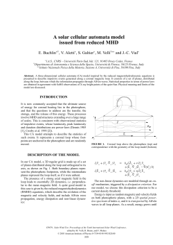
Universit`a degli Studi di Padova AXIAL FLUX DEVICE FOR

Università degli Studi di Padova
DIPARTIMENTO DI INGEGNERIA INDUSTRIALE
Corso di Laurea Magistrale in Ingegneria Elettrica
Tesi di laurea magistrale
AXIAL FLUX DEVICE FOR ELECTROMAGNETIC
CONVERSION/SUSPENSION APPLIED TO A FLYWHEEL SYSTEM
DISPOSITIVO A FLUSSO ASSIALE DI
CONVERSIONE/SOSPENSIONE ELETTROMAGNETICA PER
L’AZIONAMENTO DI UN VOLANO
Candidato:
Relatore:
Franco Bortot
Prof. Andrea Tortella
Matricola 1034176
Correlatore:
Prof. Mauro Andriollo
Anno Accademico 2012-2013
Alla mia famiglia,
per il costante sostegno in questi anni di studio.
Contents
Riassunto Esteso
Introduzione . . . . . . . . . . . . . . . . . . . . . . . . . . . . .
Accumulo cinetico su grande scala . . . . . . . . . . . . . . . .
Macchina sincrona lineare omopolare ed esempio applicativo
Conclusioni . . . . . . . . . . . . . . . . . . . . . . . . . . . . .
.
.
.
.
.
.
.
.
Abstract
1
Introduction
1.1 Overview . . . . . . . . . . . . . . . . . . . . . . . . .
1.2 Grid Services . . . . . . . . . . . . . . . . . . . . . . .
1.3 Hydraulic Storage . . . . . . . . . . . . . . . . . . . .
1.4 Compressed Air Energy Storage (CAES) . . . . . . .
1.5 Uninterruptible Power Supply (UPS) . . . . . . . . .
1.6 Cost Analysis . . . . . . . . . . . . . . . . . . . . . .
1.6.1 Flywheels as suppliers of Regulation Power
1.6.2 NaS Batteries . . . . . . . . . . . . . . . . . .
1.6.3 Generic Comparison . . . . . . . . . . . . . .
i
i
iii
iv
x
1
.
.
.
.
.
.
.
.
.
.
.
.
.
.
.
.
.
.
.
.
.
.
.
.
.
.
.
.
.
.
.
.
.
.
.
.
.
.
.
.
.
.
.
.
.
2
2
4
6
8
10
13
13
17
18
2
Flywheels
21
2.1 Flywheel Technology . . . . . . . . . . . . . . . . . . . . . . . 21
2.2 Materials . . . . . . . . . . . . . . . . . . . . . . . . . . . . . . 24
2.3 Main Installations . . . . . . . . . . . . . . . . . . . . . . . . . 27
3
Large Scale Kinetic Energy Storage (LSKES)
28
3.1 Acting Forces . . . . . . . . . . . . . . . . . . . . . . . . . . . 28
3.2 Energy Density . . . . . . . . . . . . . . . . . . . . . . . . . . 29
4
Transverse Flux Homopolar Synchronous Machine
35
4.1 Overview . . . . . . . . . . . . . . . . . . . . . . . . . . . . . . 35
4.2 Flux Leakage . . . . . . . . . . . . . . . . . . . . . . . . . . . . 36
4.3
5
6
4.2.1 General Geometry . . . . . . . . . . . . . . . . . . . . 36
4.2.2 TFHSM Geometry . . . . . . . . . . . . . . . . . . . . 41
Analytical Design . . . . . . . . . . . . . . . . . . . . . . . . . 46
Design Example
5.1 Overview . . . . . . . . . . . . . . . .
5.2 Materials . . . . . . . . . . . . . . . .
5.2.1 Magnetic Core . . . . . . . . .
5.2.2 Permanent Magnets . . . . .
5.3 Stator Module . . . . . . . . . . . . .
5.3.1 Stator Layout Optimisation .
5.4 Permanent Magnet and Slot Design
.
.
.
.
.
.
.
52
52
56
56
57
60
62
67
FE Analysis Verification
6.1 FEM Exterior Box Influence . . . . . . . . . . . . . . . . . . .
6.2 No-load Results . . . . . . . . . . . . . . . . . . . . . . . . . .
6.2.1 Levitation Force dependence upon Angular Position
6.3 Stability . . . . . . . . . . . . . . . . . . . . . . . . . . . . . . .
6.4 Cogging Torque . . . . . . . . . . . . . . . . . . . . . . . . . .
6.5 Machines Angular Shift . . . . . . . . . . . . . . . . . . . . .
6.6 On-load results . . . . . . . . . . . . . . . . . . . . . . . . . .
6.6.1 Parameters Evaluation . . . . . . . . . . . . . . . . . .
6.6.2 Induced Voltage . . . . . . . . . . . . . . . . . . . . . .
6.6.3 Torque Calculation . . . . . . . . . . . . . . . . . . . .
71
71
74
78
80
83
84
89
89
90
92
.
.
.
.
.
.
.
.
.
.
.
.
.
.
.
.
.
.
.
.
.
.
.
.
.
.
.
.
.
.
.
.
.
.
.
.
.
.
.
.
.
.
.
.
.
.
.
.
.
.
.
.
.
.
.
.
.
.
.
.
.
.
.
.
.
.
.
.
.
.
.
.
.
.
.
.
.
.
.
.
.
.
.
.
.
.
.
.
.
.
.
Conclusions
94
References
96
Riassunto Esteso
Introduzione
Il lavoro di tesi qui svolto verte principalmente sull’accumulo di energia
tramite volani, comprendendo dapprima una descrizione delle tecnologie
presenti ed adottate principalmente per l’accumulo di energia su larga
scala:
• Pompaggio idraulico;
• Stoccaggio di aria compressa (CAES);
• Batterie, fra le più comuni figurano: NaS, piombo acido, Li-ion;
• Volani.
Sebbene esistano molte altre soluzioni tecnologiche, il loro grado di maturità suggerisce di escluderle dal computo, perlomeno nell’ottica di un
orizzonte temporale a breve-medio termine. Fra gli aspetti salienti emerge la difficoltà di comparazione fra le differenti tecnologie, dati i molteplici aspetti da considerare, come per esempio facilità di installazione,
costo di installazione, efficienza nel ciclo carica/scarica, autoconsumi, velocità di risposta del sistema, costo di manutenzione, problemi relativi alla
sicurezza.
I volani impiegati nelle applicazioni di energy storage sono tipicamente
costruiti con fibre di carbonio che, nonostante la loro bassa densità, offrono
resistenze a trazione fino a 2 GPa, quindi permettono alte velocità di rotazione del volano stesso. Essendo la quantità di energia immagazzinata
(tab. I) legata linearmente con il momento d’inerzia e quadraticamente con
la velocità rotazionale del volano, vi è interesse nella ricerca di materiali
resistenti e contemporaneamente pesanti, sebbene ad ora i materiali più
performanti siano le fibre di carbonio (resistenti ma relativamente leggere).
i
Materiale
Acciaio 4340
Materiali compositi
E-glass
S2-glass
Carbon T1000
Carbon AS4C
Densità Resistenza
a trazione
kg
[ m3 ]
[MPa]
7700
1520
2000
1920
1520
1510
100
1470
1950
1650
Massima densità
di energia
[ kWh
]
kg
0.05
Costo
indicativo
e]
[ kg
1
0.014
0.21
0.35
0.30
11.0
24.6
101.8
31.3
Tabella I: Proprietà principali dei materiali impiegati. [17]
La scelta migliore riguardo i materiali può essere operata razionalmente
tramite un’analisi semplificata degli stati di tensione, in cui la densità di
energia per unità di massa è espressa tramite il rapporto fra la resistenza
a trazione e densità del materiale. In fig. I, M1 rappresenta una curva di
indifferenza a densità di energia costante.
Figura I: Scelta dei materiali adatti.
Aumentando l’inclinazione di M1 (maggiore densità di energia) i materiali compositi risultano fra i favoriti, mentre le cermiche sono scartate a
causa della loro fragilità.
ii
Accumulo cinetico su grande scala
L’aspetto principale che limita l’incremento di velocità rotazionale di un volano è rappresentato dal cedimento strutturale causato dagli sforzi centrifughi. All’aumentare della dimensione del volano, gli sforzi tangenziali atti a
compensare l’effetto centrifugo tendono ad avere una componente radiale
che diminuisce all’aumentare del raggio, come spiegato qualitativamente
in fig. II.
Figura II: Distribuzione degli sforzi tangenziali, all’aumentare del raggio.
La diretta conseguenza del fenomeno è che all’aumentare del raggio
(per un determinato materiale), per non incorrere in rotture meccaniche, la
velocità di rotazione deve diminuire. Sommando i due effetti si dimostra
come la densità di energia nel materiale rimanga invariata. Una soluzione
artificiale al problema consiste nell’introduzione di un circuito magnetico
dedicato, atto a compensare la forza centrifuga. La figura III mostra una
possibile configurazione del sistema: un tunnel a forma toroidale, con al
suo interno del materiale rotante disposto in una serie di vagoni interconnessi, tenuto in levitazione e mosso dal circuito magnetico in alto (rosso),
e contenuto radialmente dal circuito magnetico a sinistra (blu). Vi sarebbe inoltre un’importante riduzione nei consumi energetici dati dall’attrito
viscoso qualora venissero adottate tecnologie per fornire un sufficiente
livello di vuoto all’interno del tunnel.
Figura III: Dettagli della soluzione proposta. A sinistra è presente una rappresentazione
dei circuiti magnetici adottati.
iii
In termini di densità energetica, valutazioni numeriche mostrano come
un limite inferiore alla velocità possa essere fissato a 300 m/s, scegliendo
quest’ultima come specifica di progetto. Data la velocità del materiale rotante, è possibile calcolare l’ammontare di pressione magnetica necessaria
al contenimento centrifugo dei vagoni, e rapportarla alla superficie laterale disponibile del tunnel. Da ciò è possibile ottenere il valore d’induzione
magnetica necessaria allo scopo e confrontarlo con valori normalmente
presenti nelle macchine elettriche (0.5 - 1 T). A titolo esemplificativo, un
esempio di progetto dove l’induzione magnetica è stata fissata ad 1 T
e la velocità tangenziale a 300 m/s ha portato alle dimensioni del toro:
R = 3km, Φ = 2m, assumendo come materiale rotante acciaio con densità
di 7800 kg/m3 . In termini di costo specifico, il risultato più significativo è
rappresentato dal costo per unità di energia immagazzinata, riguardo al
solo materiale rotante. Infatti assumendo un costo specifico di 0.5 e/kg per
l’acciaio, si ottengono 40 e/kWh. Il risultato appare interessante, perlomeno
al livello di analisi adottato, in quanto in un’ottica di comparazione dei costi rispetto ad altre tecnologie permette un ampio margine economico per
la costruzione di tutte le infrastrutture necessarie alla levitazione, il tunnel
e i dispositivi per creare il vuoto. Come indice di confronto, le batterie
piombo-acido hanno un costo per unità di energia stimabile in 120 e/kWh.
Alla luce dei potenziali benefici economici, rimangono tuttavia irrisolte
una serie di sfide tecnologiche necessarie ad assicurare il corretto funzionamento della struttura, in primis la gestione attiva del traferro necessaria
a provvedere la stabilità del materiale rotante ad una velocità cosı́ alta.
Macchina sincrona lineare omopolare ed esempio
applicativo
Per l’azionamento di un volano è stata scelta una macchina sincrona lineare
omopolare, con flusso trasverso prodotto da un magnete permanente. La
geometria (fig. IV) permette di assolvere contestualmente due funzioni:
• Sospensione magnetica del volano, grazie alla forza attrattiva fra
statore e rotore esercitata dal magnete permanente;
• Propulsione del rotore, grazie all’iniezione di un’opportuna terna di
correnti trifase nell’avvolgimento di statore.
iv
Figura IV: Geometria della macchina sincrona lineare omopolare, a flusso trasverso.
I vantaggi di tale configurazione possono essere riassunti in:
• Basse perdite rotoriche, dovute anche all’assenza di circuiti sul rotore
stesso;
• Alto rendimento, tipico delle macchine sincrone;
• Modularità della geometria;
• Unica parte rotante composta da blocchetti di materiale ferromagnetico.
D’altro canto le macchine lineari soffrono di effetti di bordo, la configurazione omopolare prevede anche un basso sfruttamento del rame di statore, quindi un fattore di potenza ridotto. A causa dell’alta riluttanza del
magnete i flussi di dispersione hanno un contributo non trascurabile, di
conseguenza vari metodi sono stati adottati per contabilizzarne l’effetto.
Data la tridimensionalità intrinseca della macchina, in sede di progetto si
sono introdotte due sezioni bidimensionali semplificate implementate tramite codice agli elementi finiti. Esse hanno potuto fornire un’indicazione
attendibile dell’importanza dei flussi di dispersione, in particolare riguardo alla porzione di flusso prodotto dal magnete che raggiunge il traferro.
Sono quindi state implementate numerose simulazioni bidimensionali, al
variare di coefficienti adimensionali rappresentativi della geometria, per
v
poi condensare i risultati tramite delle funzioni interpolanti. Nell’ottica di
proporre una soluzione integrabile con prodotti esistenti, si è scelto di progettare un azionamento alternativo a quello attualmente implementato nei
volani prodotti da Beacon Power di 4a generazione. Tale sistema utilizza
una macchina sincrona a flusso radiale, a magneti permanenti, in combinazione con cuscinetti magnetici ibridi (in parte costituiti da magneti, in
parte da avvolgimenti controllati attivamente). Il tutto è mantenuto sotto
condizioni di vuoto per ridurre le perdite enegetiche prodotte dall’attrito
viscoso.
La soluzione proposta (fig. V) consta invece di tre macchine principali, ognuna delle quali contenente una serie di macchine lineari sincrone
omopolari, disposte su di una circonferenza. La parte ottagonale rossa
rappresenta l’insieme degli statori, mentre i blocchetti magnetici di rotore
sono calettati su di un’unica flangia e solidali col volano.
Figura V: Geometria dell’azionamento proposto.
Date le alte velocità di rotazione, per il circuito magnetico si è scelto
un materiale in polvere (Soft Magnetic Composite), a cui viene impressa la
geometria voluta tramite operazioni di stampaggio e riscaldo. Fra le varie
caratteristiche, rispetto ai lamierini, tali materiali permettono di contenere
le perdite per isteresi e correnti parassite generate dalle alte frequenze
delle grandezze in gioco. Un riassunto delle specifiche adottate per il
progetto della macchina è contenuto in tab. II, dove si è assunto un ciclo
di carica/scarica di 6 ore come riferimento.
vi
Grandezza
Valore
Forza di levitazione richiesta
10
Velocità di rotazione minima
8000
Velocità di rotazione massima
16000
Numero di macchine
3
Numero di statori per macchina
8
Potenza richiesta
4.17
Energia immagazzinata
25
Coppia in caso di velocità minima
5
Unità di misura
kN
rpm
rpm
kW
kWh
Nm
Tabella II: Specifiche della macchina elettrica.
Essendo presenti vari gradi di libertà nella scelta della geometria di statore, si è adottato un approccio di ottimizzazione multi obbiettivo che ha
permesso di massimizzare l’area dei poli e contemporaneamente ridurre gli
effetti di curvatura inevitabili dalla disposizione circonferenziale delle macchine. In fig. VI è rappresentato il risultato successivo all’ottimizzazione,
una volta scelto il numero di statori per macchina p=8.
Figura VI: Vista dall’alto della disposizione statorica ottimizzata, nel caso di otto statori.
Come si può notare vi sono dei tratti angolari in cui un rotore, nel
passare da uno statore al successivo, incontra una bassa superifcie di accoppiamento con lo statore, portando ad un decremento delle performance
medie. È stato quindi introdotto un coefficiente maggiorativo delle prestazioni basato sull’area media di accoppiamento fra statore e rotore (fig.
VII).
I risultati dei principali studi parametrici sono riassunti nelle figure
VIII - XI, dove si può notare un comportamento stabile della macchina
vii
Figura VII: Vista dall’alto del’area di accoppiamento, per differenti posizioni rotoriche.
per quanto riguarda sbilanciamenti lungo il piano ortogonale all’asse di
rotazione (piano xy), mentre un controllo attivo del traferro è richiesto
lungo l’asse verticale (asse z).
Figura VIII: Forza di levitazione al variare dell’angolo rotorico.
viii
Figura IX: Forza di levitazione al variare del traferro.
Figura X: Forza stabilizzante lungo x, in caso di decentratura. I valori si riferiscono ad
un insieme di 8 statori e rotori.
Figura XI: Coppia di impuntamento, al variare della posizione rotorica.
ix
Riguardo ad un singolo rotore, i principali risultati numerici e una
comparazione fra il metodo analitico adottato e il modello FEM 3D sono
riassunti in tabella:
Grandezza
Metodo analitico Metodo FEM 3D Unità di misura
Forza di levitazione media
417
380
N
Coppia media
0.208
0.187
Nm
Flusso del magnete
1.73
1.65
mWb
Flusso al traferro
1.02
0.996
mWb
Tabella III: Comparazione fra i risultati dei due metodi considerati.
Come si può notare vi è in generale una tendenza del metodo analitico a fornire soluzioni che sovrastimano le performance, rispetto a quanto
valutato più accuratamente tramite FEM. Va tuttavia specificato che il basso costo computazionale del metodo analitico lo rende preferibile in prima analisi, per poi correggere eventuali deviazioni rispetto alle specifiche
tramite modifiche alla geometria e validazioni FEM.
Conclusioni
La macchina elettrica proposta è stata dimensionata e validata, riscontrando differenze fra stime analitiche e valutazioni FEM con errori contenuti
all’interno del 15% per la maggior parte delle grandezze considerate. Il
metodo proposto che comprende la valutazione di analisi FEM 2D semplificate ha mostrato la maggior congruenza con i risultati, rispetto ad
altre metodologie esaminate (reti magnetiche). Le problematiche su cui
focalizzare futuri studi comprendono la riduzione della coppia di cogging,
la valutazione delle perdite per correnti parassite e isteresi magnetica,
nonchè un’analisi più approfondita dell’utilizzo del materiale magnetico,
che può portare ad una geometria ad angoli smussati senza pregiudicarne
le caratteristiche di permeabilità.
x
Abstract
In this work of thesis multiple aspect of energy storage technologies are
discussed, focusing on kinetic energy storage by mean of flywheels. The
first two chapters comprise a literature review, outlining state of the art
technologies together with their major characteristics concerning costs,
ease of siting, safety, efficiency, speed of response and maintenance issues.
The third chapter undertakes a feasibility analysis of a large scale kinetic
energy storage (LSKES), showing cost advantages that may arise from an
increased dimension of the system, together with technological challenges
to be faced.
Finally, last chapters present a novel application of a transverse flux
homopolar synchronous machine (TFHSM) on a flywheel energy storage
system (FESS). Some of the characteristics of TFHSMs are well suited to
the specifications required by an electric machine interfacing FESSs to the
power grid. In particular, two functions may be embedded:
• accelerating/decelerating torque;
• upward levitation force, that would enable the flywheel to be completely magnetically suspended without the need of additional magnetic or mechanical bearings.
TFHSMs are already commercially employed, mainly in the case of low
maintenance industrial movers or electric powered public transport. On
the other hand flywheels are a proven technology that has been mainly
used in the past for motion smoothing by mean of their inertia. However
nowadays, thanks to the composite materials performance achievements,
new applications in energy storage are becoming attractive. Despite their
low density composite materials can bear mechanical stresses of approximately an order of magnitude higher than conventional metals, resulting
in a theoretical stored energy density that is competitive with modern
batteries.
1
Chapter 1
Introduction
1.1
Overview
In the past decade the interest for CO2 emissions reduction and environmental issues in general had grown in importance, creating the spark that
allowed renewable energy sources to enter the scene of global energy production. Concentrating on the electricity production, the only form of
renewable energy that has been exploited on a large scale for many years
is the hydroelectric one. Most of such power plants are composed by a
dam that allows energy storage and thus power delivery regulation.
By way of contrast, emerging technologies such as wind turbines and
photovoltaic are inherently intermittent and only partially predictable [1,
2, 3, 4]. As a consequence, if we assume an increase in power production
over the years to come by intermittent renewable energy sources (IRESs),
the grid stability will become of concern [5, 6].
There are basically two ways of facing the spread between the demanded and the produced power:
• Power modulation of both conventional power plants and renewable
energy sources allowing for regulated generation;
• Energy storage, near the IRESs plants and close to the main centres
of consumption as well.
The former solution is the simplest to implement, at least while adequate
energy storage facilities aren’t available. However, it raises operating
issues for conventional plants, mainly due to the fact that they’ve been
designed and built assuming a constant power output. As power output
changes significantly and quickly, steam cycle components such as heat
exchangers are thermally overstressed with respect to their rated operation.
2
An estimate of the life-expectancy reduction of power plants that could
be caused by these stresses has been made by [7], even though it is clear that
this is an important risk conventional power plants operators are implicitly
bearing due to the energy free market and growing shares of IRESs. This,
together with the efficiency reduction that occurs for power outputs lower
than the nominal rating, opens new possibilities for energy storage on a
large scale.
At the moment, the latter solution is worldwide led by hydraulic storage [8], that accounts for more than 100 GW of installed power and more
than 99% of the market [9]. However some intrinsic aspects of the technology may be of limitation for certain purposes. For example, it cannot
be installed on flat zones, where cities that need energy storage can be
located. Wide extension power lines from mountains to cities can mitigate
the problem, but only partially as they introduce losses, stability margin
reduction and construction disapproval from interested population. Another limitation is the delivery of high power ancillary services, if required
in locations where hydraulic storage is not feasible. Concerning this aspect, fig. 1 shows that not all the kinds of power plants are suitable for grid
services requiring high speed of response, and even though hydro power
plants have quicker response than other thermal ones, they still result to be
excessively slow for some specific purposes. On a grid perspective, it must
Figure 1: Comparison of the adjustable load rates of four power plants. [8]
be pointed out that according to Mazzocchi et al. [10], small dimension distributed electrical generators tend to lack in provision of spinning reserve,
and this can be compensated only through appropriately programmed
inverters connected to energy storage devices.
3
1.2
Grid Services
Energy storage has multiple functions that can be classified by mean of the
average time involved in the function delivery. An overall representation
Figure 2: Classification of main applications of energy storage on a time basis. [10]
of the services that are required for a proper and optimized working grid
are expressed by fig. 2, including services that are likely to be heavily
augmented in the years to come, as the ones laying on the right side of the
scheme. More precisely, a detailed description of each function comprises:
• Time Shift - Use of systems in order to delay the electric energy
consumption. Its typical time span is 1 to 10 hours. It must be
pointed out that thanks to the price difference of electricity from
day to night, energy storage devices that can perform time shift
may become attractive on a trading perspective (so called Energy
Time Shift). This has the advantage of lowering peak prices that
occurs whenever the demand is critical with respect to the supply.
Another point of view may be the TSO’s one, who may be interested
in avoiding the construction of new lines or potentiation of existing
ones, as one demand zone becomes critical in only some periods of
the whole day. It is commonly defined as Investment Deferral;
• Power Balancing - Use of energy storage with the goal to face both
the demand curve (which has generally low price elasticity, thus on
4
the TSO perspective it is non-modifiable and unknown a priori), and
the aleatory production curve of IRESs. Sub-applications as Load
Following allows a better use of conventional power plants, as the
spread between demand curve and IRESs production curve becomes
more predictable;
• High Power Ancillary Services - It generally requires a response time
lower than a second, which is crucial for short term grid stability.
Ancillary services are a wide family of grid capabilities that are in
charge of managing grid mismatch. For example, Spinning Reserve
is usually delivered by the power plant generators, with the goal of
keeping stable values of frequency as soon as a power interruption
occurs. Batteries and other devices connected to the grid through
an inverter can help performing the task, with the advantageous
possibility of installation directly on the critical zone. On the other
side, Power Quality is gaining importance also due to the raising
content of current harmonics generated by electronic devices.
The power regulations that every time are carried out in the grid, in order
to constantly match demand and supply (including transmission losses),
are divided into three sets. The reason behind the classification is related to
the technology and infrastructure that performs it. For short term fluctua-
Figure 3: Components of a load curve. [8]
tions (up to some minutes), an automatic system also referred as primary
regulation changes the power output in order to follow the request, but a
variation in frequency occurs. For long term fluctuations (up to 30 minutes), secondary regulation has the duty to reset the grid frequency to the
nominal value. Finally, the daily load curve is followed at most by mean
5
of an energy market called day-ahead market, where the demand for the
day to come is forecasted together with IRESs contributions, and the energy supply is contracted among producers, big private consumers and
publicly owned companies that aggregate small consumers. The traded
energy contract has usually minimal duration of 1 hour.
1.3
Hydraulic Storage
Hydropower is one of the oldest ways to produce electricity, dating the
first large scale applications at the end of 19th century. It can be seen in fig.
Figure 4: Global electricity generation by fuel, 1973-2010. [11]
4 that hydropower historically kept a slightly shrinking production share,
with installations that grew less than proportionally to demand. Nevertheless, it still contributes to approx. 17% of global electricity production.
However only a fraction of the total installed plants is capable of pumping, mainly because it requires additional investments or site features like
a lower reservoir, ternary groups or reversible Francis turbines and electric
equipment that performs variable speed operation. Despite its leader position in energy storage, it has some disadvantages that had limited new
installations over the last decades, as seen in fig. 5, namely because of:
• Environmental impact of reservoirs - Concerns about phenomena
as fragmentation of river ecosystems, reservoir sedimentation, river
road and coastal erosion, changes in water temperature and oxygenation;
6
Figure 5: Pumped hydro trends. [8]
• Risk - Events in the past have already shown that disasters due to
dam breakdown or landslide caused by geological instability and
consequential overflow are possible. Because of this and the former
point, social acceptance becomes crucial in successful projects, as in
most large scale engineering constructions;
• Suitable locations - By the fact that installations increased in absolute
terms, it is more difficult to find sites (technically referred as siting)
that meet the requirements: geological stability, head (difference in
water elevation between upper and lower reservoirs) and others of
minor importance.
All the points are binding in different ways among various countries and
continents, depending upon the amount already deployed of hydroelectric
potential.
Costs are expected to be constant in the future, as the technology is
completely mature: according to [8], a new installation would cost 2100
- 2600 e/kW, sub divided into dam (30%), channel (21%), generator (15%),
civil engineering (9%) and balance of plant (25%).
Seawater applications may be an interesting solution where sufficiently
steep shores are present [10], since they enable the construction of a single
upper reservoir, exploiting the sea as lower reservoir. The 30 MW Yanbaru
project in Okinawa (Japan) has been the first concept demonstration. Sea
corrosion and its mitigation is estimated to raise plant costs of 15% [8] with
respect of a benchmark freshwater plant.
7
1.4
Compressed Air Energy Storage (CAES)
Based on a reservoir of compressed air, CAES systems allow to store energy
through compression and consequential (time deferred) expansion of air.
There are mainly two classes of plants, fired CAES and unfired CAES.
The distinction is due to the fact that during the compression phase, air
increases its temperature, whereas during the expansion phase it tends to
cool down, arising the problem of ice creation in the turbine. In order
to cope with these aspects, heat can be stored during compression and
then be given back to the air during expansion (diabatic CAES) or external
heat may be provided by combustion of a fossil fuel, generally natural gas
(diabatic, or fired, CAES). Most important layouts can be seen in fig. 6,
where both diabatic and adiabatic configurations are featured.
Figure 6: Different plant layouts. [8]
The most important installations are diabatic CAESs located in USA
(McIntosh, Alabama, 110 MW) and Germany (Huntorf, 290 MW), both
have been built decades ago (1991 and 1978 respectively) and rely on a
cavern, operating at pressures in the range of 45 - 75 bar. Despite the low
number of plants existing, reliability on the long term has been proved
thanks to this two proof of concept sites [9].
A further distinction between aboveground and underground CAES
refers to the way as air is stored. Underground CAES is the only one
8
that has been built on a large scale, up to now; aquifers and caverns are
the preferred sites. Aboveground CAES attempts to free this technology
from the adequate location constrain, opting for tanks (possibly supplied
from other industries that have already reached maturity stage, such as
Oil & Gas or technical gases). As a result, they can be installed wherever
the grid requires energy storage, and generally permit also lower nominal
power ratings (some MWs). Conversely, underground CAES shows cost
advantages due to the tank avoidance.
Probably the most important drawback lays in the low efficiency, attaining an electrial efficiency (expressed as electric energy delivered over
electric energy consumed) of 65% in case of adiabatic CAES and 75% in
case of diabatic CAES coupled with CCGT. In terms of primary energy
efficiency (electric energy delivered over total thermal energy consumed),
adiabatic CAES reach up to 27% and diabatic CAES, in the best foreseeable
layout as integrated with fossil fuel plants, 38% [9].
In the case of adiabatic CAES, the thermal energy storage becomes
an issue, with various technologies available to meet this need. Mainly
coming from the Concentrated Solar Power (CSP) sector, solutions range
across water (up to 100°C, at ambient pressure), molten salts (150 - 550°C),
diathermic oil (up to 400°C), blocks of concrete (up to 400°C).
Concerning costs, in case of diabatic CAES, a part of the variable cost
component is directly linked with fuel price (generally natural gas), hence
hardly predictable in the future. For an underground diabatic CAES,
plant costs are estimated to be 1000 - 1250 e/kW, as far as 2200 e/kW for an
abovegound adiabatic CAES. Life expectancy is projected to be comparable
with pumped hydro plants (35 years), or in terms of operative cycles,
higher than 13000 cycles. Already existing installations have empirically
demonstrated the long-lasting performances of the technology.
9
1.5
Uninterruptible Power Supply (UPS)
Critical applications of electric energy such as data centres, banks and
medical equipment require a continuous power delivery, despite a failure
of the main grid. Moreover, sensible devices as the electronic ones must
be fed with relatively high quality of power, i.e. a three phase voltage
waveform close to the ideal isofrequency, iso-amplitude sinusoidal one.
Figure 7 shows different sensibilities of electric devices to voltage drops.
Proper functioning of the appliances is reached through an approach
that takes into account both devices sensibility and grid disturbances,
because their combination allows an estimate of the yearly outages in the
requested service. As it can be seen in fig. 8, most of the grid anomalies
Figure 7: Electric devices affected areas by the momentary voltage drop. [12]
are concentrated in a range of few seconds, even if occasional long lasting
interruptions would require a wider energy backup. Given the two charts
it can be outlined the frequency of outages due to voltage drops, for a
particular application: for example, if computers only must be fed by UPS,
probably there is no such need to provide extremely quick response, at
least with respect to others more sensible devices.
Power conditioning is a concept that is related to UPSs as most of the
requirements by Power Quality can be delivered by a unique integrated
system. An ideal UPS must face all the following issues at the same time:
10
Figure 8: Statistics of anomalies on European MV grid. Source: UNIPEDE DISDI.
• Harmonics;
• Voltage spikes or sustained overvoltages;
• Voltage drops;
• Interruptions;
• Flicker;
• Imbalance between phases.
Manufacturers generally provide solutions that address many of the aforementioned points. The two major technologies used nowadays in the UPS
field are batteries and flywheels (often referred as rotary UPSs). In addition,
a distinction between online, line-interactive and stand-by configurations
shall be made.
Stand-by layout is composed by a 2-ways switch that is, in normal
operation mode, turned to feed the load through the mains. As soon as a
fault is detected, the switch changes state and feeds the load through UPS.
Switching time is generally contained under 25 ms.
11
On the other hand, line-interactive configuration adds an autotransformer between the grid and the switch, which allows to cope with continuous overvoltages or undervoltages, acting on the on load tap changer,
instead of relying on the UPS.
Finally, online UPS allows a complete decoupling between grid and
appliances. It is designed for being constantly in operation, converting
the power from the grid to a DC bus (where the batteries or flywheel are
connected) and then feeding the loads through an inverter. This is why
it is also called double-conversion UPS. As a consequence, in case of an
outage there is virtually no effect over the appliances, at the expenses of
an increased initial investment (due to the higher number of components
and their size, this kind of UPS is generally more expensive).
Concerning the two main energy storage technologies used in the UPS
field, some characteristics of flywheels may result advantageous with respect to batteries, as well as others are penalizing. According to [34], pros
of flywheels can be summarized as follows:
• No need of air conditioning in the energy storage room, nor temperature monitoring;
• No appreciable performance degradation over time;
• Expected life far higher;
• MTBF (Mean Time Between Failure) from 6 to 10 times higher;
• Higher crest factor (ratio between peak value over RMS value of
current);
• High short circuit current, that enables sure intervention of protection devices (valid only for flywheels directly connected to the grid
through an electrical machine);
• No influence of operating temperature over usable energy;
• Precision in the compute of available energy. When dealing with batteries, this estimate may be tricky and affected by many parameters.
Instead, drawbacks are:
• Need of diesel generator backup in order to face long lasting outages;
• Higher stand-by consumption;
• Noise and vibrations;
• Convenient only for high powers ratings.
12
1.6
Cost Analysis
This section aims to offer detailed cost comparison, even though a wide
variety of factors is needed to be specified for each technology. Among
all the energy storage solutions, flywheels and NaS batteries are examined
more deeply than the others.
1.6.1
Flywheels as suppliers of Regulation Power
In order to evaluate costs and compare various technologies, some assumptions should be made. Since it is calculated the economic effort
needed to provide a certain regulation power, a fixed amount of it has
been chosen, comparing the NPV (Net Present Value) of the considered
solutions [13]. By definition, the NPV consists of the sum of discounted
cash flows involved in an investment: in this case it will account for plant
costs, O&M costs (discounted at an appropriate discount rate, in order to
obtain values that are present, instead of projected into the future) and any
further cost related to the flywheel operation. Generally speaking, benefits
of energy storage for regulation purposes can be summarised as follows,
independently from the technology used to provide it:
• Increase in peak and base load capability of the grid - Assuming
for simplicity a small grid consisting of a power plant, a line and a
consumption centre, if energy storage is installed close to the latter
there would be the possibility to use the line at a higher power rating
all the time, as peaks are dispatched by the energy storage device;
• Reduction of losses, as regulation power contributes to power lines
losses. This can be seen more clearly in the example figure 9, where a
long term current component is shown, together with a summed zeromean random signal to represent regulation current in the power line.
By the fact that usually power lines operate at almost fixed voltage,
a ripple in current means an equal ripple in power, given a constant
power factor. In addition, the mean of the two waves is the same,
thus overall the same amount of energy is dispatched. By squaring
the RMS values of the two curves and integrating, a 3.6% higher
figure is obtained in the case of long term + regulation component;
• Reduced power line congestions, as a consequence of the former
points;
• V-Q control, thanks to the inverter capabilities (if the energy storage
technology calls for it);
13
• Contribution to ’Black Start’ of conventional plants. In case of a
blackout, thermoelectric plants need external power to supply their
auxiliary systems in the goal of bringing the grid back on-line, thus
under this circumstances flywheel energy storage can effectively help
the conventional plants to restart.
Figure 9: Long term component and regulation component.
A main distinction between energy applications and power applications is important, mainly because some technologies may result favorable
for one use but too expensive for another one. For this purpose, [10] shows
the suggestive table 1 describing the suitability of many technologies, depending over the grid service expected time duration. As flywheels appear
to be conveniently viable only for short term applications (high power),
this purposes are considered in the following treatise. Regulation life cycle
costs have been calculated by [13], comprising the main alternative technologies. A particularity of this study is the inclusion of fossil fuel plants
(that do not perform energy storage): it makes sense by the fact that under
some assumptions such technologies may result with comparable costs
with respect to storage. This is an important aspect of the overall energy
storage issue: on a merely cost point of view, sometimes it is cheaper to
produce the peak power through peaker plants (that generally have low
initial plant costs but high operation and maintenance costs) than exploiting the reserve provided by energy storage. This condition only holds in
particular cases, e.g. if the storage technology has particularly high costs
and no CO2 tax is charged, like today in the USA.Considering only a subset
of the technologies mentioned before, under the hypotheses listed in tables
2 and 3, the study results are presented.
14
Technology
Hydraulic
CAES
Sodium-Sulfur
batteries
Sodium-Nickel chloride
batteries
Li-ion batteries
Ni-Cd batteries
Ni-MH batteries
Pb acid batteries
Flow batteries
Flywheels
SMESs
Supercapacitors
Time Shift Power Balancing Power Ancillary
Services
X
?
X
X
?
X
X
X
?
X
X
?
X
X
X
X
X
X
X
X
X
X
X
X
X
?
X
X
X
X
?
?
?
X
X
X
Table 1: Energy storage technologies and their best use. X represents unsuitability,
Xrepresents suitability, ? represents uncertainty. [10]
In addition, it has been hypothesized a complete substitution of the
lead acid batteries every 7 years. No forecast over electric energy and fuel
price trend nor increase in maintenance costs has been made, assuming
as valid the figures evaluated for the first year of study. Concerning the
batteries, a roundtrip efficiency of 90.25% (95% per semi-cycle) has been assumed, together with a 20% DOD (Depth Of Discharge) nominal cycle. An
advantage that could lower the cost related to inverter-based technologies
is represented by their fast response time. More specifically, the authors of
[13] outline how often happens that the traditional regulation (performed
through power plants electric generators) shows to be excessively slow,
resulting in regulation power that is against the current demand. For example, an injection of power even though the demand increased some
minutes ago, but now has shrank. As a consequence, they introduce an
X factor in order to account for the upgraded capabilities that flywheels
and batteries would lead. Even if it has still to be deeply investigated, a
estimate is X = 2, i.e. at installed power parity, inverted-based technologies
deliver twice the service.
15
Item
Regulation power
Number of cycles per year
Evaluation time frame
Yearly Maintenance
Expression/Value
20 MW
8760
30 years
Lead acid: 2% of installation cost
Flywheels: 11.6 USD/kW + 1.2 MWh/(MW*day) of losses
Fossil fuel plants: +0.5% of regular maintenance
Increased fuel consumption
Fossil fuel plants only:
allocated to regulation
2.7% - 3.7%
CO2 tax
17 USD/ton
Table 2: Main assumptions included in [13]. First part.
Figure 10: NPV hourly cost comparison. [13]
Figure 11: NPV hourly cost comparison including CO2 and an X factor equal to 2. [13]
16
Item
Discount rate on cash flow
Electricity cost, station power
Electricity cost, transaction power
Regulation revenue
Rating for base fossil plants
Rating for peaker fossil plants
Plant Cost
Availability reduction
due to regulation
Expression/Value
7.5%
50 USD/MWh
70 USD/MWh
52.5 USD/MW per service hour
400 MW
75 MW
Lead acid: 150 USD/kWh +
165 USD/kW of power electronics
Flywheels 1630 USD/kW
Coal base load: 2000 USD/kW
Coal peaker: 1000 USD/kW
Gas base load: 600 USD/kW
Gas peaker: 800 USD/kW
Fossil fuel plants only: 6%
Table 3: Main assumptions included in [13]. Second part.
Both the charts outline important cost indexes, together with description of contribution to overall cost by maintenance, equipment, energy
and CO2 , where considered. Flywheels appear to be convenient in the
long term, mainly due to the low duration of lead acid batteries and the
high initial cost of flywheels. In the case of this study, fossil fuel plants
have proven to be not economically advantageous, in particular if the X
factor is considered and a carbon tax is foreseen in the years to come. In
addition, a strong hypothesis over the yearly amount of cycles (one cycle
per hour, 24 hours a day, 7 days a week) is one of the factor that helps the
most to show flywheels advantages.
1.6.2
NaS Batteries
A technology that is currently becoming attractive on a point of view of
grid energy storage is represented by Sodium Sulfur (NaS) batteries. Even
if their general application has a wider time horizon than high power ancillary services, they have good overload capabilities (up to 6x the continuous
rating), fast response and forecasts of substantial cost reduction in the future. According to [36], their cost is 350 USD/kWh and 2000 USD/kW. On an
energy density perspective, they can achieve 150 - 240 Wh/kg and 150 - 230
W/kg of power density and perform up to 5000 cycles (at DOD < 100%).
17
Some security concerns arose after the 2011 fire incident in Tsukuba.
Indeed, one of the major drawbacks consists in the high operating temperature (300°C - 350°C), that is necessary in order to keep the elements
liquid. As a result, proper thermal insulation is required, but generally no
additional heating system is required, once the battery is running, thanks
to the heat generated by the charge-discharge process itself. Fire hazard
is related to the molten sodium that spontaneously burn if in contact with
air or humidity.
1.6.3
Generic Comparison
This part has the goal of a comprehensive, even if not deeply detailed
description of the main aspects of the energy storage technology. Moreover,
often figures are displayed only in form of tables or inserted in text, thus
limiting a comparison among all the aspects. It should be clear that up
to now there is no clear winner in this market, some technologies may
perform better than others only in specific tasks, and research (and the
pace it will take) will eventually show the best options.
In the following charts the author took data from the cited literature,
performed an empirical mean operation (where data were homogeneous)
and integrated with subjective impressions if figures were missing. Even
though a range of values associated to each parameter would be more
descriptive, often it is hard to aggregate data from different studies, as
they comply with different assumptions. Furthermore, a single number is
easier to represent and gives a more immediate feeling of the proportions
when performing visual comparisons.
Underground Diabatic CAES
Pumped Hydro
Flywheels
NaS Batteries
Li-Ion Batteries
Lead-Acid Batteries
e/kW
e/kWh
1250
2100
1254
1538
410
143
156
263
5015
269
650
100
Ease of siting Time response Stand-by losses / Efficiency N. of cycles
self-discharge
10 = 100%
5
4
1
6.5
20000
2
4
1
7.5
20000
8
9
10
9.2
20000
7
9
5
9
3500
10
9
5
9
4000
10
9
6
8
1000
Table 4: Study assumptions
The radar plot depicted in fig. 12 is obtained scaling all the values
contained in table 4 on a range of 0 to 10. In other words, the worst
performing technology, for a specific index, has assigned value of zero. In
this sense, it may be referred as relative.
Some other aspects may be better seen through a scaling on absolute
values, as in fig. 13. For example, efficiency ranges from 65% to 92%,
18
and the first graph implicitly hides this aspect. Caution should be used
while considering some axes (the stand-by losses axis, for example), as they
are directed conversely than others: the lower, the better. Some sharp
Figure 12: Radar plot in relative terms.
differences among the considered technologies are worth to be pointed out:
Flywheels have an energy specific cost that is an order of magnitude higher
than other technologies. As a consequence, only high power, low energy
applications or duties where it is required a lot of cycles per year and fast
response simultaneously can be envisaged as convenient for flywheels.
CAES shows low energy density cost, as well as long lasting availability,
but is penalized in efficiency and siting, together with slow response with
respect to technologies that use inverters.
Overall, it’s not easily understandable where the best performing solution lays, whereas single applications can be considered with the goal to
rank a preferred technology for each of them.
A Levelized Energy Cost (LEC) approach can help reducing the number of variables to consider, but still requires assumptions concerning the
evaluation time frame, required return on investment, discount rate and
more specific hypotheses for each technology, resulting in a partial view
of the big picture.
19
Figure 13: Radar plot in absoulte terms.
20
Chapter 2
Flywheels
2.1
Flywheel Technology
The theory behind flywheels is well known and consolidated and no quantum leap improvement is expected in the near future. Rather material
advance (together with the progress in power electronics) is the factor that
allowed the development of commercial flywheels with a focus on energy
storage, instead of mechanical load smoothing as it used to be until some
decades ago.
The operational principle can be explained recalling the theory used
for thick walled pressure vessels [14], i.e. the study of a solid body under
axisymmetrical geometry and stress conditions. The stresses are calculated
through:
Figure 14: System of cylindrical coordinates, located on a general point out of the rotation
axis.

B
ν
2


σr (ρ) = A − ρ2 − Cρ + 1−ν σl


ν
σt (ρ) = A + ρB2 − Dρ2 + 1−ν
σl
where
C=
3+ν
σ0
8
D=
1 + 3ν
σ0
8
21
σ0 = ρmat ω2 r2ext
(2.1)
(2.2)
Symbol
Expression - value Unit of measure
Comments
2
N
σr
Radial stress
/mm
2
N
/mm
Hoop stress
σt
ν
0.3
Poisson’s coefficient
r
ρ
Adimensional radius
rext
A, B, C, D
Constants to be calculated
N/mm2
σl
0
Longitudinal stress
3
kg
/m
ρmat
Material density
rad/s
Angular velocity
ω
Table 5: Symbol definition
Notice that σl is null only for the particular case of flywheels, as it
accounts for possible forces that would act on the axis direction.
Considering a yield criterion, the Von Mises equivalent tensile stress is
calculated through:
q
σVM = σ21 + σ22 + σ23 − (σ1 σ2 + σ2 σ3 + σ1 σ3 )
(2.3)
where subscripts 1, 2 and 3 are representing the three main stresses directions. In our specific instance, they coincide with r, t, l unit vectors defined
in fig. 14.
Figure 15: Stresses along the adimensional radius for a spinning flywheel
In turn, once the system of equations is solved through the imposition
of 2.2 on 2.1 and additional conditions concerning the inner and outer
22
surface, typical behaviors of σr and σt , together with the Von Mises stress
are shown in fig. 15.
The Guest stress in our specific case is coincident with σt , because the
lowest principal component is always equal to zero.
Even if counterintuitive, the flywheel part that is more likely to break
is the interior surface. This is confirmed by both yield criterions adopted.
The approach is valid only for solid bodies, whereas composite material
flywheels are made by a sequence of wound carbon sheets. In order to
use the aforementioned method, it must be verified that the solid hypothesis still holds, together with a control of the differences that anisotropic
behavior of composites may introduce.
In order to gain higher predictive power, viscoelastic and creep models
need to be implemented [15], but a proper investigation of the phenomena
is beyond the content of this thesis.
Fatigue must be explored in depth as well since the typical expected life
of FESSs is 20 years, resulting in tens of thousands of cycles, hence exactly
where the yield strength is subject to degradation:
Figure 16: Generalized speed versus cycles curve indicating the onset of fatigue initiation
cracks at the inner radius of the composite core. [15]
Fig. 16 represents the stress that leads to failure in the inner diameter
(ID), as a function of the number of fatigue cycles applied and the flywheel
mean radius. More precisely, the maximum rotating speed is calculated,
23
which corresponds to a stress that would lead to flywheel failure.
2.2
Materials
As mentioned before, modern flywheels are made by composite materials.
Despite their low density, carbon fibers can yield extraordinary loads over
a direction. Many authors outlined theoretical energy densities for composites, with a precautionary approach it is reported the one proposed by
[16], even if others show higher figures [17]. Neglecting for a moment the
weight of motor/generator, shaft, bearings and housing, such densities are
advantageous with respect of common batteries Li-ion (110-160 Wh/kg),
Ni-MH (60-120 Wh/kg), Pb (30-50 Wh/kg) [18].
Material
4340 Steel
Composites
E-glass
S2-glass
Carbon T1000
Carbon AS4C
Density Tensile strength Max energy density
kg
[ m3 ]
[MPa]
[ kWh
]
kg
7700
1520
0.05
2000
1920
1520
1510
100
1470
1950
1650
0.014
0.21
0.35
0.30
Cost
e]
[ kg
1
11.0
24.6
101.8
31.3
Table 6: Material properties of composites. [17]
The theoretical reason behind composites choice can be explained in a
few equations: assuming as a reference figure 17,
Figure 17: Flywheel schematic drawing.
24
the amount of energy stored in a spinning body is
E=
1 2
Jω
2
(2.4)
where J is the moment of inertia and ω is the angular speed. In case of a
disk, J is given by
π
J = ρmat R4 tω2
4
and in turn the flywheel mass results
m = πρmat R2 t
(2.5)
joining 2.5 and 2.4 together leads to
E
1
= R2 ω2
(2.6)
m 4
as featured by [19], if ν is close to 0.3, maximum stress can be approximated
as
1
σ = ρmat R2 ω2
2
that finally allows to combine the last two equations and state
!
E
1 σlim
=
(2.7)
m 2 ρmat
where σlim represents a precautionary strength for the material.
In order to identify the geometry maximizing the energy density for
a given material property (i.e. R and σ are design variables), a graphic
approach on the ρmat − σlim plane depicted in fig. 18 can be adopted. M1
represents an indifference boundary for what concerns energy-to-weight
ratio, even if lowest density materials must be discarded because they
would lead to excessively low energy-to-volume ratios.
As a result satisfying choices are in the upper part of the plane, that now
justify why composites are selected for flywheel applications, despite their
relatively low density. Ceramics are discarded due to their low toughness.
On the other hand M2 is an indifference boundary for fixed density,
useful once the geometry is not a design variable and the stresses are not
of concern (relatively low speeds).
25
Figure 18: Choice among various macro-regions of material. [19]
26
2.3
Main Installations
Throughout the world many successful installations proved the flywheel
feasibility, as well as duration on the long term. Nevertheless, they often consisted of experimental projects, thus without a clear basis where to
evaluate costs and learning rates that would come from mass production.
Recently, Beacon Power built a frequency regulation facility in StephenCountries
Specifications
Manufacturers
Satcon
USA
2.2 MVA x 12 sec
Hitec
Netherlands 2 MVA x 10 sec
Piller
Germany
1.1 MVA x 15 sec
Caterpillar/Active Power
USA
240 kW x 14 sec
Pentadyne
USA
120 kW x 20 sec
Trinity
USA
100 kW x 15 sec
Beacon Power
USA
2kW x 3 hours
100 kW x 15 min
250 kw x 25 sec
250 kW x 6 min
Table 7: Main products worldwide up to 2009. [8]
town, NY that has 20 MW of rated power and 5 MWh of stored energy.
This result is one of the most remarkable achievements done in the sector
up to now, together with the ROTES project of the Okinawa Electric Power
Company, provided by Toshiba in 1985. The latter consists of a slightly
different approach: the flywheel is coupled on the power plant generator
axis, hence operating in a really strict speed range (600 rpm ±15 rpm). It
is made of 6 single disks, each of 6.6 m diameter and 0.4 m height and a
weight of 107 ton. During the discharge process (30 sec), it can deliver up
to 160 MW.
27
Chapter 3
Large Scale Kinetic Energy
Storage (LSKES)
The aim of this chapter is to identify key advantages that may arise from
a large scale flywheel energy storage. Concretely, as in most of engineering applications, large dimensions generally implies increased overall
efficiency, as well as higher payback of fixed costs. Some preliminary cost
analysis is also performed, in order to show the potential feasibility of the
concept.
3.1
Acting Forces
The centrifugal force exerted on a body that spins on a circular path is
given by
v2
(3.1)
Fc = mω2 r = m
r
On the other side, the energy carried by a moving body is
1
E = mv2
2
Imposing a constant centrifugal force, set a priori according to stress analysis, it can be shown that
const =
m 2E
=⇒ E ∝ r
r m
Apparently the equation implies that the higher the radius, the higher
the amount of energy stored, at mass parity. Unfortunately, for flywheels
28
this does not happen due to the force distribution that opposes centrifugal
stress: as depicted in fig. 19, the higher the radius, the lower the normal
component (red) of tangential force (magenta). The magenta arrows represent the hoop stress acting on the material, and they are intentionally
drawn of same magnitude among the two flywheels, with the purpose to
show that pushing to the limit of infinite the radius would result in zero
normal force. Similar and more detailed proof of that can also be carried
out through the equations stated in section 2.1. A consequence of the afore-
Figure 19: Force distribution as a function of radius.
mentioned behaviour is that for a given material but geometry to design,
as radius increase the rotating speed must decrease. Overall, the amount
of energy stored per mass unit is the same.
This is the starting point of the idea explained in the following pages.
The concept is straightforward: if a large radius is adopted, the centrifugal
forces are lower, but as mentioned before, relying to the material strength in
order to compensate them is pointless. On the other hand, if external forces
could be applied, that can result in increased speed limits and proportional
energy densities (actually, proportional according to square of the speed).
That is why we are concentrating on a large scale (big radius).
3.2
Energy Density
Generally speaking, a rigid piece of material rotating at speed ω, has the
energy already defined by equation 3.1, that is worth to see on table 8 of
speed values and associated energy densities. It is clear that the energy
Speed [m/s]
Speed [km/h]
Energy [Wh/kg]
30
108
0.12
90
324
1.12
150 300
540 1080
3.12 12.5
500
1800
34.7
700
2520
68.1
900 1100
3240 3960
112.5 168
Table 8: Energy density as a function of speed.
density starts to be interesting only for high speeds, thus let’s set 300 m/s as
a lower boundary of interest. A geometric solution to the statements made
29
before can be the one depicted in fig. 20: an underground tunnel kept at low
pressure with a torus shape, containing material rotating and magnetically
suspended. The rotating part can be represented by a long, closed sequence
of train waggons. As described by fig. 20b, the upper red part of the tunnel
would be exerting levitation force and thrust force, whereas the internal
blue part would provide the force necessary to compensate the centrifugal
one. With the aim of validating the system feasibility, from geometrical
Figure 20: Hypothetical LSKES layout. (a): tunnel view. (b): tunnel cross section.
Figure 21: Tunnel section as seen from above.
specifications one can derive the air gap magnetic flux densities required,
and compare them with usual values seen in electrical machines (0.5 - 1 T).
The magnetic force exerted between two plates of surface A in a magnetic
field can be expressed as:
Z
1
F=
B2 dA
(3.2)
2µ0
30
The torus volume is expressed by mean of the radial perimeter and the
cross-section area:
V = At Pr
The total spinning mass is
At = π
Φ2
4
Pr = 2πR
M = Vρmat
and the gravitational force that levitation must contrast:
m
F g = Mg
g = 9.81 2
s
(3.3)
(3.4)
(3.5)
In terms of force per unit of radial perimeter
Fsg
Fg N =
Pr m
(3.6)
Defining the cross-section perimeter as
Pt = πΦ
(3.7)
and a coefficient that express the fraction of Pt used for levitation-thrust
purposes (see figure 20):
l g = K g Pt
(3.8)
it’s now possible to evaluate the flux density magnitude necessary for
levitation
s
Fsg 2µ0
(3.9)
Bg =
lg
On a similar path, it can be calculated the flux density requested for centrifugal compensation. The arithmetic sum of centrifugal forces is expressed by
v2
Fc = M
(3.10)
R
per unit of radial perimeter
Fc N
s
(3.11)
Fc =
Pr m
Defining a second coefficient representing the perimeter utilisation for
centripetal purposes
lc = Kc Pt
(3.12)
31
Finally the magnetic flux density is
r
Bc =
Fsc 2µ0
lc
(3.13)
These results are valid if lc and l g are much smaller than Φ. Only under
this assumption the magnetic forces can be considered to have a single
direction, i.e. curvature effects are negligible. If it should not be the case, a
rectangular cross-section can be adopted to ensure validity of the previous
equations. An important factor is given by
Kf =
Fsc
Fsg
(3.14)
only if K f is close enough to 1, it can be reasonably thought even without
a structural analysis that the waggon structure would bear the centrifugal
(applied uniformly among the body) and centripetal (applied as a pressure
in the internal torus surface) stresses. As an example, let’s consider the
Figure 22: Acting forces on a waggon.
outputs from the spreadsheet that implements these equations. In addition
we define td as the minimum time needed to discharge the LSKES and E
as the total stored energy. The rotating material is assumed as steel, with
a specific cost of 0.5 e/kg. Furthermore, CSt is the steel cost component per
unit of stored energy.
The maximum power output would be of 1.45 GW, whereas K f is 3.06.
By the fact that the energy density is only a function of speed, in turn CSt
is a speed function as well, and has value 40 e/kWh. Considering the price
32
Variable
R
Unit of measure [m]
Value
3000
Φ hvi
[m] ms
2 300
mati
hρkg
Kc
0.1
m3
7800
K g td
- [h]
0.3 4
Table 9: Sample data for a LSKES system.
Pr
[m]
Unit of measure
Value
18840
Variable
M
Fs
h ci
kN
[ton]
m
461400 735
Fsg
h
kN
m
Kf
i
240
Bc
[T]
3.06 1
Bg
E
[T] [GWh]
0.98
5.8
Table 10: Main characteristics of LSKES system obtained by the sample data.
advantage versus other technologies, the cheapest batteries as lead-acid
(without the power electronics required to connect them to the grid) cost
roughly 120 e/kWh [13], this allows at least 80 e/kWh of budget for tunnel and
electrical machines construction.
Increasing the speed would be really convenient, as displayed in the
following table:
Speed [m/s] 300
h i
e
CSt kWh
40
350
29.3
400
22.5
450
17.8
500
14.4
550 600
11.9 10
Table 11: Steel specific cost as a function of the inverse of squared speed.
For what concerns drawbacks and limitations, large values of Φ are not
feasible due to the fact that Pt grows linearly with Φ, but V and M grow
quadratically with Φ, and the magnetic levitation and centripetal forces
are proportional to Pt . In the focus of increased speeds, for conventional
values of Bc such as 1 T, centripetal forces applicable are limited by geometric constraints on lc . Imposing that for given Φ, Bc , lc the centrifugal
stress per unit of radial length Fsc is kept constant, as v increases, R must
grow with the square of v. Also high speeds can be an issue, even though
levitation trains already reached 161 m/s [20] in ambient pressure conditions. Given the relatively low airgaps expected between waggons and
the levitation and centripetal circuits, in the order of 10 mm, precision in
tunnel manufacturing should be of concern.
Moreover, soil stability and earthquake-proof design must be kept into
account, both for security and social acceptance aspects. Regarding energy
losses and expected self-discharge ratios, at this point of analysis is impossible to quantify them with satisfactory approximation, even though they
are expected to be much lower (in relative terms) than conventional dimen33
sion flywheels, due to scale efficiency. In conclusion, in order to consider
LSKES as a way to energy storage, a set of technological challenges are yet
not proven to be feasible nor reliable. Nevertheless a simplified cost analysis suggest there would be room for economic savings, in relationship with
the main substitute technology as batteries. Further steps in this direction
shall try to evaluate costs of the tunnel, as well as vacuum technologies
and the electric machines. Once all the major cost components are defined,
an optimisation procedure can be the right way to find best solutions, since
the amount of design parameters appears to be too wide for a step-by-step
manual optimal search.
34
Chapter 4
Transverse Flux Homopolar
Synchronous Machine
4.1
Overview
Linear machines offer a set of peculiar characteristics that are desirable if a
force orthogonal to the rotor motion is required or if machine modularity
is advisable. By way of contrast, linear machines show undesirable aspects with respect to radial flux rotating machines such as border effects,
generally lower power factor and the need of an air gap magnitude control. Depending on design choices many layouts of linear synchronous
machines (LSM) can be obtained, as featured by Boldea [21] in fig. 23.
Our interest is concentrated over homopolar, transverse flux, permanent
magnet, flat single side machines (TFHSM). The reasons behind this choice
can be summarized as follows:
• The only moving part is composed by tracks of ferromagnetic material;
• Low rotor losses, as the rotor winding is absent;
• Low energetic losses if only levitation is required;
• Modern permanent magnets allow a cost effective replacement of the
field windings;
• High efficiency, typical of synchronous machines;
• High levitation force.
35
Figure 23: Various types of LSM, according to [21].
Moreover, superconductors have been avoided because of their high costs,
and double sided geometry is discarded for the purpose of levitation: apart
from forces that could arise from instabilities, such configuration does not
produce any force in the direction orthogonal to the rotor moving direction.
Homopolar synchronous machines are employed in electric powered
public transportation systems, exploiting the levitation force produced in
order to reduce or eliminate the need of mechanical systems necessary to
bear gravitational force of the structure to be moved. The concept project
Swissmetro also considered such kind of machines as a viable solution to
levitate and drive the under vacuum trains up to 500 km/h.
Another application concerns the industrial movement of objects, especially if the moving path has not a considerable length. LSM can provide
interesting features because of they high reliability, low maintenance costs,
and low pollution of the surrounding environment (particularly important
within the food and process industry).
4.2
4.2.1
Flux Leakage
General Geometry
In contrast with current excited magnetic circuits, permanent magnets
have low permeability with respect to ferromagnetic cores, resulting in flux
36
dispersions that are not passing through the air gap. For the sake of clarity,
let us first analyze a simple magnetic circuit (fig. 24) consisting of a magnet,
an iron yoke and an air gap: it would be interesting the development of a
Figure 24: Generic magnetic circuit.
model predicting the amount of flux that reaches the air gap, with respect
to the one generated by the magnet. In a first approximation, the iron
magnetic permeability is assumed to be very high (relative permeability set
to 100000). Two approaches have been investigated: FEM analysis (FEA)
and reluctance equivalent circuit. As sketched in fig. 25, a wide extension
Figure 25: FEM model: in blue the two halves of magnet, in black the iron yoke.
of the iron has been adopted in order to gain generality: otherwise there
would be the risk of missing some dispersion line due to the yoke edge
curvature. It this way all the flux leakages located around the magnet or
air gap have the possibility of evolve naturally toward the surrounding air,
without constraints set by the iron yoke necessity to form a closed loop.
37
Several simulations have been carried out, for different values of the
per unit coefficients:
lmag
g
K2 =
K1 =
hbi
hbi
Figure 26: Percentage of flux from center to face of magnet, for different values of K2 .
As it can be seen in fig. 26, among all the considered values of K1 and
K2 , the ratio between fluxes on magnet face and magnet center Kc− f is not
far from unity (100% in percentage terms). Consequently it is found no
substantial flux dispersion from the magnet center to the magnet face, that
leads to assume no dispersion on the lateral magnet face without losing
generality. On the contrary, lines of flux that are leaving the iron yoke from
the lateral surfaces are the ones responsible for the mismatch of flux from
the magnet to the air gap.
The magnetic circuit approach requires a wider theoretical explanation,
as depicted in the schematic figures 27 and 28. No line of flux is assumed
as leaving the magnet from its lateral surface, whereas flux pipes of width
hbi/3 and circular shape are hypothesized.
Formulating the problem per
unit of depth and reducing the analysis to half geometry, the reluctances
have expression:
RAg
=
π g
(
2 2
+
hbi
)
6
µ0 h3bi
RBg
=
π g
(
2 2
hbi
+ h6bi )
3
µ0 h3bi
+
38
RCg
=
π g
(
2 2
2hbi
+ h6bi )
3
µ0 h3bi
+
(4.1)
Figure 27: Half magnet and its associated flux dispersion pipes.
Figure 28: Half air gap and its associated flux dispersion pipes.
RAd
=
π
l (1 + 61 )
2 mag
l
µ0 mag
3
=
7π
4µ0
RBd =
9π
4µ0
RCd =
11π
4µ0
(4.2)
The iron yoke is assumed to have negligible reluctance, thus the other
quantities to be defined are the magnet reluctance (where the recoil line
39
relative permeability is approximated to one) and the air gap reluctance:
Rg =
g
2µ0 hbi
Rmag =
lmag
µ0 hbi
(4.3)
A comparison between the two methods can be made in terms of the flux
amount reaching the air gap, for a given magnet flux. It is introduced
calling Km−g the ratio between the two of them. As featured in fig. 29,
Figure 29: Percentage of flux from magnet to air gap, for different lengths of magnet and different approaches:
Analytical and FEA.
however the dependence on the per unit parameters is satisfactorily reproduced by the analytical method, it leads to a remarkable overestimation of
the flux percentage that would reach the air gap. Extending the number
of reluctances that account for flux dispersion (i.e. defining RDg , REg , ... and
RD
, REd , ... according to the procedure followed before) has shown to add
d
no significant contribution in the matching between analytical and FEA
models.
In a practical design approach 2D FEA simulations are not are not significantly time consuming for the computers available nowadays, ensuring
at the same time a general evaluation of complex flux leakage phenomena. Thus the results can be used for different geometries, thanks to the
dimensionless parameter formulation. This two combined factors allows
an effective use of the method even in optimisation procedures.
40
4.2.2
TFHSM Geometry
In the case of a linear homopolar synchronous motor (fig. 30), the geometry is intrinsically three-dimensional, thus the adopted modeling strategy
comprises a set of two 2D simulations, that describes the geometry in its
two main planes: the transversal and the azimuthal sections represented
respectively in fig. 31 and 32.
Figure 30: TFHSM 3D geometry.
Figure 31: TFHSM transversal section.
41
Figure 32: TFHSM azimuthal section.
Concerning slots, the armature winding has a peculiarity depicted in
fig. 33: a crossing of the end winding connections on the window between
poles is necessary to ensure the proper sign match between magnetomotive
forces produced by magnet and armature. The drawback it is implies
relates to a relatively poor utilization of the armature copper, as the length
of end winding connections is relevant with respect to the poles length,
leading to a low power factor.
Figure 33: View from above of the winding connections. [21]
On a first approximation and in order to lower the number of parameters throughout the preliminary design, stator slots are not considered at
this stage. Concerning the first section represented in fig.34a, only half of
the geometry is simulated, relying on an homogeneous Neumann condition on the left vertical border. On the contrary, a Dirichlet condition is
applied to the boundaries of the air surrounding the magnetic objects.
42
Figure 34: TFHSM FEA transversal and azimuthal section.
For the second section (fig. 34b), a magnetic bypass is necessary to
ensure the correct path of magnetic flux density lines. Boundary conditions
applied here are: on the top and bottom of the geometry different magnetic
scalar potentials, whereas on the lateral sides a Dirichlet condition holds.
In order to gain generality, both the simulations have been done using a
constant, high magnetic permeability in the iron parts, thus freeing from
the necessity to perform the calculations each time that a new material
is adopted, at the expenses of a slightly inaccurate solution, especially if
saturation has a non negligible effect. For symmetry reasons only half of
the rotor track and stator are considered in fig. 34b. A parametric sweep is
performed: according to the sizes introduced in figures 31 and 32, for the
transversal section two parameters are defined
Kt1 =
g
lp
Kt2 =
lmag
lp
and only one parameter for the azimuthal section
Ka =
g
τ
Both the sections are described in fig. 35, where the magnitude and direction of magnetic flux density is plotted along the geometries.
43
Figure 35: FEA plot of magnetic flux density.
The results in terms of flux percentages are plotted in a similar way with
respect of what has been done previously for the general geometry, i.e. the
percentage of flux that from the magnet reaches the air gap is considered.
For the azimuthal section it is obtained:
Figure 36: FEA results and numerical fit for the azimuthal section.
The ratio between the air gap flux and the magnet one is expressed by
a numerical fit functions as:
Ra (Ka ) · 100 = 105.2 − 11.88(Ka · 100)0.3873
44
(4.4)
On the other hand, the transversal section simulation leads to a surface of
results, given its dependency over two dimensionless parameters.
Figure 37: FEA data points and numerical fit for the transversal section.
in fig. 37 the blue dots represent FEA data, whereas the surface reproduces the numerical fit. The analytical expression obtained is, introducing
Rt in a similar fashion of what done for the azimuthal section:
2
Rt (Kt1 , Kt2 ) · 100 = p00 + p10 Kt1 + p01 Kt2 + p20 Kt1
+
(4.5)
2
3
2
2
+p11 Kt1 Kt2 + p02 Kt2
+ p30 Kt1
+ p21 Kt1
Kt2 + p12 Kt1 Kt2
where Kt1 and Kt2 have to be inserted in percentage terms and the fitting
parameters are expressed into table 12:
p00
96.64
p10
p01
-8.938 0.1005
p20
0.6406
p11
p30
p02
0.05675 -0.0212 -0.00124
p21
p12
-0.001974 -0.0003089
Table 12: Fit parameters.
The fit goodness is expressed by an RMSE of 0.5212 and an R-square
of 0.9985. Combining the two fits, it is possible to predict the air gap flux,
given the flux produced by the permanent magnet Φmag and the per unit
parameter values that describe the geometry by:
KΦ = Rt (Kt1 , Kt2 )Ra (Ka )
(4.6)
Φ g = Φmag KΦ
(4.7)
45
As it will be seen, KΦ will play a crucial role in the overall machine design,
for both levitation aspects and torque production, because of the thrust
force dependency upon the flux density magnitude in the air gap.
4.3
Analytical Design
The analytical procedure necessary for the design of a TFHSM is described
in [21], where minor adjustments have been introduced in order to deal
with the permanent magnets. Recalling the dimensions introduced in
figures 31 and 32, and defining the new variables:
• La = 2lp
• Kw = winding factor
• v = velocity of the rotor track
• W1 = number of turns per phase of the armature winding
• Ft = thrust force
• Fl = levitation force
• p = number of pole pairs
Called B g0 the magnetic induction in the air gap, in the case of track
presence, its value in the example figure 38 would be of 0.84 T. Performing
the Fourier series decomposition of the flux density spatial distribution,
the fundamental peak value is given by:
2
B g1 = 0.45 B g0
π
(4.8)
Then, the induced voltage in a phase of the three-phase armature winding
with layout described in fig. 33 is expressed by
√
4 2
E1 =
0.45Kw W1 B g vLa
(4.9)
π
and the power balance
P = Ft v = 3E1 I1 cos(γ)
(4.10)
where γ is the angle between the phasorial representation of E1 and I1 , the
latter being the current through a phase of the armature winding. Hence,
46
Figure 38: FEM calculation of the magnetic flux density among a line in the air gap, in case of stator slot absence.
the number of ampere-turns necessary to obtain the specified thrust force
is determined:
Ft π
W1 I1 =
(4.11)
√
12 2 0.45 La Kw B g0 cos(γ)
Then, introducing Ja as the rated current density in the armature and K f ill as
the slot filling factor (usual values are 0.4 ÷ 0.55), the slot area is calculated
through
W1 I1
As =
(4.12)
p q Ja K f ill
Moreover, the tooth pitch can be calculated from the pole pitch τ and q,
the number of slots per pole and phase:
τt =
τ
3q
(4.13)
Then, because of constructive reasons it is assumed as known the slot
width, beginning the design process with an initial value set by the minimum feasible slot size:
As
hs =
(4.14)
ws
47
finally the tooth width has value
wt = τt − ws
(4.15)
On a first design stage of the magnetic circuit, the slots influence is not
considered, hence the magnetic field distribution along the air gap if the
track if present can be assumed as constant and represented by a single
value B g and a flux Φ g . After the analytical magnetic design is completed,
corrections by mean of FEA interpolations will be introduced in order to
face the slot effect.
Regarding the space necessary to house the end winding, assuming a
45° angle for the end connections, the window length is then equal to τ
(fig. 39).
Figure 39: View from above of the window between the poles.
The pole height can be designed according to an increasing factor with
respect to the slot height
hp = 2.5hs
(4.16)
Finally, the magnet needs to be optimised in order to achieve the maximum
levitating force per mass (or volume) of magnet. Applying the AmpereMaxwell’s law to the transversal section of the geometry, in the case of no
armature current:
∇×H=J+
∂D
∂t
in our case
∂D
=0
∂t
J=0
(4.17)
thus, on an integral form:
I
H · dl = Hm lmag + H g g = 0
48
(4.18)
remembering the constitutive equation for a permanent magnet
Bm = B0 + µ0 µr Hm
(4.19)
with
B0 = remanent flux density vector
µr = recoil line permeability
and that for the air gap, which is linear
B g = µ0 H g
(4.20)
adding the null divergence of B:
I
B · dA = 0
(4.21)
and considering the approach followed in sections 4.2.2 and 4.2.1, the flux
produced by the magnet and its portion that actually reaches the air gap
are put in relation
Φmag = 2τhbi Bm
Φ g = lp τB g
Φ g = Φmag KΦ
(4.22)
In addition a further leakage must be kept into account, namely the one
located on the lateral surfaces of azimuthal section, figure 34b shows that
no flux line is assumed as leaving the lateral sides. The reason behind
this decision lays in the expected arrangement of multiple TFHSMs, on a
circular path described in the following chapter (skip to fig. 43 at page
55 for a deeper insight). It is not known at this design stage the exact
displacement of one stator with respect to the other, hence it is impossible
to effectively simulate the flux leakages that would occur. In order to cope
with this uncertainty, an additional factor Kl is introduced
Φmag = Φmag KΦ Kl
(4.23)
where an estimate if its value will be performed, based on 3D FEA.
Concentrating over KΦ , its value is dependent upon the geometry: this
leads to the development of an iterative procedure described in fig. 40.
49
Figure 40: Flowchart of the magnet design.
Often the point that minimizes the magnet volume, for a given flux in
the air gap, leads to a magnet with aspect ratio
Mratio =
lmag
hbi
(4.24)
too low, hence a lower limit in Mratio is introduced and an automated decision process is achieved by mean of a penalty function that downgrades
the objective function likelihood (in this case, artificially increases the magnet volume) in order to show the solutions that don’t violate the constraint
as preferable. In the specific instance, hard limit penalty functions are
adopted, hence the limit is with no exception respected. The rotor track
height can be assumed as
hrt = hbi
(4.25)
This choice ensures magnetic flux densities of limited magnitude inside
the rotor track. An other criterion that lead to comparable results arise
from the superposition of an average flux density within the track, given
the air gap flux.
The slot presence effect, in analytical terms, is usually kept into account
by mean of the Carter’s factor [22], which assumes a cosinusoidal behavior
of the magnetic induction along the air gap, with hs ws :
50
Figure 41: Cosinusoidal distribution of B along the air gap.
introducing an auxiliary coefficient


s
!
!2 

4  ws
ws
ws 

K g =  arctan
− ln 1 +
π  2g
2g
2g 
(4.26)
the Carter factor has expression
Kc =
τt
>1
τt − K g g
(4.27)
by definition, the equivalent air gap that accounts for the slot effect is given
by
geq = gKc
(4.28)
In other words, all the previous equations concerning the magnetic aspects
are still valid, but geq is replaced by g. The FEA are therefore carried out
considering the equivalent increased air gap, leading to an account of
increased air gap reluctance due to slot presence.
The levitation force is therefore calculated by mean of
Fl =
1
(2lp τ)B2g
2µ0
51
(4.29)
Chapter 5
Design Example
5.1
Overview
As they are one of the benchmark products in the field, Beacon Power
Flywheels have been analysed and a new electrical machine design is
proposed. There exist two main versions, according to the predominant
purpose that the flywheel is expected to serve (fig. 42b):
Figure 42: Beacon Power’s Generation 4 Flywheel schematics and major specifications.
[23]
The carbon fiber flywheel is driven by a permanent magnet radial flux
synchronous machine (which provides round trip efficiency of 85%), and
is kept under low pressure (<1 mtorr) thanks to the surrounding vacuumsealed container. Magnetic bearings mix permanent magnets and current52
driven coils (hybrid magnetic bearings) in the goal of flywheel suspension.
Hourly standby losses accounts for 0.03 MWh per MW installed, hence
a 25kWh / 100kW configuration would completely self discharge within
8.3 hours. According to manufacturer specifications, this technology is
expected to deliver 20 years of service with little or no maintenance.
Their major purpose consists in grid frequency regulation, hence the
modular structure depicted in 42a is usually installed in a large array,
scaling up to tens of MWs. The electronic power module has volume of ca.
1.5 m3 and is housed in dedicated containers, whereas the flywheels are
usually installed below ground level, surrounded by a concrete protective
housing.
In this work of thesis the power & energy configuration is analysed,
with 25kWh of storing capacity. Moreover, the carbon fiber flywheel has
the sizes and operating speeds specified in table 13, that estimating a
density for the carbon fiber of 1.5 ÷ 2.5 kg/dm3 would result in a weight of
800 ÷ 1330 Kg. For simplicity, it is chosen a density of 1.92 kg/dm3 , requiring
a levitation force equal to 10 kN, therefore corresponding to a mass equal
to 1020 kg to be suspended.
Value
Parameter
Inner diameter
45.7 cm
81.3 cm
Outer diameter
Height
150 cm
0.53 m3
Volume
Min. rotating speed 8000 rpm
Max. rotating speed 16000 rpm
Table 13: Carbon fiber flywheel dimensions and operating speeds.
A sharp difference in the expected use of the flywheel is however introduced: the goal of the present work consists in trying to design an electrical
machine that would have sufficiently low losses to allows FESSs to enter
the market of longer term energy storage, in the range of hours. As many
batteries are evaluated among a cycle of 6 hours, the same is adopted as
a reference for the design. Assuming a successful layout is found and
even if operating under low pressure conditions, drag losses are still to be
checked, as their share with respect to total stand-by losses will increase
significantly because of the expected reduction of electric machine losses.
The evaluation of such aerodynamic phenomena is not simple and beyond
the scope of this work, and will be one of the issues to be faced in further
work. As a reference, [24] performed an electrical machine and magnetic
53
bearing design improvement on a carbon fiber flywheel (external maximum tip speed of 550 m/s) expected to provide power for a 3-hours cycle.
In his specific case windage losses accounted for 6.7% in the benchmark
case and 20.4% in the target result.
The output rated power is then easily obtained by mean of
P=
E
tcycle
=
25 kWh
= 4.17kW
6h
(5.1)
Independently from the electrical machine configuration, maximum
torque is required when attaining the lower speed limit, at constant power
output:
P
4.17 · 103
T=
=
' 5Nm
(5.2)
Ωmin
8000 2π
60
on the other hand, the lower torque limit required to deliver full power at
maximum operating speed is of 2.5Nm.
In order to maximize the volume exploitation of the overall structure,
there is interest in embedding the electrical machines inside the central hole
of the carbon fiber cylindrical flywheel. As depicted in the figures 43 and
44, the idea proposed consists of three machines, each of them composed
by a subset of TFHSM, positioned in a circular path. In the case presented,
the example figure is obtained assuming 8 sub-machines for each of the
three main ones. The required number of machines, denoted by nm , will
be selected after some preliminary 3D FEM simulations, used to evaluate
the electromagnetic performance and the machine capability to meet the
levitation and accelerating/decelerating torque requirements.
Even if it is not strictly appropriate to talk about pole pairs in an homopolar machine, let us still define p as the number of rotor tracks, that
is related to the operating frequency of the electrical voltages and currents
of the machine by mean of the angular speed n, expressed in rpm and the
equation
pn
(5.3)
f =
60
The choice of p must result from a compromise between an effective
use of the active surface (high p value is preferable) on one hand and the
limitation of the core losses (almost dependent on the frequency squared)
on the other one. Table 14 reports the associated operating frequency
linearly depending upon p.
Another crucial design variable is the air gap length. For the magnetic
purposes, the lower the better, but mechanical aspects generally set a lower
54
Figure 43: Proposed layout with three machines.
Figure 44: Details of the proposed layout.
bound to its value. An acceptable value proposed also in the literature
55
Number of pole pairs Frequency range [Hz]
p=4
533 ÷ 1067
667 ÷ 1330
p=5
p=6
800 ÷ 1600
p=8
1067 ÷ 2133
p = 10
1333 ÷ 2667
p = 12
1600 ÷ 3200
Table 14: Operating frequency as a function of the number of rotor tracks.
[25, 26] is chosen to be
g = 1mm
considering the assumption as not excessive demanding: other working
prototypes already deal with higher loads, similar rotational speeds and
lower air gaps.
5.2
5.2.1
Materials
Magnetic Core
The magnetic core of the machine as well as the permanent magnet offer
various material solutions, with relative strengths and weaknesses according to the major objective of the design procedure. Considerations upon
the geometry of the core and the operating frequency, together with concerns over hysteresis and eddy current power losses, leads to the choice
Soft Magnetic Composites: powders containing ferromagnetic particles
used to manufacture also complex geometries by means of pre-formed
molds. The process consists of two main stages: in a first compaction the
powder is inserted in the shape through the Powder Metallurgy method.
Afterwards, a heat-treatment allows the lubricants contained in the powder to evaporate and to obtain a partial relief of the stresses accumulated
during the compaction.
The commercial product considered in this example is called Somaloy 700 3P, produced by Höganäs, and has the magnetic characteristics
depicted in fig. 45 and 46:
56
Figure 45: SMC B-H curve and its relative permeability.
Figure 46: SMC losses as a function of frequency and magnetic flux density magnitude.
For a first design stage this material is selected, however other similar
SMC powders with particularly low losses can be adopted, if it will be
found that 700 3P cannot deliver the desired performances.
5.2.2
Permanent Magnets
Pushed by the need of increasing efficiency, designers of many types of
electrical machines nowadays rely on permanent magnets as an alterna57
tive to electromagnets for magnetizing the machine. Among the most
widespread, brushless DC and AC motors are state of art in many electric
drives applications. This have been possible thanks to the progress made
in the permanent magnet performances, mainly due to new materials such
as NdFeB and SmC. Figure 47 offers a wide range of different magnets,
together with their B-H curve, energy product hyperbole and permeance
coefficient related to different magnetic circuits that can be connected to
them. The introduction of some points of major interest in the chart is
Figure 47: Typical B-H curve for different permanent magnets.
needed: Br is referred as residual magnetization and is the value of B
when the curve intersects the vertical axis (i.e H = 0). On the other hand,
Hc is the coercitive field needed to annul B, in graphical terms it is the
point that intersects the horizontal axis. According to [27, 28, 29, 30], the
main characteristics of permanent magnets that can be foreseen as viable
for the example specific application can be summarized as follows:
1. Neodymium Iron Boron
(a) Highest Br and energy product among all the magnetic materials;
(b) Low temperature and oxidation resistance (nickel, zinc or polymer coatings are added). Problematic machining due to the
Neodymium toxicity, and risk of injuries for the operators if
handled magnets have considerable size;
58
(c) Fabricated through direct particles synterization (sintered magnets) or by mean of polymers or resins that cover the particles
(bonded magnets). The latter have lower performances but are
simpler to machine.
2. Samarium Cobalt
(a) Most common compositions: Sm1 Co5 e Sm2 Co17 ;
(b) Very expensive, but the cost is compensated by high possible
operating temperatures, corrosion resistance and linear B - H
characteristic;
(c) Obtained through synterization (sintered magnets) or by polymeric coating, which is also necessary in order to build large
magnetized structures (bonded magnets), but lower temperature limits are a drawback (120 °) of the second solution.
Magnet Material
Cost
Max. Energy
Coercitive field
Max. Working
Machinability Corrosion
Product [MGOe]
[kOe]
Temperature [°C]
Resistance
Nd-Fe-B (sintered) 65%
Up to 50
Up to 30
180 -200
Fair
Poor
Nd-Fe-B (bonded) 50%
Up to 10
Up to 11
150
Good
Poor
Sm-Co (sintered)
100%
Up to 30
Up to 25
350
Difficult
Excellent
Sm-Co (bonded)
85%
Up to 12
Up to 10
150
Fair
Excellent
Alnico
30%
Up to 10
Up to 2
550
Difficult
Fair
Hard Ferrite
5%
Up to 4
Up to 3
300
Fair
Excellent
Flexible Ferrite
2%
Up to 2
Up to 3
100
Excellent
Good
Table 15: Resume of principal magnet characteristics [31, 32]. Conversion references: 1
G = 1e-4 T. 1 Oe = 79.58 A/m.
On a first design stage, NdFeB magnets are chosen because of their
performances: dimensional constrains are relevant in the application considered, thus it is advisable to start with performing materials and check
the machine feasibility, then eventually consider the use of more economic
magnets.
Magnets in general suffer a performance degradation as temperature
increases, but introducing this effect in a FEM software requires a coupled
solution of the magnetic and thermal problem, hence a higher computational cost. As a consequence, it is assumed as known the magnet operating
temperature, then the reduced performance can be calculated. In the specific case of NdFeB, residual magnetization is downgraded from 1.4T to
1.2T.
59
Parameter Expression
Material
NdFeB
1.2 [T]
Br
µr
1.1
Table 16: Assumptions concerning the permanent magnet.
5.3
Stator Module
The solution outlined consist in a set of rectilinear stators, arranged on a
circular path:
Figure 48: Hypothetical layout in the case of p = 4.
The rotor track is considerably larger than the stator, in order to avoid
excessive flux concentrations as the track approaches the stator. Indeed,
it has radial dimension of r1 − r3 , when the stator has depth w < r1 − r3 .
Each of the stators has no periodicity, hence each module covers only a
pole pair, thus p represents the number of stators, as well as the number
of rotor tracks.
60
Recalling the variable defined in section 5.1, the total number of linear
stators is then p · nm .
As described before the number of pole pairs p is linear to the operating
frequency, but has also influence on a set of effects that are generally
difficult to compare and then it is hard to operate in search of an optimal
solution. A qualitative assessment is contained in table 17.
high p low p
Issue
Curvature effects
&
%
Frequency ripple of levitation force
%
&
Frequency
%
&
End-winding length
&
%
Mean active surface
%
&
Lateral flux leakages
%
&
Stand-by losses
%
&
Table 17: Summary of the machine aspects mostly influenced by the decision of pole pairs.
In turn, a trade off has to be found in light of all the effects listed in
the table. Once p is chosen, τ and w are the variables to concentrate on,
trying to maximize the area covered by the stators and avoiding unfeasible
configurations due to interference. The main constraints and aspects to
take into account are:
• Due to the presence of the end winding connections under the central
window (assumed for simplicity as occupying τ, see fig. 39) that
limits the area available for the poles, it is convenient increasing w
with respect to τ;
• Given the maximum radius set to rmax = 200 mm, a wide enough
gap is ensured between rotating and fixed parts. This would lead
28.5 mm of security margin between the outer end windings and the
flywheel inner surface;
• If w increases excessively with respect to τ there is a poorer utilization
of the area, leaving more unused space between two single stators of
the sub-machines.
A factor of utilisation is defined as the ratio of the active areas associated
to the stators (thus subtracting the fraction accounting for the window
between poles) divided by the annular area defined by r1 and r2 :
Ku =
p w 2τ − 2pτ2
π(r21 − r22 )
61
(5.4)
The utilisation factor is important when dealing with stator layout tuning,
as it directly impacts which magnitude of flux density is required in the air
gap in order to satisfy levitation requirements.
A mean radius is also introduced, which is useful in torque-to-force
conversions:
r1 + r2
rm =
(5.5)
2
After the decision of p, τ and w, other hypothesis concerning the winding exploitation are needed, together with all the material specifications
and air gap assumption.
Figure 49: Design Flowchart.
Figure 49 describes the overall design procedure, from the analytical
design to the 3D FEM control and final validation. The creation of a .txt
file allowed to easily couple the two software, namely Matlab and Comsol
Multiphysics.
5.3.1
Stator Layout Optimisation
The stator layout design can be seen as an optimisation problem, subject to
constrains regarding the need to ensure no interference between adjacent
sub-stators, together with specifications over the number of pole pairs.
The outputs of major interest are Ku and the active area, referred also as
objective functions. After a wide parametric sweep, the best solutions
(i.e. configurations that maximizes an objective function, for a given rmin )
are selected, for different values of p. Figures 50 and 51 show how both
objectives have a unique maximum, where solutions with lower rmin than
the one leading to the function maximum are discarded.
62
Figure 50: Active Area as a function of the inner minimum radius.
Figure 51: Utilisation Factor as a function of the inner minimum radius.
It should be pointed out that there is no guarantee that a solution that
maximizes the active area, for a given rmin , is the same that maximizes
Ku . For that reason, a sound evaluation should include the two objective
functions within the same chart.
63
Figure 52: Active Area vs Utilisation Factor in the case of p = 8.
Considering a multi-objective optimisation approach, the Pareto frontier of fig. 52 is represented by the few solutions laying in the upper right
part of the plot, the only ones that are not Pareto dominated by others. For
different number of pole pairs p, it is obtained:
Figure 53: Pareto frontier in the case of different number of pole pairs.
Increasing the number of pole pairs has beneficial effects both on the
active area and the utilisation factor, as fig. 53 shows, but it has to be
considered a trade-off point of view in the choice of p, because of losses
constraints. In our design example, let us choose p = 8, and one of the
solutions laying in the middle of the associated red Pareto frontier. As a
64
consequence, Active Area has value of 4.01 · 104 mm2 and a Ku of 0.429.
Geometrical sizes providing these outputs correspond to τ = 28mm and
w = 117.5mm. A view from above of the optimized geometry is hereby
presented:
Figure 54: Matlab optimisation output of stator layout in case of p = 8.
After this process has been carried out, the stator main dimensions
are given, and the design of the permanent magnet and the slots are the
following steps to be undertaken, according to torque and levitation requirements.
Due to the geometry arrangement, during the track rotation the area
that couples stator and rotor track varies, diminishing to its minimum in
occasion of the middle position (22.5°with respect to stator, as in fig. 55c).
Hence the machine average performances can be achieved only by the
requirement of an increasing factor in levitation and thrust force exerted
in case of perfect alignment between stator and track, defined as:
Km =
2lp τ
Am
(5.6)
where Am represents the area coupling stator and rotor track, averaged
throughout the track rotation and 2lp τ is its maximum value attainable.
Figure 55 highlights in blue the evolution of the aforementioned area,
numerically represented in fig. 56.
65
Figure 55: Different rotor positions and the associated coupling area.
Figure 56: Angular trend of the coupling area, from zero to 22.5°of track rotation.
For the chosen geometry Km has value 1.603, hence machine performances are increased of 60.3% with respect to average, in case of perfect
alignment as in fig. 55a.
66
5.4
Permanent Magnet and Slot Design
Concerning the flux leakages estimation, as pointed out previously (see figure 34b) no lateral flux dispersion lines were assumed across the azimuthal
section. As this is not the case, additional leakage must be considered and
coefficient Kl in equation 4.23 is assumed to be:
Kl = 0.85
(5.7)
The 15% flux reduction introduced has been set after performing FEM 3D
simulations that outlined values from 10 to 15%, for a geometry that is
reasonable, i.e. sufficiently closer to the optimised one. It is intuitive that
this share of flux leakages are proportional to the extent of w with respect
to 2τ.
Concretely, a Matlab script has been developed which requires as input
a set of data, ranging from stator dimensions, across magnet properties, to
machine requirements:
• Levitation force Fl = 10kN/nm p = 417N;
• Thrust force Ft , or the required torque: T = Ft · rm/nm p = 0.208Nm;
• Stator depth w = 117.5mm;
• Pole pitch τ = 28mm;
• Number of machines nm = 3;
• Number of pole pairs p = 8;
• Air gap g = 1mm;
• Average coupling area coefficient Km = 1.603;
• Number of slots per pole and phase q = 1;
A
• Rated current density in armature winding Ja = 4.5 mm
2 ;
• Filling factor of armature slot K f ill = 0.55;
• Armature slot width ws = 1.5mm;
• Ratio between slot height and pole height
• Magnet residual magnetization Br = 1.2T;
67
hp
hs
= 2.5 ;
• Magnet recoil line permeability µr = 1.1;
• Minimum magnet aspect ratio Mmin
= 0.1;
ratio
• Rotor track height hrt , such that an average magnetic flux density of
0.8 T is achieved in the central, vertical cross section of track.
• Electric angle between induced emf and current, in case of nominal
torque produced: γ = 5°;
Acquired that specifications, after an iterative process (because of the
geometric influence over flux leakages) it is calculated the amount of
Ampere-turns required for torque purposes and the magnet volume, as
a function of its aspect ratio. Figure 57 shows as the correct choice of
magnet sizes can lead to a substantial decrease in the overall volume.
Figure 57: Magnet aspect ratio optimisation.
The automated procedure in this case has chosen a Mratio = 0.1, as the
point of minimum magnet volume violates the aspect ration constraint.
Another aspect to be considered when dealing with low Mratio is the implied
increase of back iron height hbi , thus requiring a wide amount of SMC
material and partially vanishing the magnet cost reduction. An adequate
economic optimisation will require detailed cost specification of the two
materials, and it is beyond the scope of the treatise.
Slot presence is kept into account throughout the design: geq in place
of g is used in the evaluation of per unit parameters Kt1 and Ka . In this
way additional leakages caused by the slots are evaluated, even if not on a
detailed approach as a FEM one.
68
The geometric dimensions obtained are synthesized in table 18, rounded
if necessary.
r1
r2
187.6 73.5
wt
hs
7.8
3.9
r3
r4
68 55.8
hp lmag
9.8 3.3
rm
rmax
130.6 200
hbi
lp
33.4 44.8
rmin
τt ws
54
9.3 1.5
w
τ
g
117.5 28
1
Table 18: Summary of the optimisation output. All dimensions are in millimeters.
Also other variables are of interest, as the ones in tab. 20:
W1 I1
Kc
[A]
1.037 14.5
Φmag
Φg
Kl · KΦ
[mWb] [mWb]
1.73
1.02
0.592
Bg
[T]
0.816
Table 19: Electrical, magnetic and dimensionless variables calculated.
The slot layout is then manually modified because of its low section,
which implies the use of only a few wire turns (fig. 58). It is chosen a
copper diameter of 1 mm, hence 1.094 mm taking into account also the
insulation coating. The wire has conductive cross section of 0.7854 mm2
and rl =21.76 mΩ/m of resistance per unit of length.
Figure 58: Proposed slot, insulation and copper wire sizes.
As a consequence, four turns would lead to a slot copper section of 3.14
mm2 and 4.62 A/mm2 of current density. Moreover, insulation paper from
wire to slot of 0.15 mm thickness and 0.5 mm of free space for the slot
wedge are introduced.
69
ws
[mm]
1.5
hs
Ja
K f ill
A
[mm] [ mm2 ]
5
4.62 0.419
As
[mm2 ]
7.5
Table 20: Updated slot parameters.
The parametric model built into the FEM software is the following:
Figure 59: Rendering of the optimised geometry.
The rotor track height hrt = 45.7mm has been designed superimposing
an average magnetic induction of 0.8T, in order to keep reasonable values
of losses. Notice that the track itself is divided into two parts, that has been
made only to achieve an easier evaluation of the flux reaching the air gap.
70
Chapter 6
FE Analysis Verification
The chapter includes a comprehensive validation of the outputs proposed
by the analytical model, by mean of 3D FEA techniques, outlining the level
of agreement between the two and describing the major results found.
6.1
FEM Exterior Box Influence
A non trivial problem when dealing with 3D FEM simulations is represented by the trade off in the choice of an adequate external box dimension,
where to apply boundary conditions. As in our case the flux share that is
closed through air is considerable, probably there will be the need of an
extensive amount of elements describing the air surrounding the machine
(fig. 60). The major drawback is represented by increased computational
times, as well as the risk of simulation failure due to insufficient RAM
memory.
The commercial software adopted is Comsol Multiphysics, in particular
the AC/DC set of physics have been used. A detailed meshing of the
single domains has been carried out, in order to exploit at its best the
computing capabilities of the machine, and avoid unnecessary excessive
meshing where not needed. particular impact over the total number of
elements is led by the maximum element growth rate set in the air domain:
it rules the maximum ratio between dimensions of adjacent elements, for
example a growth rate close to one would force the mesh to ”grow” slowly
from a region where small elements are present toward the exterior box.
As no currents are considered up to now, a formulation with a scalar
magnetic potential is advisable and then adopted, because it divides by
three the RAM requirement with respect of a solution with full magnetic
vector potential.
71
Figure 60: Meshing of the domains.
In order to evaluate the effect of the exterior box, a parametric variation
of its dimensions is performed and a crucial performance index, the levitation force, is measured. Electromagnetic forces magnitude are particularly
sensible to the solution, as they depend on B2 . Due to the geometry configuration, only 1/8 of the machine is studied, relying on periodic boundary
conditions on the exterior box lateral surfaces. Computational detail of the
simulation involves around 300k elements and 350k dof (degrees of freedom) solved, where the shape functions are Lagrangian of second order,
as the software default. The variation of the box size is obtained through a
Kbox coefficient that multiplies its two editable sizes: height and extension
toward the external radius. A range from 0.8 to 2 is introduced, graphically
visible in fig. 61. As the outside box dimension increases, it is expected
a reduction in the levitation force, because the leakage flux lines are less
constrained to close on a path adjacent to the magnetic core. An asymptote
is evident in fig. 62, hence considered the trade off between computational
cost and results accuracy, it is chosen Kbox = 1.4 as valid for the future
simulations.
72
Figure 61: Box dimensions variation amplitude, from Kbox = 0.8 to Kbox =2.
Figure 62: External box influence over the quality of results.
Given the calculated levitation force of 584 N, it is lower than the
expected: for each stator, in case of perfect alignment with rotor, the force
that has to be exerted is
Fl =
Fl · Km
= 668N
nm p
(6.1)
which means a lack of 12.5% with respect to the expected one. Multiple
73
factors can be held responsible of this difference and will be investigated in
the following pages, however the analytical method provides a satisfying
starting point, allowing to rely on FEM 3D simulations only for successive
refinements.
6.2
No-load Results
The configuration without armature current is analyzed, comparing the
results led by the simulation against the expected values derived from the
analytical model.
Φ g/Φ
Φmag
Φg
Fl
mag
[mWb] [mWb]
[N]
FEA 3D
1.65
0.996
584
0.603
Analytical
1.73
1.02
668
0.59
Difference -4.6%
-2.4% -12.6% +2.2%
Bg
[T]
0.795
0.816
-2.6%
Table 21: Comparison between outputs of the two methods. Bg in the FEA computation
is achieved by averaging only the z component of flux density.
The table shows some interesting aspects: first of all the magnet flux is
lower than expected, thus the real magnetic circuit encountered by magnetic flux lines has higher reluctance than the estimated one. As in the
analytical model the magnetic core reluctance has been neglected, this
was an expectable result, especially because of the relatively low magnetic
permeability of SMC materials with respect to iron cores. A second aspect
found out is the minor dispersion of magnetic flux lines, compared to what
estimated through analytical methods. Deeper investigation concerning
flux leakages is required in order to determine where the two models differ.
74
Figure 63: 3D sections for the no-load situation. Color map is calibrated according to the magnetic flux density
magnitude.
Figure 64: Transversal section display of magnetic flux density magnitude.
75
Figure 65: Azimuthal section display of magnetic flux density magnitude.
Relative permeability maps are important in the evaluation of SMC
saturation along the geometry. As in fig. 67 and 66, apart from curvature
edges and stator tooths the overall grade of material saturation is quite
low, given the maximum relative permeability of µr ' 800:
Figure 66: Transversal section display of relative permeability.
76
Figure 67: Azimuthal section display of relative permeability.
Another interesting plot consist of the investigation of flux dispersions,
operating a flux computation of the magnetic flux density, for every surface
of the geometry.
Figure 68: Percentages of flux dispersion. On the right, a zoom on the window between
poles.
77
Assuming as 100% the flux produced by the magnet, it has been investigated the flux leakage distribution through different sections. The various
contributions are evidenced in fig. 68, where it can be noticed how the
assumption of Kl = 0.85 has demonstrated to be too conservative: indeed
the flux leakage on the stator lateral face has percentage value of 5.1%,
hence 10.2% considering the both sides.
6.2.1
Levitation Force dependence upon Angular Position
This section aims to evaluate how the levitation force varies as the flywheel
spins, and whether the hypothesis of reaching a desired average levitation
force thanks to the chosen performances increment of Km is sound or not. A
detailed simulation, involving the solution of a set of 1.25 Mdof simulations
on an 8 GB RAM machine, allowed to properly represent the multiple
stators and tracks presence. In this way, the track located in the center
doesn’t suffer significant border effects led by the stators on the external
positions:
Figure 69: Layout comprising a wider extension of the geometry.
The average force is lower than expected, namely 380 N in place of
F̄l =
10kN
= 417N
nm p
(6.2)
It is noticed a flux concentration in case of small air gap area (see fig.
71) during the crossing of a track from one stator to the following, hence
78
relatively high values of B are implied, and high force values as well,
quadratically related to the flux density.
Figure 70: Levitation force dependence over rotor position, in the case of multiple adjacent
stators.
Figure 71: Magnetic flux density concentration in the machine inner part as the rotor
tracks pass from a stator to the following one. The section plane height is chosen in order
to show a rotor track cross section.
79
In order to evaluate the flux concentration contribution to the average
levitation force, it has been normalized on a 0 to 100 basis the angular
evolution of coupling area and levitation force, as in fig. 72.
Figure 72: Normalized levitation force and coupling area dependence over rotor position.
On average terms it is noticed how the flux concentration increases the
magnetic flux density within the coupling area air gap, implying a levitation force which is higher than the one predictable assuming a constant air
gap flux density as the rotor shifts.
6.3
Stability
Dynamic control of the levitation is crucial for the machine proper functioning. Depending on the geometry, magnetic levitation devices have
some directions on which they show intrinsic stability, whereas on others
they don’t and in turn they need feedback based controls in order to keep
the desired position. Given the geometry analyzed in fig. 73, it is possible to simulate slight deviations of the rotor with respect to the perfectly
centered position and see the electromagnetic forces involved. The stability along z can be easily evaluated by mean of a single stator, relying on
periodic boundary conditions.
80
Figure 73: Complete geometry, with axes and torque reference system.
Figure 74: Levitation force as a function of air gap deviations. Positive deviations imply
air gap reductions.
In our case, a control over the air gap magnitude (z direction) is needed,
as fig. 74 shows: different air gap magnitudes are evaluated, in the case of
rotor track aligned with the stator.
For the purpose of stability evaluation along x, a whole machine is
considered, rather than a single rotor track. Hence the term rotor will
refer to the set of rotor tracks expected to be rigidly connected one another.
81
Lateral (x and y directions) stability is ensured by the minimum magnetic
energy point achieved by the rotor tracks if located under the poles:
Figure 75: Stabilizing force in case of an offset across the x direction.
Due to the geometry symmetry, an offset along y would produce the
same results and is thus not investigated. Fig. 75 shows the presence of
irregularities in the stabilizing force, probably held by the armature slots
presence.
Concerning rotations along Tx or Ty, the stability is in general not
satisfied, but proper winding connection can provide artificial methods to
ensure it anyway. Parallel connection of armature windings is adopted
in many electrical machines, where an air gap regulation due to rotor
out-of-center position is necessary. As soon as a rotation is verified, air
gap asymmetry is the direct consequence, leading to the definition of two
opposite zones, as described in fig. 76. For zone 1, the air gap is reduced
and there is an increase in its magnetic flux density, leading to a higher
voltage collected by the stator winding. The opposite is true for zone 2.
If no corrective action is undertaken, this is a non stable configuration
and the electromagnetic torque developed by the present configuration
would act to magnify the effect, leading to a destructive contact between
stators and tracks. However, in analogy to the treatise concerning parallel
connection of transformers, a circulating current Ic is produced in light of
the different voltages of the two windings. Ic is ruled by the magnitude of
voltage difference, as well as by the machine parameters, summarized in
the figure through an R-L branch. The magnetic effect of the circulating
current is such to drive back the stator to the desired position: it enhances
82
Figure 76: Circulation current caused by air gap asymmetry consequential to a rotation
along Tx or Ty.
B g in zone 2 and reduces it in zone 1, creating an electromagnetic torque
acting in a stabilizing direction. In the specific design instance, the so
called ”number of parallel paths” can be raised up to 8, connecting all the
stators in parallel.
6.4
Cogging Torque
For a single rotor track, the cogging torque in case of armature current
absence is evaluated. For the electrical machines it is generally difficult
to accurately evaluate the cogging torque evolution through FEA, being
it a variable of limited magnitude with respect to other forces/torques involved. In order to cope with it, an accurate meshing of the domains is necessary, particularly concerning the air gap. A commonly used technique
comprises the introduction of additional fictitious geometries (in-built with
the stator) in the air gap, superimposing a constant mesh distribution along
them. Consequently, the share of air gap that suffer numerical errors as the
rotor shifts is lowered and a significant difference can be noticed in fig. 77.
83
Figure 77: Cogging torque as a function of the angular coordinate, for different levels of
mesh refinements.
6.5
Machines Angular Shift
The levitation force showed to be non constant, hence vibrations along z of
the flywheel are expected. Contextually there is interest in the mitigation
of cogging torque. A reduction of both can be made by mean of an angular
shift between the three main machines. A parametric analysis is applied,
evaluating multiple cases and considering one machine as reference, the
other two are shifted of an angle αd and 2 · αd respectively, thus offering a
degree of freedom where to act. As the single machine force waveform is
periodical, the shift has no influence over the average force and torque, but
only on their point-to-point evolution. Concerning the levitation force, its
variation measure adopted is the standard deviation, defined as follows
for a generic array of values:
s
PN
2
i=1 (xi − x̄)
(6.3)
σx =
N
being N the number of array elements, xi the i-th array element and x̄
the array arithmetic average. A better understanding of the uneven force
magnitude is then obtained in terms of percentage standard deviation (fig.
78) with respect to the average levitation force. On the other hand, similar
findings are related to the cogging torque: because of its zero mean value,
another metric is introduced in order to quantify the torque magnitude,
84
Figure 78: Percentage standard deviation of levitation force, as a function of the angular
shift.
hence the absolute average is considered. Fig. 79 shows how two ideal
positions arise also concerning the cogging torque reduction.
Two equivalent skewing configurations have been chosen as a compromise between the two goals:
• 2nd machine: 15° and 3rd machine: 30°
• 2nd machine: 30° and 3rd machine: 60°
Hence, once adopted one of the two it can be displayed the force distribution given by the sum of the three machines, which rules the flywheel
movement along z direction, augmenting or decreasing the air gap.
Over 360° the sum of the three machines force contribution is presented
in fig. 80. Indicating Pz the rotor coordinate, F g the flywheel gravitational
force and az the flywheel acceleration component, both along z, the dynamic condition is governed by the equation:
d2 Pz
= az
dt2
Fl + F g = az
(6.4)
and therefore, given a force distribution represented by fig. 80 and considering the worst case for what concerns vibrations, i.e. low rotational speed
(the amplitude of rotor position deviation is increased if the flywheel spins
slowly), at 8000 rpm a single turn is completed in
1
8000
60
=
60
= 7.5ms
8000
85
(6.5)
Figure 79: Absolute average of cogging torque, as a function of angular displacement.
and Simulink allows to simply elaborate the rotor deviation position, given
the input array containing the force evolution as a function of time by mean
of the scheme in fig. 81. The flywheel gravitational force is here assumed
as the mean of the magnetic force, namely 9.108 kN, in order to estimate
the air gap deviations produced by the levitation force ripple.
Figure 81: Simulink model developed to evaluate air gap deviations due to levitation force
ripple.
For a single turn, air gap deviations of about 5 nm are obtained, meaning
that flywheel inertia has a definitely predominant behavior on the dynamic
evolution along z axis.
86
Figure 80: Optimal resulting force.
Figure 82: Rotor vertical position evolution, for a single turn while rotating at 8000 rpm.
Concerning the cogging torque, a comparable process is carried out
leading to the following optimised torque evolution, comprehensive of the
three shifted machines effect:
87
Figure 83: Optimal cogging torque.
Finally the cogging torque rotational speed effect can be evaluated (fig.
84) and it can be concluded that this aspect is considered to be non binding
throughout the design process, given the high flywheel momentum of
inertia.
Figure 84: Rotational speed evolution, in case of no load and assuming an initial speed of
8000 rpm.
The major drawback of the angular shift design choice lays in the need
of separated inverters to feed each of the three machines, resulting in
increased costs and need of multiple controls.
88
6.6
On-load results
In order to correctly represent the on-load situation, a detailed armature
winding modeling is introduced (fig. 85).
Figure 85: On-load 3D CAD representation. On the right, a view from the bottom, in absence of the rotor track.
Then, as done in the no-load case, periodicity boundary conditions are
applied on the exterior box surrounding the geometry.
6.6.1
Parameters Evaluation
The resistance computation can be analytically expressed in a couple of
equations: the length of an armature turn is
√
Lt = 2[2(lp + τ 2)] = 0.337m
(6.6)
hence, the phase resistance has value
R1 = W1 Lt rl = 29.3mΩ
(6.7)
Concerning the inductances calculations, a FEA approach is selected. First
of all the permanent magnet residual magnetization is set to zero, then a
set of currents is injected, whether of d-axis or q-axis. As in [37], in case of
low saturation of magnetic core, the inductance of a three phase winding
among an x-axis (being x correspondent to d or q) can be calculated through
Lx =
4 Em
3 Î2
(6.8)
where Em is the magnetic energy and Î2 represents the squared peak value
of the three phase system of currents injected. In the FEM software the
89
current value has to be multiplied by W1 in order to get results accounting
for the number of turns. As a way to prove the non excessive saturation of
the magnetic circuit, the sum of magnetic energy Em and coenergy Cm can
be computed by mean of an integration throughout all the domains:
$
A · J dv = Em + Cm
(6.9)
V
in the linear case, Em = Cm .
As in the computation are included also leakage fluxes, for the d-axis it
is obtained:
4 Emd
= 11.2µH
(6.10)
Ls + Ld =
3 Î2
for the q-axis:
4 Emq
= 26.9µH
(6.11)
Ls + Lq =
3 Î2
being Ls the leakage inductance. Different values concerning d and q
inductances are in agreement with previous research [38, 39], and also the
higher value of q inductance is confirmed.
The angular frequency of electrical voltages and currents, for the maximum and minimum rotating speed are:
ωmax = 13400rad/s
ωmin = 6700rad/s
(6.12)
hence by multiplying an inductance for an angular speed, it is obtained
the reactance value for the given axis, for the specific rotation regime.
6.6.2
Induced Voltage
Concerning the induced voltage, an accurate evaluation can be achieved by
mean of the flux linkage on a single phase of the armature winding, and its
fundamental component (fig. 86). The magnet has the major contribution
in terms of flux, hence the analysis conducted neglecting the effects on
linked flux by the armature current has sufficient validity also in on-load
situations.
90
Figure 86: Flux linkage on an armature phase (only one turn is considered), and its
reconstruction from Fourier’s analysis.
Due to the homopolar configuration, a non zero mean value is found
also in the flux linkage, and its associated Fourier harmonic spectrum is
obtained in fig. 87.
Figure 87: Harmonic spectrum of the magnetic flux.
the fundamental has peak value of Φ̂1 = 0.383mWb, hence the fundamental rms induced voltage in case of maximum and minimum rotating
91
speed becomes respectively:
Φ̂1
E1max = 2ωmax W1 √ = 29V
2
Φ̂1
E1min = 2ωmin W1 √ = 14.5V
2
(6.13)
where the ’2’ factor arises from the fact that only a pole out of the two was
considered in the flux computation.
The point-to-point evolution of the induced voltage can be calculated
by mean of the magnetic flux derivative. In light of this operation, flux
components with harmonic order higher than one are multiplied by their
harmonic order. As a result an important share of the voltage waveform is
composed by higher harmonic terms:
Figure 88: Induced voltage in case of a rotational speed equal to 8000 rpm.
6.6.3
Torque Calculation
In case of full load and minimum speed, the average torque expected to be
produced by a single stator is T = 0.208Nm, whereas the cogging torque
reaches values up to 4.5 Nm, with a ratio between the two attaining 21.6. It
is therefore very difficult to evaluate numerically the torque contribution
given by the stator current, given the predominant cogging effect. A
simplified analysis is therefore introduced. Considering only a rotor, the
torque can be calculated through the energy conservation:
T=
3E1min I1 cos(γ)
Ω
92
(6.14)
where Ω is the mechanical angular speed of the rotor. In case of minimum
rotational speed, nominal current injected and γ = 5°:
T = 0.188Nm
corresponding to a lack of 10% with respect to the rated torque.
93
(6.15)
Conclusions
In the first part, a literature review outlined the state of art concerning energy storage, together with the proposal of a new large scale kinetic energy
storage (LSKES) configuration, which shows interesting cost savings and
fosters the interest of deeper research in the subject.
On the latter part a new application of TFHSM is proposed and validated for the purpose of driving a magnetically suspended flywheel. An
hybrid design approach that mixes 2D FEA analyses and analytical equations allowed to properly model flux leakages led by the presence of a
permanent magnet, responsible for an important reduction in the flux
reaching the air gap with respect to the one produced by the magnet. Deviations between the hybrid approach and 3D FEA validation models have
been found to be lower than 15 % for most of the variables of interest.
An important limitation discovered consists of the presence of a cogging torque of high value (up to more than 20 times higher than the accelerating/decelerating torque), which poses concerns on machine start up
and numerical FEA problems when dealing with accelerating/decelerating
torque evaluation. This aspect is partially due to the expected high discharge time of the flywheel assumed, which implies a low power required
from the armature winding, hence low accelerating/decelerating torque
production. The presence of a cogging torque was foreseeable a priori,
however it was not possible a detailed comparison with the armature
torque until a detailed design is carried out.
Further work shall investigate ways to reduce the cogging torque: rotor
track skewing, different stator layouts implying a higher number of poles
(and therefore a reduced effect of curvature and a better utilization factor)
or the introduction of a continuous, curved stator.
Moreover FEA outlined that low magnetic flux densities are present
both in the stator and rotor track external edges. Savings of SMC material
are therefore viable by mean of a rounded geometry, without affecting the
magnetic performance significantly.
Losses calculation, particularly concerning the magnetic core, are not
94
simple to compute. It should be divided the share of eddy currents with
respect to hysteresis losses, and a detailed description of the hysteresis
cycle has to be introduced in order to keep into account the non symmetric
behavior of homopolar machines.
95
Bibliography
[1] P. Louka, G. Galanis, N. Siebert, G. Kariniotakis, P. Katsafados, I.
Pytharoulis, G. Kallos, Improvements in wind speed forecasts for wind
power prediction purposes using Kalman filtering, 2008
[2] Nima Amjady, Farshid Keynia, Hamidreza Zareipour, Short-term wind
power forecasting using ridgelet neural network, 2011
[3] Changsong Chen, Shanxu Duan, Tao Cai, Bangyin Liu, Online 24-h solar
power forecasting based on weather type classification using artifcial neural
network, 2011
[4] Franco Bortot, Variables identification in photovoltaic energy production
forecast, 2011
[5] Benjamin K. Sovacool, The intermittency of wind, solar, and renewable
electricity generators: Technical barrier or rhetorical excuse?, 2008
[6] Brian Tarroja, Fabian Mueller, Joshua D. Eichman, Scott Samuelsen,
Metrics for evaluating the impacts of intermittent renewable generation on
utility load-balancing, 2012
[7] Anna Stoppato, Alberto Benato, Alberto Mirandola, Assessment of
stresses and residual life of plant components in view of life-time extension of
power plants, 2012
[8] ShIn-IchI Inage, Prospects for Large-Scale Energy Storage in Decarbonised
Power Grids, IEA, 2011
[9] Federico Santi, Davide Ghezzi, Romano Acri, CAES: un’opzione per
il bilanciamendo delle rinnovabili e per le smart grid, L’Energia Elettrica,
gennaio/febbraio 2012
[10] Luigi Mazzocchi, Massimo Meghella, Enrica Micolano, Studi e sperimentazioni sulle tecnologie di accumulo elettrico, L’Energia Elettrica, settembre/ottobre 2011
96
[11] IEA, Technology Roadmap: Hydropower, 2012
[12] Y. Suzuki, A. Koyanagi, M. Kobayashi, R. Shimada, Novel applications
of the flywheel energy storage system, 2004
[13] KEMA, Cost Comparison for a 20 MW Flywheel-based Frequency Regulation Power Plant, 2007
[14] Giovanni Meneghetti, Corso di Costruzioni Meccaniche, Università degli
Studi di Padova, 2010
[15] S.M. Arnold, A.F. Saleeb, N.R. Al-Zoub, Deformation and life analysis of
composite flywheel disk systems, 2002
[16] Haichang Liu, Jihai Jiang, Flywheel energy storage: An upswing technology for energy sustainability, 2006
[17] Björn Bolund, Hans Bernhoff, Mats Leijon, Flywheel energy and power
storage systems, 2005
[18] Giuseppe Buja, Course of Electric Technologies for Vehicles, Università
degli Studi di Padova, 2012
[19] Michael F. Ashby, Materials Selection in Mechanical Design, Elsevier,
2005
[20] Tokyo Railway Technical Research Institute Toward Sustainable Development of Railways, 2012
[21] I. Boldea, S.A. Nasar, Linear Electric Motors, Prentice Hall, 1987
[22] W. Schuiscky, Calcolo delle macchine Elettriche, Casa editrice Ambrosiana, 1969
[23] Beacon Power, 4th Generation Flywheels Datasheet, 2012
[24] Ryouichi Takahata, Compact Flywheel Energy Storage System, KOYO
SEIKO CO. LTD, 2004
[25] Sun Jinji, Ren Yuan, Fang Jiancheng, Passive axial magnetic bearing with
Halbach magnetized array in magnetically suspended control moment gyro
application, 2011
[26] Lei Shi, Suyuan Yu, Guojun Yang, Zhengang Shi, YangXu, Technical
design and principle test of active magnetic bearings for the turbinecompressor
of HTR-10GT, 2011
97
[27] W. H. Yeadon, A. W. Yeadon, Handbook of Small Electric Motors, McGraw Hill, 2001
[28] J. F. Gieras, M. Wing, Permanent Magnet Motor Technology, CRC Press,
2002
[29] Oliver Guteisch, Matthew A. Willard, Ekkes Brück, Christina H. Chen,
S. G. Sankar, and J. Ping Liu, Magnetic Materials and Devices for the 21st
Century: Stronger, Lighter, and More Energy Efficient, 2010
[30] Bhim Singh, B. P. Singh, S. Dwivedi, A State of Art on Different Configurations of Permanent Magnet Brushless Machines, 2006
[31] http://www.stanfordmagnets.com/how-to-choose-permanentmagnet-materials.html. Accessed 7/9/2013.
[32] http://www.mmcmagnetics.com/magdsgn/propcomp.htm. Accessed
7/9/2013.
[33] Marcello Zerbetto, Analisi ettromagnetica di motore lineare omopolare,
Università degli Studi di Padova, 1999/2000
[34] Piller, Continuità del servizio elettrico ed efficienza energetica in utenze
critiche, Università Sapienza di Roma, 04/20/2009
[35] IEA, World Energy Outlook, 2011
[36] IEA-PVPS, The Role of Energy Storage for Mini-Grid Stabilization, 2011
[37] Nicola Bianchi, Calcolo delle macchine elettriche col metodo degli elementi
finiti, Cleup, 2001
[38] G. E. Dawson, A.R. Eastham, R. Ong, Computer-Aided Design Studies of the Homopolar Linear Synchronous Motor , IEEE Transactions on
Magnetics, Vol. MAG-20, No. 5, September 1984
[39] M. J. Balchin, J. F. Eastham, Characteristics of a heteropolar linear synchronous machine with passive secondary, IEE Electric Power Applications, December 1979, Vol. 2, No. 6
98

Download Report