A survey on the Newton problem of optimal profiles Giuseppe Buttazzo Università di Pisa, Dipartimento di Matematica Largo B. Pontecorvo, 5, 56127 Pisa, ITALY [email protected] Abstract: This paper aims to present a survey on some recent results about one of the first problems in the calculus of variations, namely Newton’s problem of minimal resistance. Many variants of the problem can be studied, in relation to the various admissible classes of domains under consideration and to the different constraints that can be imposed. Here we limit ourselves essentially to the convex case. Other presentations in the workshop will deal with other kinds of domains. 1 Introduction Finding the profile of a body that gives the minimal (aerodinamic or hydrodynamic) resistance to the motion is one of the first problems in the theory of the calculus of variations. In 1685 Sir Isaac Newton studied this problem presenting a very simple model to compute the resistance of a body moving through an inviscid and incompressible medium. In his words (from his Principia Mathematica): If in a rare medium, consisting of equal particles freely disposed at equal distances from each other, a globe and a cylinder described on equal diameter move with equal velocities in the direction of the axis of the cylinder, (then) the resistance of the globe will be half as great as that of the cylinder. . . . I reckon that this proposition will be not without application in the building of ships. The history of this problem is well documented for instance in the book by Goldstine [12], and the problem can be roughly described as follows. Suppose a body moves with a given constant velocity through a fluid and suppose that the body covers a prescribed maximal cross section (orthogonal to the velocity vector) at its rear end: find the shape of the body which provides the minimal resistance. 2 Giuseppe Buttazzo Of course, the solution depends on how we define the resistance of a body: the assumptions that Newton made in order to simplify the problem were the following: • the fluid is composed by particles that are mutually independent and that move at a constant speed and velocity parallel to the stream direction; • the resistance is only due to the shock interactions between the fluid particles and the surface of the body, and these shocks obey to the usual laws governing perfectly elastic shocks; • all other effects as tangential friction, vorticity, turbulence are neglected. The assumptions above make the Newton’s model a rather crude approximation to real physics; however it appears to provide good results in the following situations: for a body in a rarefied gas with low speed, for bodies which move in an ideal gas with high Mach number, and for slender bodies. The reader can find in Miele [21] a deep discussion about the conditions under which the assumptions above are fulfilled for realistic aerodynamical problems, as well as several variants of the Newton optimal profile problem (see also Hayes and Probstein [14] for applications to hypersonic aerodynamics). Under the assumptions above it is easy to deduce the so-called Newtonian sine-squared pressure law which states that the pressure coefficient is proportional to sin2 ϑ, being ϑ the inclination of the body contour with respect to the free-stream direction (see Figure 1). P θ P sin θ P sin2θ Fig. 1. The Newtonian sine-squared pressure law If we denote by Ω the maximal cross section (orthogonal to the free-stream direction that we assume to be vertical downwards) and describe the front end of the body by a function u(x), with x ∈ Ω, we obtain that the shock A survey on the Newton problem of optimal profiles 3 occurring at the point x, u(x) provides a momentum, which slows the body down, proportional to (1+|∇u(x)|2 )−1 . If we further assume that each particle hits the body only once after some easy calculations we obtain that the total resistance functional can be expressed as Z 1 2 dx ρv 2 1 + |∇u| Ω where ρ is the density of the fluid and v its velocity. Introducing the integral functional Z 1 F (u) = dx 2 Ω 1 + |Du| we are then reduced to study the minimization problem n o min F (u) : u admissible . (1) Note that the integral functional F above is neither convex nor coercive. Therefore, obtaining an existence theorem for minimizers via the usual direct methods of the calculus of variations, based on weak lower semicontinuity and coercivity, may fail. The determination of the admissible classes for problem (1) is a delicate issue. First of all we notice that without any contraint on the admissible functions u the problem above is meaningless: indeed, if we consider for every integer n the profiles given by the functions un (x) = n dist(x, ∂Ω), we easily deduce that lim F (un ) = 0 n→∞ and so no minimizer may exist because this would imply inf F = 0, while the functional F only assumes strictly positive values. Therefore a constraint on the maximal height, like 0 ≤ u ≤ M , has to be added. However, without extra geometric assumptions, even this constraint does not provide the existence of an optimal profile. In fact, the sequence of functions un (x) = M sin2 (n|x|) satisfies the constraint 0 ≤ un ≤ M but we still have lim F (un ) = 0, n→+∞ and by the same argument used before we may conclude that again the resistance functional F does not admit any minimizer in the considered class. In order to fulfill the physical assumption that the fluid particles hit the body only once we restrict the analysis only to convex bodies, which turns 4 Giuseppe Buttazzo out to consider as admissible the functions u which are bounded and concave on Ω. More precisely, we study the minimization problem n o min F (u) : 0 ≤ u ≤ M, u concave on Ω . (2) We shall see in Section 3 that the concavity constraint on u is strong enough to provide an extra compactness which implies the existence of a minimizer. On the other hand, from the physical point of view, a motivation for this constraint is that, thinking of the fluid as composed by many independent particles, each particle hits the body only once. If the body is not convex, it could happen that a particle hits the body more that once, but since F (u) was constructed to measure only the resistance due to the first shock, it would no longer reflect the total resistance of the body. Other kinds of constraints different from the bound on the maximal height 0 ≤ u ≤ M can be imposed on the class of nonnegative concave functions: for instance, we may consider a bound on the surface area of the body, like Z Z p 1 + |∇u|2 dx + u dH n−1 ≤ c, ∂Ω Ω or on its volume, like Z u dx ≤ c. Ω We refer to some recent papers [1, 15, 28] for a detailed analysis on these other classes of convex bodies. On the other hand, it is interesting to study the optimization of aerodynamical profiles also in a nonconvex framework; several classes of nonconvex bodies have been considered in the literature, with a different expression of the total resistance functional, and we refer to [4, 9, 10, 22] for all the relative details. We may also define the relative resistance of a profile u, dividing the resistance F (u) by the measure of the cross section Ω: C0 (u) = F (u) . |Ω| It is clear that we always have 0 ≤ C0 (u) ≤ 1 and C0 (u) = 1 only if u is constant, that is the profile is p flat. In particular, if the body is a half-sphere of radius R we have u(x) = R2 − |x|2 and an easy calculation gives the relative resistance F (u) C0 (u) = = 0.5 πR2 as predicted by Newton in 1685. Other bodies with the same value of C0 are illustrated in Figures 2 and 3. In the next sections we analyze several issues about the optimization problem (2) together with a list of still open questions. A survey on the Newton problem of optimal profiles 5 1 1 Fig. 2. (a) half-sphere, (b) cone. 1 1 Fig. 3. (c) pyramid 1, (d) pyramid 2. 2 Radially symmetric profiles The most studied case of the Newton problem of profile with minimal resistance is when the competing functions are supposed a priori with a radial symmetry, that is the cross section Ω is a two-dimensional disk of radius R and the functions u which describe the profile only depend on the radial variable r = |x|. This is the case considered by Newton in 1685 and studied in many classical treatises in the calculus of variations (see for instance Funk [11], Kneser [16], Tonelli [26]). In this case, after integration in polar coordinates, the functional F can be written in the form Z R r F (u) = 2π dr 0 2 0 1 + |u (r)| 6 Giuseppe Buttazzo so that the resistance minimization problem becomes o nZ R r dr : u concave, 0 ≤ u ≤ M . min 0 2 0 1 + |u (r)| (3) Several facts about the radial Newton problem can be shown; here we simply list them by referring to the several papers on the subject (see References) for all details. • It is possible to show that the minimization problem (3) admits a solution u which satisfies the conditions u(0) = M and u(R) = 0; moreover the optimal radial solution is unique. • The minimum in (3) does not change if we minimize over the larger class of decreasing functions. Therefore problem (3) can also be written in the form o nZ R r dr : u decreasing, u(0) = M, u(R) = 0 . (4) min 0 2 0 1 + |u (r)| Notice that, when the function u is not absolutely continuous, the symbol u0 under the integral in (4) stands for the absolutely continuous part of u0 . • By using the functions v(t) = u−1 (M − t), problem (4) can be rewritten in the more traditional form n Z M vv 0 3 o min dr : v increasing, v(0) = 0, v(M ) = R . (5) 2 1 + v0 0 Again, when v is a general increasing function, v 0 is a nonnegative measure, and (5) has to be intended in the sense of BV functions, as Z M Z M Z 3 vva0 vva0 R2 0 − dt + vv = dt. (6) s 2 1 + va0 2 1 + va0 2 0 0 [0,M ] where va0 and vs0 are respectively the absolutely continuous and singular parts of the measure v 0 with respect to Lebesgue measure. The equality in (6) has been obtained by replacing the product vvs0 by vv 0 − vva0 . • The minimization problem (4) admits the following Euler-Lagrange equation in its integrated form: 2 2 ru0 = C 1 + u0 on {u0 6= 0} (7) for a suitable constant C < 0. From (7) the solution u can actually be explicitly computed in the parametric form, obtaining u(r) = M on the interval [0, r0 ] and r r(t) = 0 (1 + t2 )2 4t ∀t ∈ [1, T ]. u(t) = M − r0 − 7 + 3 t4 + t2 − ln t 4 4 4 A survey on the Newton problem of optimal profiles 7 Here the quantities r0 and T are defined through the strictly increasing function 7 3 4 t 2 − f (t) = + t + t − ln t ∀t ≥ 1 (1 + t2 )2 4 4 by setting: T = f −1 (M/R), r0 = 4RT . (1 + T 2 )2 Notice that |u0 (r)| > 1 for all r > r0 and that |u0 (r0+ )| = 1; in particular, the derivative |u0 | never belongs to the interval ]0, 1[. • The optimal relative resistance C0 of a radial body is then given by C0 = 2 R2 Z R 0 r dr 1 + u0 2 where u is the optimal solution above. We have C0 ∈ [0, 1] and it is easy to see that C0 depends on M/R only. Some approximate calculations give r0 /R C0 M/R = 1 M/R = 2 M/R = 3 M/R = 4 0.35 0.12 0.048 0.023 0.37 0.16 0.082 0.049 • The following asymptotic estimates as M/R → +∞ hold: 27 r0 /R ≈ 16 (M/R)−3 27 C0 ≈ 32 (M/R)−2 as M/R → +∞ as M/R → +∞. (8) • Some optimal radial shapes for different values of the ratio M/R are shown in Figures below. • It is interesting to notice that the optimal frustum cone, that is the frustum cone with height M , cross section radius R, and minimal resistance, is only slightly less performant than the optimal radial body computed above. Indeed, its top radius r̂0 and its relative resistance Ĉ0 can be easily computed, and we find: Ĉ0 = r̂0 (M/R)2 p =1− 1 + 4(M/R)−2 − 1 , R 2 with asymptotic behaviour Ĉ0 ≈ (M/R)−2 as M/R → +∞. 8 Giuseppe Buttazzo 1 Fig. 4. The optimal radial shape for M = R. 2 Fig. 5. The optimal radial shape for M = 2R. 1 2 Fig. 6. The optimal radial shape for M = R/2. A survey on the Newton problem of optimal profiles 9 3 The existence result We shall see here that in the case of a general cross section Ω it is still possible to show the existence of an optimal profile, even if little is known about its qualitative behaviour. We shall see that a necessary condition of optimality is that the optimal profile must be flat, in the sense that det D2 u identically vanishes where u is of class C 2 . In particular, when Ω is a disk, this excludes the radial Newton solution and so the optimal solution cannot be radial. This also shows that the solution is not unique in general. Up to now it is not known if optimal solutions always have a flat nose and if they always assume the value zero at the boundary. Denoting then by CM (Ω) the class of concave functions on Ω that fulfill the inequalities 0 ≤ u ≤ M and by F the functional Z 1 dx, F (u) = 2 1 + |∇u| Ω we are concerned with the minimization problem n o min F (u) : u ∈ CM (Ω) . (9) Note that, since every bounded concave function is locally Lipschitz continuous in Ω, the functional F in (9) is well defined on CM . Moreover, as a consequence of Fatou’s lemma, the functional F is lower semicontinuous with respect to the strong convergence of every Sobolev space W 1,p (Ω) or also 1,p Wloc (Ω). The proof of the existence theorem for problem (9) relies on the following compactness result for the class CM (Ω) (see [20]). Lemma 1. For every M > 0 and every p < +∞ the class CM (Ω) is compact 1,p with respect to the strong topology of Wloc (Ω). This allows us to apply successfully the direct methods of the calculus of variations and to obtain the following general result. Theorem 1. Let f : Ω × R × RN → R be a function such that (i) f is nonnegative and measurable for the σ-algebra LN ⊗ B ⊗ BN ; (ii) for a.e. x ∈ Ω the function f (x, ·, ·) is lower semicontinuous on R × RN . Then for every M > 0 the minimum problem nZ o min f (x, u, ∇u) dx : u ∈ CM (Ω) (10) Ω admits at least a solution. Remark 1. It is interesting to notice that in the existence theorem above no convexity assumptions with respect to ∇u on the integrand f are made. This 10 Giuseppe Buttazzo is because the convexity is related to the lower semicontinuity of the cost functional F for the weak convergence of Sobolev spaces (see for instance Buttazzo [3]), while in our case, thanks to Lemma 1, we may work with the strong convergence. This approach can be used in different situations and a similar result can be obtained (see [4]), even if less justified physically, in the larger class of superharmonic functions: 1 EM (Ω) = u ∈ Hloc (Ω) : 0 ≤ u ≤ M, ∆u ≤ 0 in Ω . Remark 2. As already mentioned, other constraints than prescribing the maximal height M of the body are possible, still keeping the convexity of the admissible bodies as a general requirement. For instance, if we prescribe a bound V on the volume of the body, we deal with the admissible class Z C V (Ω) = u : Ω → R : u concave , u ≥ 0, u dx ≤ V . Ω Alternatively, we can prescribe a bound S on the side surface of the body, so that the admissible class becomes Z p 1 + |∇u|2 dx ≤ S . C(S, Ω) = u : Ω → R : u concave , u ≥ 0, Ω In both cases we have a compactness result similar to the one of Lemma 1 and consequently an existence result similar to the one of Theorem 1. Indeed, if u is concave its sup-norm can be estimated in terms of its integral, as it is easily seen by comparing the body itself with the cone of equal height: Z (sup u) meas(Ω) . V ≥ u dx ≥ N +1 Ω Then the volume class C V (Ω) is included in the height class CM (Ω) where M = V (N + 1)/ meas(Ω) and the corresponding compactness result follows from the one of Lemma 1. The case of surface bound is similar: indeed, the sup-norm of a concave function can be estimated in terms of the surface of its graph, as it is easily seen by comparing again the body itself with the cone of equal height: Z p (sup u)HN −1 (∂Ω) S≥ 1 + |∇u|2 dx ≥ . N Ω Then the surface class C(S, Ω) is included in the height class CM (Ω) where M = SN/HN −1 (∂Ω) and the corresponding compactness result again follows from the one of Lemma 1. Once obtained the existence result above we deal now with the question of deducing some necessary conditions of optimality. As in the radial case, it is possible to show that the slope |∇u| of the solution is never in ]0, 1[. A survey on the Newton problem of optimal profiles 11 Theorem 2. Let u be a solution of problem (9). Then for a.e. x ∈ Ω we have that |∇u|(x) ∈]0, / 1[. The usual Euler-Lagrange equation gives the following first order necessary condition of optimality, in the case of a general integrand f (x, s, z). Theorem 3. Let u be a solution of problem (10); we assume that in an open set ω ⊂ Ω the function u is smooth and belongs to the interior of the admissible class, that is (a) u is of class C 2 (ω); (b) the maximal value M of u is not attained in ω; (c) u is strictly concave in the sense that its Hessian matrix is positive definite. We also assume that the integrand f (x, s, z) appearing in (10) is sufficiently smooth. Then we have − div fz (x, u, ∇u) + fs (x, u, ∇u) = 0 in ω. In the case of Newton functional we have f (x, s, z) = (1 + |z|2 )−1 and the equation above becomes ∇u = 0 in ω. div (1 + |∇u|2 )2 Under the assumptions of Theorem 3 we can also perform the second variation; this gives for every test function φ Z fzz (x, u, ∇u)∇φ∇φ + 2fsz (x, u, ∇u)φ∇φ + fss (x, u, ∇u)φ2 dx ≥ 0. ω In particular, for the Newton functional we obtain for every φ Z 2 2 2 2 4(∇u∇φ) − (1 + |∇u| )|∇φ| dx ≥ 0. 2 3 ω (1 + |∇u| ) (11) Assume now for simplicity N = 2, the cross section Ω a disk of radius R and let u be the optimal radial solution of the Newton problem computed in Section 2; we have seen that, outside a circle of radius r0 where u ≡ M , the function u is smooth, strictly concave, and does not attain the maximal value M . We are then in the conditions of Theorem 3 and then, using in (11) a test function φ of the form η(r)ψ(θ) with spt η ⊂]r0 , R[, we obtain Z R Z 2π h 0 4|u (r)η 0 (r)ψ(θ)|2 |η 0 (r)ψ(θ)|2 + |η(r)ψ 0 (θ)|2 r−2 i r dr dθ ≥ 0. 3 − 2 r0 0 1 + |u0 (r)|2 1 + |u0 (r)|2 The same can be done using ψ(kθ) instead of ψ(θ), where k is an integer. In this case the previous inequality becomes Z R Z 2π h 0 4|u (r)η 0 (r)ψ(θ)|2 |η 0 (r)ψ(θ)|2 + k 2 |η(r)ψ 0 (θ)|2 r−2 i r dr − dθ ≥ 0. 3 2 r0 0 1 + |u0 (r)|2 1 + |u0 (r)|2 Letting k → +∞ gives then a contradiction and, by consequence, the following result. 12 Giuseppe Buttazzo Theorem 4. Let Ω be a circle. Then an optimal solution of the Newton problem o nZ 1 dx : u ∈ C (12) min M 2 Ω 1 + |∇u| cannot be radial. Remark 3. An immediate consequence of the nonradiality of the optimal Newton solutions is that problem (12) does not have a unique solution. In fact, rotating any nonradial solution u provides still a solution, as it is easy to verify, and therefore the number of solutions of problem (12) is infinite. It is not clear if a lack of symmetry in the domain Ω provides the uniqueness of the optimal solution u. The fact that optimal profiles with circular cross section do not need to be radially symmetric can be also proved by exhibiting nonsymmetric profiles which are more performant than the optimal radial one. This was first discovered by Guasoni in [13], who considered a body of the form 2 0 Fig. 7. A nonradial profile better than the optimal radial one. obtained as the convex envelope of the set (Ω × {0}) ∪ (S × {M }) where S is a segment. Choosing in a suitable way the length of the segment S which represents the set {u = M }, we can compute the resistance of the profile and we have, taking into account the asymptotic estimates (8) seen in Section 2, that as M/R → +∞ F (u) ≈ 0.77(M/R)−2 < 27 (M/R)−2 ≈ F (urad ). 32 A survey on the Newton problem of optimal profiles 13 Therefore, as M/R is large enough (larger than 2 in the Guasonio computation) the body above has a better performance than the optimal radial one, hence the optimal profile cannot be radially symmetric. It remains to identify the optimal solutions. Surprisingly, we have that the optimal profiles have to be “flat” in the sense that the Hessian of optimal solutions u vanishes. More precisely, the following result holds. Theorem 5. Assume that u is an optimal solution for the Newton problem (9) which is of class C 2 in an open set ω ⊂ Ω and that u < M in ω. Then we have det ∇2 u ≡ 0 in ω. (13) The proof of the result above can be easily obtained by contradiction. In fact, if the conclusion does not hold in a point x0 ∈ ω, since u is concave and of class C 2 we must have that the Hessian matrix ∇2 u is negative definite in a neighbourhood U of x0 . We may then perform the second variation argument, obtaining Z 2 4(∇u · ∇φ)2 − (1 + |∇u|2 )|∇φ|2 dx ≥ 0 (1 + |∇u|2 )3 U for every test function φ with support in U . If a is a unitary vector orthogonal to ∇u(x0 ), we choose a test function of the form φ(x) = η(x) sin(ka · x) where k is an integer and η is a smooth function supported in a small neighbourhood of x0 . Since ∇φ(x) = sin(ka · x)∇η(x) + ka cos(ka · x)η(x) passing to the limit as k → +∞ we obtain Z 2 4(a · ∇u)2 − (1 + |∇u|2 ) η 2 (x) dx ≥ 0 (1 + |∇u|2 )3 U for every η. Letting now the support of η shrink to {x0 } we find a contradiction, since a · ∇u(x0 ) = 0. Remark 4. The result of Theorem 5 gives once more the nonradiality of all optimal solutions. Indeed, the optimal radial functions urad do not satisfy the flatness condition (13). The characterization of optimal Newton profiles is still an open question; the convexity constraint makes numerical computations rather difficult. In particular it is not clear if the upper region {u = M } has dimension two or it reduces to a segment, and if the optimal solutions u are regular in the region {u < M }. The numerical computations below (taken from [17]) seem to disprove this last fact, but a rigorous proof is still missing. 14 Giuseppe Buttazzo Fig. 8. A rather high optimal profile. Fig. 9. A lower optimal profile. Fig. 10. A still lower optimal profile. A survey on the Newton problem of optimal profiles 15 Fig. 11. A rather low optimal profile. References 1. M. BELLONI, A. WAGNER: Newton’s problem of minimal resistance in the class of bodies with prescribed volume. J. Convex Anal., 10 (2) (2003), 491–500. 2. F. BROCK, V. FERONE, B. KAWOHL: A symmetry problem in the calculus of variations. Calc. Var., 4 (6) (1996), 593–599. 3. G. BUTTAZZO: Semicontinuity, Relaxation and Integral Representation in the Calculus of Variations. Pitman Res. Notes Math. Ser. 207, Longman, Harlow (1989). 4. G. BUTTAZZO, V. FERONE, B. KAWOHL: Minimum problems over sets of concave functions and related questions. Math. Nachr., 173 (1995), 71–89. 5. G. BUTTAZZO, M. GIAQUINTA, S. HILDEBRANDT: One-dimensional Calculus of Variations: an Introduction. Oxford University Press, Oxford (1998). 6. G. BUTTAZZO, P. GUASONI: Shape optimization problems over classes of convex domains. J. Convex Anal., 4 (1997), 343–351. 7. G. BUTTAZZO, B. KAWOHL: On Newton’s problem of minimal resistance. Math. Intelligencer, 15 (1993), 7–12. 8. G. CARLIER, T. LACHAND-ROBERT: Regularity of solutions for some variational problems subject to a convexity constraint. Comm. Pure Appl. Math., 54 (5) (2001), 583–594. 9. M. COMTE, T. LACHAND-ROBERT: Existence of minimizers for Newton’s problem of the body of minimal resistance under a single impact assumption. J. Anal. Math., 83 (2001), 313–335. 10. M. COMTE, T. LACHAND-ROBERT: Newton’s problem of the body of minimal resistance under a single-impact assumption. Calc. Var. Partial Differential Equations, 12 (2) (2001), 173–211. 11. P. FUNK: Variationsrechnung und ihre Anwendungen in Physik und Technik. Grundlehren 94, Springer-Verlag, Heidelberg (1962). 12. H. H. GOLDSTINE: A History of the Calculus of Variations from the 17th through the 19th Century. Springer-Verlag, Heidelberg (1980). 13. P. GUASONI: Problemi di ottimizzazione di forma su classi di insiemi convessi. Tesi di Laurea, Università di Pisa, 1995-1996. 16 Giuseppe Buttazzo 14. W. D. HAYES, R. F. PROBSTEIN: Hypersonic Flow Theory. Academic Press, New York (1966). 15. D. HORSTMANN, B. KAWOHL, P. VILLAGGIO: Newton’s aerodynamic problem in the presence of friction. NoDEA Nonlinear Differential Equations Appl., 9 (3) (2002), 295–307. 16. A. KNESER: Ein Beitrag zur Frage nach der zweckmäßigsten Gestalt der Geschoßspitzen. Archiv der Mathematik und Physik, 2 (1902), 267–278. 17. T. LACHAND-ROBERT, E. OUDET: Minimizing within convex bodies using a convex hull method. SIAM J. Optim., 16 (2) (2005), 368–379. 18. T. LACHAND-ROBERT, M. A. PELETIER: An example of non-convex minimization and an application to Newton’s problem of the body of least resistance. Ann. Inst. H. Poincaré Anal. Non Linéaire, 18 (2) (2001), 179–198. 19. T. LACHAND-ROBERT, M. A. PELETIER: Newton’s problem of the body of minimal resistance in the class of convex developable functions. Math. Nachr., 226 (2001), 153–176. 20. P. MARCELLINI: Nonconvex integrals of the calculus of variations. In “Methods of Nonconvex Analysis” (Varenna, 1989), Lecture Notes in Math. 1446, Springer-Verlag, Berlin (1990), 16–57. 21. A. MIELE: Theory of Optimum Aerodynamic Shapes. Academic Press, New York (1965). 22. A. Yu. PLAKHOV: Newton’s problem of the body of least resistance with a bounded number of collisions. Russian Math. Surveys, 58 (1) (2003), 191–192. 23. A. Yu. PLAKHOV: Newton’s problem of minimal resistance for bodies containing a half-space. J. Dynam. Control Systems, 10 (2) (2004), 247–251. 24. A. Yu. PLAKHOV: Newton’s problem of the body of minimal mean resistance. Sb. Math., 195 (7-8) (2004), 1017–1037. 25. A. Yu. PLAKHOV, D. F. M. TORRES: Newton’s aerodynamic problem in media of chaotically moving particles. Sb. Math., 196 (5-6) (2005), 885–933. 26. L. TONELLI: Fondamenti di Calcolo delle Variazioni. Zanichelli, Bologna (1923). 27. N. VAN GOETHEM: Variational problems on classes of convex domains. Commun. Appl. Anal., 8 (3) (2004), 353–371. 28. A. WAGNER: A remark on Newton’s resistance formula. ZAMM Z. Angew. Math. Mech., 79 (6) (1999), 423–427.
© Copyright 2026 Paperzz