Brigham Young University BYU ScholarsArchive International Congress on Environmental Modelling and Software 3rd International Congress on Environmental Modelling and Software - Burlington, Vermont, USA - July 2006 Jul 1st, 12:00 AM Surface Flows Modelling: Cellular Automata Simulations of Lava, Debris and Pyroclastic Flows M. V. Avolio G. M. Crisci D. D’Ambrosio S. Di Gregorio Giulio Iovine See next page for additional authors Follow this and additional works at: http://scholarsarchive.byu.edu/iemssconference Avolio, M. V.; Crisci, G. M.; D’Ambrosio, D.; Di Gregorio, S.; Iovine, Giulio; Lupiano, V.; Rongo, R.; and Spataro, W., "Surface Flows Modelling: Cellular Automata Simulations of Lava, Debris and Pyroclastic Flows" (2006). International Congress on Environmental Modelling and Software. 333. http://scholarsarchive.byu.edu/iemssconference/2006/all/333 This Event is brought to you for free and open access by the Civil and Environmental Engineering at BYU ScholarsArchive. It has been accepted for inclusion in International Congress on Environmental Modelling and Software by an authorized administrator of BYU ScholarsArchive. For more information, please contact [email protected]. Presenter/Author Information M. V. Avolio, G. M. Crisci, D. D’Ambrosio, S. Di Gregorio, Giulio Iovine, V. Lupiano, R. Rongo, and W. Spataro This event is available at BYU ScholarsArchive: http://scholarsarchive.byu.edu/iemssconference/2006/all/333 Surface Flows Modelling: Cellular Automata Simulations of Lava, Debris and Pyroclastic Flows M.V. Avolioa,c, G.M. Criscia,c, D. D’Ambrosiob,c, S. Di Gregoriob,c, G. Iovined,a,c, V. Lupianoa, R. Rongoa,c, W. Spatarob,c a Department of Earth Sciences,University of Calabria, Arcavacata, 87036 Rende (CS), Italy b c Department of Mathematics, University of Calabria, Arcavacata, 87036 Rende (CS), Italy Center of High-Performance Computing, University of Calabria, Arcavacata, 87036 Rende (CS), Italy d CNR-IRPI, via Cavour, 87030 Rende (CS), Italy Abstract: Cellular Automata (CA) are a computational paradigm, a valid alternative to standard methods with differential equations for modelling and simulating complex systems, whose behaviour may be specified in terms of local interactions in a context of discrete time and space. Some surface flows may be approximated to such a type of complex systems. The Empedocles Research Group developed an empirical methodology for modelling this kind of macroscopic phenomena. The CA space for surface flows is divided in hexagonal cells, whose specification (state) describes the physical characteristics (substates) relevant to the evolution of the system and relative to the space portion corresponding to the cell. The cell neighbouring, specifying the interaction range, is given by its adjacent cells. The evolution of the phenomenon is obtained by updating the values of the substates simultaneously at discrete time steps in all the cellular space according to the CA transition function, which is split in sequential “elementary” processes. This CA methodological approach for modelling large scale surface flows was applied to lava flows (the model SCIARA), pyroclastic flows (the PYR model) and debris flows (the SCIDDICA model). Satisfying simulations of real events are exhibited: the NE flank lava flows of the 2002 Etnean eruption, the pyroclastic flows invading the Sacobia area during the 1991 eruption of Mount Pinatubo in the island of Luzon (The Philippines Islands), the Chiappe di Sarno (Italy) catastrophic debris flows on 1998. Keywords: Cellular Automata, Modelling, Simulation, Fluid-dynamics, Lava flows, Debris flows, Pyroclastic flows 1. INTRODUCTION Classical Cellular Automata (CA) are parallel computing models for dynamical systems [Adamatzky, 1994]. They are based on a division of space in regular cells (cellular space), each one embedding an identical computational device: the finite automaton (fa), whose state accounts for the temporary features of the cell; S is the finite set of states. The fa input is given by the states of m neighbouring cells, including the cell embedding the fa. The neighbourhood conditions are determined by a pattern, which is invariant in time and constant over the cells. The fa have an identical state transition function τ : Sm→S, which is simultaneously applied to each cell. At time t=0, fa are in arbitrary states (initial conditions) and the CA evolves changing the state of all fa simultaneously at discrete times (the CA steps), according to the transition function of the fa. Fluid-dynamics is an important field for Cellular Automata applications, that give rise also to specialised models as lattice Boltzmann models [Succi, 2001]. These models come up against difficulties for applications to large scale (kilometres) phenomena. Our Empedocles research group faces up to macroscopic phenomena concerning surface flows, developing CA alternative strategies, which are reported in the next two sections. Subsequently, the three families of cellular models SCIARA, PYR and SCIDDICA, concerning respectively lava flows, pyroclastic flows and debris flows are exposed together with simulation examples of real cases. Comments and conclusions are reported at the end. 2. THE CA GENERAL FRAME The classical CA definition is not sufficient for modelling complex and spatially extended natural macroscopic phenomena; so the computational paradigm was expanded and some semi-empirical solutions for surface flows were researched and subsequently validated by simulations of real cases [Di Gregorio and Serra, 1999]. The cellular space should be three dimensional, but a reduction to two dimensions is allowed because quantities concerning the third dimension (the height) may be included among the substates of the cell in a phenomenon concerning the earth surface. Substates of type “outflow” are used in order to account for quantities moving from a cell toward another one in the neighbouring. 2. 1 Space and neighbouring The finite region, where the phenomenon evolves corresponds to a finite portion of a plane, which is divided in hexagonal cells. They are identified by the set of points R={(x,y)|x,y∈ℑ,-lx,≤x≤lx,-ly≤y≤ly} with integer co-ordinates. ℑ is the set of integers. The cell neighbourhood X is given by the cell itself (the central cell) together with its adjacent cells. 2.2 Global parameters Primarily, the dimension of the cell (e.g. specified by the apothem pap) and the time correspondence to a CA step pstep must be fixed in order to define a correspondence between the system with its evolution in the physical space/time, on the one hand, and the model with the simulations in the cellular space/time, on the other; ap and step are defined as “global parameters”, as their values are equal for all the cellular space. They constitute the set P together with other global parameters, which are commonly necessary for simulation purposes. 2.3 2.4 Elementary processes The state transition function τ must account for all the processes (physical, chemical, etc), which are assumed to be relevant to the system evolution, which is specified in terms of changes in the states values of the CA space. As well as the state of the cell can be decomposed in substates, the transition function τ may be split into p “elementary” processes σ1, σ2,..,σi,...,σp with σi : Qaimi→Qbi, where Qai and Qbi are Cartesian products of the elements of subsets of Q, mi is the number of cells of the neighbourhood, involved in the elementary process; Qai individuates the substates in the neighbourhood that produce the substate value change and Qbi individuates the cell substates that change their value. The elementary processes are applied sequentially according a defined order. Different elementary processes may involve different neighbourhoods; the CA neighbourhood is given by the union of all the neighbourhoods associated to each processes. Substates The state of the cell must account for all the characteristics, relative to the space portion corresponding to the cell, which are assumed to be relevant to the evolution of the system. Each characteristic corresponds to a substate; permitted values for a substate must form a finite set. A continuous quantity (e.g. related to a physical characteristic) may be approximated by a finite, but sufficient, number of significant digits, so that the set of permitted values is large but finite. The substate value is considered representative for the overall cell, similarly of what occurs in elevation values in DEMs (Digital Elevation Maps). Therefore, the cell size must be chosen small enough so that the approximation consisting in considering a single value for all the cell extension may be adequate to the features of the phenomenon. The set S of the values of state of a cell is given by the Cartesian product of the sets S1, S2,..., Sn of the values of substates: S=S1×S2×...×Sn ; the set Q of the substates is also defined: Q={S1,S2,...,Sn}. 2.5 External influences Sometimes, a kind of input from the “external world” to the cells of a CA subregion G ⊆ R must be considered; it accounts for describing an external influence which cannot be described in terms of local rules (e.g. the lava alimentation at the vents). Of course a special and/or additional function γ : N×G×Qγ→Qγ must be given for that type of cells. N is the set of natural numbers, here referred to the steps of the CA; Qγ is the Cartesian product of some CA substates. The substate variation is determined by γ at each step n∈N for each cell c∈G according to the previous value of the substate (e.g. the lava alimentation at the vents is specified by a function which increases the value of the substate lava thickness in the cells corresponding to the vents of a quantity related to the lava emission rate at the time corresponding to the CA step). 3. SURFACE FLOWS COMPUTATION Equilibrium conditions are generally pursued in a physical system, involving fluid movement; e.g. the hydrostatic equilibrium for purely gravitational surface flows is one of the simplest cases. A CA approach must consider that a cell is aware only of the state of cells in its neighbourhood; consequently, the state transition function must determine outflows that permit to minimise unbalance conditions in the neighbourhood. Minimising outflows work satisfactorily in many cases [Barca et al., 1994; Avolio et al., 2000], but more complex situations need to improve such rough approximation. When flows aren’t purely gravitational, the minimisation algorithm must introduce correctives, according to considerations about energy and momentum [Iovine et al., 2005]. Note that a fluid amount moves from a cell to another one in a CA step (which is a constant time), implying a constant “velocity” in the CA context of discrete space/time. Nevertheless, velocities can be deduced by analyzing the global behaviour of the system in time and space. The flow velocity can be deduced by averaging on clusters of cells or on the time, considering the advancing flow front in a sequence of CA steps [Succi, 2001]. A further improvement was reached, considering explicit velocity of the outflows; it implies that only a part of the minimising outflow is able to leave the cell in one CA step. Its value is computed according to semi-empirical formulae, similar to the Stokes equations, where velocity is depending on the slope and cannot overcome a limit value because of dissipative forces. Moreover, a better approximation is introduced, considering outflows as “blocks”, individuated by their co-ordinates, centre of mass and velocity. Composition of the inflows together with the remaining quantities inside the cell determines the formation of new blocks [Crisci et al., 2005]. The next two subsections are devoted to a sketch of the minimisation algorithm and to the formulae of the velocity. w+v(0); v(i), 1≤i≤6 is the height (lava thickness plus altitude) of the i-th adjacent cell. The outflow from the central cell to the i-th neighbouring cell is denoted by f(i), 0≤i≤6, where f(0) is the part of w which is not distributed. The determination of the outflows, from the central cell to the adjacent cells, is determined by the following minimisation algorithm: a) All the neighbouring cells are “not eliminated”: A is the set of not eliminated cells. b) The height “average” (av) is found for the set A of not eliminated cells: av=(w+Σi∈Av(i))/#A. c) Each cell x such that v(x)>av is eliminated from the set A. d) Go to step (b) until no cell is eliminated. f(i)=0 for i∉A. e) f(i)=av-v(i) for i∈A; Let v’(i)=v(i)+f(i), 0≤i≤6, be the sum of the content (at step t) of a neighbouring cell, plus the inflow coming from the central cell; it is has been proved [Avolio, 2005] that the previous algorithm computes the “minimising” flows f(i), 0≤i≤6, that minimise the following expression: Σi<j|v’(i)-v’(j)|, 0≤i<j≤6. 3.2 The velocity formulae The following three equations (deduced in sequence and similar to the Stokes equations) are adopted in order to determine the velocities of fluid quantity between two cells: F is the force, m is the mass of the fluid inside the cell, v is its velocity, t is the time, v0 is the initial velocity, θ is the angle of the slope between the two cells, α is the friction parameter. The equations describe a motion, which is depending on the gravity force and opposed by friction forces. An asymptotic velocity limit is considered because the effect of the friction forces increases as the velocity increases: F = mg sinθ −α m v dv/dt = g sinθ - α v v = (v0 – g sinθ /α) e-αt + (g sinθ /α) 3. 1 The Minimisation Algorithm Let us focus for simplicity on a single CA cell and on its other neighbours: the central cell (index 0) and the six adjacent ones (indexes 1, 2,..., 6). Two quantities are identified in the central cell: the fixed part (v(0)) and the mobile part (w) of its height. The mobile part represents a quantity that can be distributed to the adjacent cells (e.g. the lava in terms of thickness); the fixed part cannot change (e.g. the altitude). Accordingly, the height of the central cell is given by the sum of two terms 4. SCIARA SCIARA (Simulation by Cellular Interactive Automata of the Rheology of Aetnean lava flows which means the solidified lava path in Sicilian Italian dialect), is a family of models, which was applied successfully to Etnean lava flows, permitting in real time to forecast the path of some dangerous lava flows in the 2001 and 2002 eruptions. The most sophisticated version γ is shortly presented together with some simulation results [Avolio et al., 2006]. 4.1 The model SCIARA-γ SCIARA-γ where: = <R, V, X, S, P, τ, γ> • R identifies the set of regular hexagons covering the finite region, where the phenomenon evolves. • V is the set of cells, corresponding to the vents. flank of the volcano, with lava generated by a fracture between 2500 m a.s.l. and 2350 m a.s.l., pointing towards the town of Linguaglossa. After 8 days, the flow rate diminished drastically, stopping the lava front towards the inhabited areas. Fig. 1 shows the real lava flow at the maximum extension, Fig. 2 shows the corresponding simulation. Comparison between real and simulated event is satisfying, if we compare the involved area and lava thickness. • X is the hexagonal neighbourhood. • S is the finite set of states of the fa; specified by S=Sa×Sth×Sx×Sy×Sv×ST×SFth6×SFx6×SFy6×SFv6 o Sa is the cell altitude; o Sth is the thickness of lava inside the cell; o Sx, Sy and Sv are the mass centre co-ordinates x and y and the velocity v of lava inside the cell; o ST is the lava temperature. o SFth is the lava flow, expressed as thickness (six components); o SFx, SFy and SFv are the co-ordinates x and y and the velocity v of the flow mass centre (six components); • P is the set of the global parameters: o pap is the apothem of the cell; o pstep is the time correspondence of a step; o pTV is the lava temperature at the vent; o pTS is the temperature of lava solidification; o padhV , padhS is the adherence (i.e. unmovable thickness of lava) at the emission temperature (at the vents) and at the solidification temperature; o pcool is the cooling parameter; o pvl is the “limit of velocity” for lava flows. • τ : S7→S is the deterministic transition function, composed by the following “elementary” processes: o determination of the lava flows by application of minimisation algorithm; o determination of the lava flows shift by the application of velocity formulae (section 3.2); o mixing of inflows and remaining lava inside the cell (it determines new thickness and temperature); o lava cooling by radiation effect and solidification. • γ : N×V×Sth×ST→Sth×ST specifies the emitted lava from the V cells at the step t∈N. 4.2 Simulations with SCIARA-γ A first application of SCIARA-γ concerns the crisis in the autumn of 2002 at Mount Etna (Sicily, Italy). The eruption started October 24 on the NE Figure 1. The 2002 Etnean lava flow of NE flank. Figure 2. NE flank lava flow simulation of 2002. 5. PYR PYR is a model for pyroclastic flows, tested on the 1991 Mount Pinatubo eruption with satisfying simulation results [Crisci et al., 2005]. 5.1 The model PYR-hex The PYR-hex model can be defined as the septuple PYR-hex = <R, G, X, S, P, τ, γ> where: • R identifies the set of regular hexagons covering the finite region, where the phenomenon evolves. • G is the set of cells, corresponding to the area, where the volcanic column begins to collapse and to generate the pyroclastic flows. • X is the hexagonal neighbourhood. • S is the finite set of states, specified by S= =Sa×SE×Sx×Sy×Sz×SV×Sth×SFE6×SFx6×SFy6×SFz6×SFV6 o Sa is the cell altitude; o SE is the elevation of the pyroclastic column; o o o o o o Sx, Sy, Sz are the centre of mass co-ordinates of the pyroclastic column inside the cell; SV is velocity of the pyroclastic column; Sth is the thickness of solid particles deposit; SFE is the pyroclastic flow elevation, expressed as thickness (six components); SFV is the velocity of the flow attributed to its centre of mass (six components); SFx, SFy, SFz are the co-ordinates x, y and z of the flow centre of mass (six components); • P is the set of the global parameters: o pap is the apothem of the cell; o pstep is the time correspondence of a step; o pSP, pG is the solid particles and gas content of pyroclastic column (in percent: pSP+ pG=100); o perl is the degassing - particles deposition relaxation rate (elevation loss rate); o pα is a parameter ruling the friction effect; • τ : S7→S is the deterministic transition function, composed by the following “elementary” processes: o degassing and particles deposition; o internal shift of the pyroclastic column; o outflows and inflows composition; • γ : N×G×SE→SE specifies the pyroclastic matter feeding from the G cells at the step t∈N. 5.2 Simulations with PYR PYR was applied to the pyroclastic flows which occurred in the 1991 eruption of Mount Pinatubo, situated on the island of Luzon, about 80 km northeast of Manila (the Philippines Islands). The flows that were generated and their ash clouds travelled for about 15 km from the main vent, covering an area of ca 400 Km2. Their asymmetric distribution is strongly controlled by the preeruptive morphology of the area. Our simulations refer exclusively to the Sacobia area because sufficient pre/post eruption data were available. a b Figure 3. The pyroclastic deposits in Sacobia river valley after the 1991 eruption of the Pinatubo: (a) the real event and (b) the simulation. The simulation results show a larger area affected by deposits (especially next to the emission points) in comparison with the real event (Fig. 3), but the pyroclastic flow paths are acceptably reproduced. 6. SCIDDICA SCIDDICA, (Simulation through Computational Innovative methods for the Detection of Debris flow path using Interactive Cellular Automata, which means “it slides” in Sicilian) is a family of models, which was applied successfully to debris/mud flows [Iovine et al., 2005]. 6.1 The model SCIDDICA S4a The version S4a of SCIDDICA is one of the most general as it also accounts for inertial effects: SCIDDICA S4a = <R, X, S, P, τ> where: • R identifies the set of regular hexagons covering the finite region, where the phenomenon evolves. • X is the hexagonal neighbourhood. • S = Sa × Sth × Se × Sd × SFth6 × Sµx× Sµy o Sa is the cell altitude; o Sth is the thickness of debris inside the cell; o Se is the energy of landslide debris; o Sd is the depth of erodable soil cover; o SFth is the debris flow, expressed as thickness (six components); o Sµx, Sµy represent the momentum components of the debris, along the directions x and y. • P is the set of the global parameters: pap is the apothem of the cell; pstep is the time correspondence of a step; pfa is the height threshold (related to friction angle) for debris flows; o prl is the energy loss (at each step), due to frictional effects; o padh is the adhesion (i.e. the unmovable amount of landslide debris); o pmt is the activation threshold for mobilisation of the soil cover; o ppe is the parameter of progressive erosion of the soil cover. o o o • τ : S7→S is the deterministic transition function, composed by the following “elementary” processes: o debris flows determination by application of minimisation algorithm with run up effect; o mixing of inflows and remaining debris inside the cell (determines new thickness, momentum and energy); o soil erosion triggering and effects; o energy loss by friction. 6.2 Simulations with SCIDDICA S4a SCIDDICA S4a was applied to one of the Chiappe di Sarno (Italy) debris flows, triggered on May 56, 1998, by heavy rains. Debris slides were originated in the soil mantle, and transformed into rapid/extremely rapid debris flows, deeply eroding the soil cover along their path. Landslides caused serious damage and numerous victims. simulations must be accurate. Consequently, the models may be used for risk analysis of endangered areas in terms of long term forecasting of the flow direction at various situations. Hazard may be assessed also by generating possible events on probabilistic base. Then, potential risk areas can be located, permitting the creation of microzonal maps of risk. The new research objectives include the application of models to new real cases. It would involve improvements and extensions towards more physical and less empirical models. 7. ACKNOWLEDGEMENTS Last researches for lava flow modelling have been partially funded by the Italian Ministry of Instruction, University and Research, project FIRB n° RBAU01RMZ4 “Simulazione dei flussi lavici con gli automi cellulari” (Lava flow simulation by cellular automata). 8. Figure 4. Superposition of real and simulated events. Keys: (1) real debris flows; (2) simulated flows; (3) both real and simulated debris flows; (4) area of interest. The comparison between real and simulated event is satisfying (Fig. 4), if we compare the involved areas and debris deposits. CONCLUSIONS This paper shortly introduces to main ideas and results of our computational CA approach, alternative to differential equations, for modelling complex macroscopic surface flows. The Empedocles group started from simple models, which need few/simple elementary processes and substates. The models, so far developed, can be afterwards enriched in a straightforward manner, complicating the transition function and/or adding new elementary processes and substates to account situations of increasing complexity. Moreover, calibration for models is performed by Genetic Algorithms [Iovine et al., 2005]. Models are reliable when applied to surface flows, whose features are similar to the real events used for the validation phase of the model, it being understood that the necessary data for running REFERENCES Adamatzky, A., Identification of Cellular Automata, Taylor and Francis, London, 1994 Avolio, M.V., S. Di Gregorio, F. Mantovani, A. Pasuto, R. Rongo, S. Silvano and W. Spataro, Simulation of the 1992 Tessina landslide by a cellular automata model and future hazard scenarios. JAG, 2(1), 41-50, 2000. Avolio, M.V., Ph.D. Thesis, University of Calabria (Italy), 2005. Avolio, M.V., G.M. Crisci, S. Di Gregorio, R. Rongo, W. Spataro and G.A. Trunfio, SCIARA γ2: an improved Cellular Automata model for Lava Flows and Applications to the 2002 Etnean crisis. to appear in Computers & Geosciences, 2006. Barca D., G.M. Crisci., S Di Gregorio and F.P Nicoletta, Cellular Automata for simulating lava flows: a method and examples of the Etnean eruptions, Transport Theory and Statistical Physics, 23 (1-3), 195-232, 1994. Crisci G.M., S. Di Gregorio, R. Rongo and W. Spataro, PYR: a Cellular Automata Model for Pyroclastic Flows and Application to the 1991 Mt. Pinatubo eruption. Future Generation Computer Systems, 21 (2-3), 1019-1032, 2005. Di Gregorio S. and R. Serra, An empirical method for modelling and simulating some complex macroscopic phenomena by cellular automata. Future Generation Computer Systems, 16, 259-271, 1999. Iovine G., D. D’Ambrosio and S. Di Gregorio, Applying genetic algorithms for calibrating a hexagonal cellular automata model for the simulation of debris flows characterised by strong inertial effects. Geomorphology, 66 287-303, 2005. Succi, S., The Lattice Boltzmann equation for fluid dynamics and beyond, Oxford University Press, Oxford, 2001.
© Copyright 2026 Paperzz