Generating Conic Sections Using an Efficient Algorithms
Abdul-Aziz Solyman Khalil
Department of Computer Science, College of Computers and Mathematical Sciences, University of Mosul, Mosul, Iraq
Abstract
Efficient integer algorithms for the fast generation of
Conic Sections whose axes are aligned to the coordinate
axes are described based on a Bresenham-like
methodology and simulating midpoint algorithm
concepts. Performance results show that in the case of the
Introduction
Conic sections (ellipse, hyperbola and parabola) are
important geometric primitives and, after the straight line
and circle, have received much attention from the
computer graphics community. A number of algorithms
have appeared in the literature for the generation of these
primitives [3][5]. We must derived efficient integer
algorithms for the generation of ellipses hyperbolas and
parabolas whose axes are aligned with the axes of the
plane, using a Bresenham-like methodology [2]
simulating the midpoint technique [1].
Our algorithms use integer arithmetic in a straight
forward manner without any scaling and do not lack in
performance with regard to any previous algorithm.
Spacewise, they require a small constant number of
integer variables. They are also symmetric as to the
number of arithmetic operations per pixel generated in
each octant. Erroneous pixels are not generated at region
Reformatting the bresenham circle algorithm
We develop a small variation to Bresenham's circle
generating algorithm which concerns the criterion for
next pixel selection and octant change detection. We
shall later use this small change in a generalisation of the
algorithm to the more complex conic sections[2][5].
Consider the second octant of a circle of integer Radius R
(Fig. 1). As in Bresenham's algorithm, having chosen
pixel A, we define:
d1 R12 R 2
yi2 xi 12 y 2 xi 12
yi2 y i ……. (1)
d 2 R 2 R2 2
2
2
2
y 2 xi 1 yi 1 xi 1
2
y 2 yi 1 ……… (2)
Where d is the decision variable for the selection of the
next pixel between the two candidates pixels B and D.
At this point we take a diversion from Bresenham's
algorithm by setting [ε = yi - y ] to get:
d 2 2 4 yi 1 2 yi …….. (4)
Derivation of the ellipse generating algorithm
Consider an ellipse centered at the origin of the 2D
cartesian space defined by:
………….. (5)
x2 y2
rx2
r y2
1
boundaries due to a better region transition criterion. In
the case of the ellipse. Our algorithm requires lower
integer ravage than Kappel's integer ellipse drawing
algorithm [3]. Our algorithms are very suitable for
hardware implementation especially in view of
increasing display resolutions. Our parabola algorithm in
particular is suitable for very high resolutions due to the
elimination of the calculation of a square factor.
The rest of this paper is organized as follows:
Section 2 presents a modified Bresenham circle
algorithm.
Section 3 describes the derivation of the ellipse
generating algorithm. Section 4 briefly describes the
parabola and hyperbola algorithm derivations. Appendix
A, Appendix B and Appendix C give the ellipse,
hyperbola and parabola functions wrote using C++.
A(xi, yi)
B(xi+1, yi)
ε
(xi+1, yi)
R1
C(xi, yi -1)
Circle
center
D(xi+1, yi -1)
R2
Fig.1 Candidate pixels B or D
Where R1 & R2 are the distances from the circle center
to B & D pixels respectively.
We then take [2]:
2
d d1 d 2 yi2 y 2 y 2 yi 1 ……. (3)
ellipse, the algorithm is at least as fast as other known
integer algorithms but requires lower integer range and
always performs correct region transitions. Also efficient
techniques for generating hyperbola and parabola are
designed.
The above expression is monotonically increasing in the
interval ε , yi . We can therefore use the value of
d(ε) at ε =1/2, i.e.
d(1/2) =1/2 as the decision value:
if d ≤ 1/2 then pixel B is chosen
else pixel D is chosen.
Note that since d is the integer, we can replace the 1/2 by
0, without affecting the semantics. Note that what we
really accomplish here is to simulate a midpoint-type
technique [1].
Due to the 8-way symmetry of the circle, we need not
consider another octant; in the case of the ellipse, which
has 4-way symmetry, we need to consider 2 regions,
which make up one-quarter of the ellipse [4][6].
The ellipse has a 4-way symmetry and it is therefore only
necessary to generate its arc in the first quadrant [1][2].
Here we distinguish two regions separated by the point
on the ellipse where dy/dx =-1. In the first region the axis
of major movement is X and in the second Y (Fig. 2).
We must derive an incremental expression for the
decision variables in Regions 1 and 2, the initial values
Decision variable for region 1
Let us begin by considering the 1st region of Fig. 2,
where the X-axis is the major axis of movement. Assume
that the ellipse is generated in a clockwise manner
starting from the point (0,ry). At each step in the
generation the X value is therefore always incremented.
It must be determined whether the Y value should be
decremented or not. This region corresponds to the 2nd
octant of the circle (Fig. 1) and we define:
d1 yi2 y 2 …….. (6)
d 2 y 2 yi 12 …… (7)
as in the case of the circle. Taking as decision variable:
d r 2 d1 d 2 ……. (8)
x
the following will hold (Fig. 1):
if d ≤ r 2 / 2 then pixel B(xi+1, yi) is chosen
x
else pixel D(xi+ 1, yi-1) is chosen: …….. (9)
The only reason for multiplying by
rx2
is to facilitate its
incremental derivation (see below).
We next derive the incremental computation of the
decision variable; its value for the ith step of the
algorithm in Region 1 is:
d1,i rx 2 d1 d 2
rx 2 yi2 rx 2 yi 12 2rx 2 y 2 ……… (10)
Given that rx2 y 2 rx2 r y2 r y2 xi 1 2 [equation of ellipse]
…. (11)
d 2r 2 r 2 2r 2 xi 12 r 2 y 2 r 2 yi 12
1,i
x y
y
x i
x
ry
Region 1
dy
1
dx
Region 2 rx
of the decision variables and a condition to detect the
transition from Region 1 to Region 2.
If d1,i > rx2 /2 then yi+1=yi - 1 by Equation (2), thus
……… (14)
d
d 2r 2 4r 2 y 1 4r 2 x 1
1,i 1
if d1,i ≤
1,i
y
x
y i
rx2 /2 then yi+1=yi by Equation (2), thus
d
d 2ry2 4ry2 xi 1
1, i 1 1, i
…….. (15)
The initial value d1,0 is determined by substituting the
coordinates of the first pixel of Region 1 (0,ry) for (xi, yi)
in the expression for d1,i:
d1,0 2r y2 rx2 1 2r y ………. (16)
Transition from Region 1 to Region 2
The transition criterion based on midpoints algorithm
gives correct results but is computationally expensive.
Kappel's method [4] is efficient but there exist cases
where an erroneous pixel can arise at region boundaries,
this is because:
1. Taking the tangent on integer coordinates rather
than the true ellipse detect region change.
2. A drastic change of curvature can take place
within a single pixel.
This method proposes a transition criterion, which
combines the advantages of the above two methods.
The integer algorithm uses a correct criterion, which is
based on the value of the error function in the next
column of pixels. In particular, the value of the error
function d at the point (xi + 1, yi - 3/2) is considered; note
that if the ellipse passes under this point then an octant
transition is required.
The error function d given in Equation (11) can be in
terms of ε =(yi - y) in a manner similar to the circle (4):
2 2
2
2
2
d 2r 4r y r 2r y ………. (17)
x
x i
x
x i
setting ε =3/2 we get:
d 3 2 2r 2 3 22 4r 2 y 3 2 r 2 2r 2 y
x
x i
x
x i
………. (18)
4rx2 ( yi 1) rx2 / 2
(0,0)
i
The transition criterion is as follows:
if d ≤ 4r 2 ( y 1) r 2 / 2 then we remain in the same region.
x
Fig. 2 Ellipse
We shall now define d1,i + 1 in terms of d1,i:
2 2
2
2 2
2
2
2
d
2r r 2r xi 1 1 r y
r y
1
1, i 1
x y
y
x i 1 x i 1
2r 2 r 2 2r 2 xi 112 r 2 y 2 r 2 yi 1 12
x y
y
x i 1 x
since xi+1=xi+1
2r 2r 2 2r 2 x 1 2 2ry2 4r 2 x 1
x y
y i
y i
r 2 y 2 r 2 y 1 2 (12)
x i 1 x i 1
But
2rx2 r y2 2r y2 xi 1 2 d1, i rx2 yi2 rx2 ( yi 1) 2 ,
therefore
d
d r 2 y2 r 2 y
1 2 r 2 y2
1, i 1 1, i
x i 1 x i 1
x i
2
2
2
2
r y 1 2r 4r x 1 . (13)
x i
y
y i
i
x
The above criterion is optimized and used in the code
fragment in Appendix A. we have to note that the above
criterion works correctly for yi≥1. Square corners can be
predicted easily in this algorithm using one copy of the
pixel last printed in the first region.
The initial value of the decision variable d2,i for Region
2 (see Equation (23) below) can be calculated by adding
to the final value of d1,i the difference d2,i -d1,i. From
Equation (12) and Equation (23 ):
d2,i = d1,i - r 2 (2 y 1) r 2 (2 x 1) …………. (19)
x
i
y
i
Decision variable for Region 2
In Region 2 the expressions for d1 and d2, as can be seen
from Fig. 3, are:
d1 = (xi + 1)2 - x2 ……….. (20)
……….. (21)
d 2 x2 x2
i
Having chosen pixel A(xi, yi), the difference d =d1 - d2
determines which of the 2 pixels in the next row of pixels
(y= yi - 1) is closer to the real ellipse:
y
dy
1
dx
2
if d ≤ r y /2 then pixel D(xi + 1, yi - 1) is selected
Region 1
Region 2
else pixel C(xi, yi - 1) is selected.
rx
2
The decision variable (scaling again by r y ) for Region 2
x
step i is defined to be:
d
2, i
r 2 (d1 d 2)
y
……….. (22)
r 2 ( x 1) 2 r 2 x 2 2r 2 x 2
y i
y i
y
Given that
r y2 x 2 rx2 r y2 rx2 ( yi 1) 2 [equation
d 2, i 2rx2 ry2 r 2 x 2 2r 2 ( yi 1) 2
y i
x
r 2 ( x 1) 2 .. (23)
y i
A(xi, yi)
B(xi+1, yi)
C(xi, yi -1)
Fig. 4 Hyperbola
of ellipse],
D(xi+1, yi -1)
ε
We consider here only the case rx > ry in which the
hyperbola has 2 regions, one in which the major axis of
movement is Y (Region 1) i.e. Y will increment
automatically, and another in which the major axis of
movement is X (Region 2).
If rx <= ry there is no Region 2. The two regions are
separated by the point where the tangent to the hyperbola
has slope dy/dx =1.
In Region 1 (see Fig. 5), the expressions for a measure of
the distance of the true hyperbola to the 2 nearest pixels
are:
d1 r 2 x 2 r 2 x 2 ………… (27)
y
y i
d 2 ry2 ( xi 1) 2 ry2 x 2 ………… (28)
Setting ε = x - xi we get:
d(ε) = d1- d2
= 2r 2 2 4r 2 x r 2 2r 2 x ……….. (29)
y
y i
y
y i
Fig. 3 Ellipse Construction (Region 2)
An incremental expression for d2,i can be derived in a
similar manner to d1,i to be:
d
2,i 1
d
2,i
ε
C(xi, yi+1)
x
D(xi+1, yi+1)
2 2
2
2
2 2
r x
r (x
1) r x
y i 1
y i 1
y i
2
2
2
2
r ( x 1) 2 r 4 r ( y 1) (24)
y i
x
x i
which can be simplified, depending on the value of xi + 1,
as follows:
if d2,i >
d
2,i 1
r y2 /2 then xi+1 =xi, thus
d
2,i
B(xi+1, yi )
A(xi, yi)
2
2
2r 4r ( y 1) ………. (25)
x
x i
if d2,i < r y2 /2 then xi+1 = xi + 1 thus
2
2
2
d
d
4r ( x 1) 2r 4r ( y 1) ……… (25)
2,i 1
2,i
y i
x
x i
The hyperbola and parabola algorithms
In a similar manner to the ellipse, one can derive
incremental error expressions for the construction of our
hyperbola and parabola generating algorithms.
Hyperbola
Figure 4 shows a hyperbola centered at (0,0), symmetric
about the X and Y-axes, defined by the equation [12][23]
……….. (26)
x2 y2
1
2
2
rx ry
Fig. 5 Hyperbola Construction (Region 1)
The above expression is monotonically increasing in the
interval x , . Thus by noting that d (1/2) = -
i
2
y
r 2 , the following will hold (Fig. 5):
2
if d ≥ - r y 2 then pixel D(xi +1, yi + 1) is chosen
else pixel C(xi, yi + 1) is chosen: ........ (30)
We next derive the incremental computation of the
decision variable whose value for the ith step of the
algorithm in Region 1 is:
di,1 = d1 - d2
2rx2 ry2 2rx2 ( yi 1) 2 ry2 xi2 ry2 ( xi 1) 2 .......... (31)
which can be incrementally derived to be:
2
r y 2 then xi+1=xi + 1 by Equation (30), thus
if d1,i ≥ -
d1,i 1 d1,i 2rx2 4rx2 ( yi 1) 4ry2 ( xi 1) ........ (32)
2
r y 2 then xi+1 = xi by Equation (30), thus
if d1,i < -
d1,i 1 d1,i 2rx2 4rx2 ( yi 1) ........... (33)
The initial value d1,0 is determined by substituting the
coordinates of the first pixel of Region 1 (rx,0) for (xi, yi)
in the expression for d1,i in Equation (31):
d1, 0 2rx2 ry2 (1 2rx ) ............ (34)
In Region 2, expressions for a measure of the distance of
the true parabola to the 2 nearest pixel centers are:
d1 rx2 ( yi 1) 2 rx2 y 2 ................. (35)
d 2 rx2 y 2 rx2 yi2 ............. (36)
The error term is:
d2,i = d1 - d2
2rx2 ry2 2ry2 ( xi 1) 2 rx2 ( yi 1) 2 rx2 yi2 ............ (37)
which can be incrementally derived to be:
if d2,i ≤
d
2, i 1
2
rx 2
d
if d2,i >
2, i
then yi+1 = yi+1, thus
............ (38)
2r 2 4r 2 ( x 1) 4r 2 ( y 1)
y
y i
x i
2
x
r 2
then yi+1=yi, thus
d
d 2r 2 4r 2 ( x 1) ............. (39)
2, i 1
2, i
y
y i
In a manner similar to the ellipse, the transition criterion
from Region 1 to Region 2 is as follows:
2
if d < 4
ry
(xi+1) -
2
ry 2
then we remain in the same
region else we change region.
The expression for the initial value of the error term in
Region 2 can then be derived:
d 2,i d1,i ry2 (1 2 xi ) rx2 (1 2 yi ) ........... (40)
Parabola
Figure 6 shows a parabola centered at (0,0) symmetric
about the X-axis defined by the equation [3][5]:
y2 = 2px ............. (41)
Region 2
dy/dx=1
P
Region 1
P/2
X
d1 = px - pxi ………. (42)
d2 = p(xi + 1) – px ………. (43)
The error term is:
d1,i = d1 - d2
( yi 1) 2 pxi p( xi 1) ……… (44)
which can be incrementally derived to be:
if d1,i ≥ 0 then xi+1=xi+1, thus
d1,i 1 d1,i 2( yi 1) 1 2 p ………. (45)
d1,i 1
if d1,i<0 then xi+1=xi, thus
d1,i 2( yi 1) 1 …………. (46)
In Region 2, expressions for a measure of the
distance of the true parabola to the 2 nearest pixel centers
are:
d1 = (yi + 1)2 - y 2 ……….. (47)
d 2 y 2 yi2 ………… (48)
The error term is:
d2,i =d1 - d2
( yi 1) 2 yi2 4 p( xi 1) ……… (49)
which can be incrementally derived to be:
if d2,i<0 then yi+1=yi+1, thus
d 2,i 1 d 2,i 4( yi 1) 4 p …….. (50)
if d2,i>0 then yi+1=yi, thus
d
d 4 p ……….. (51)
2,i 1
2,i
The expression for the error, when making the transition
from Region 1 to Region 2 can be derived to be:
………. (52)
d
d y 2 p(2 x 3)
2,i 1
2,i
i
i
The square in the calculation of d2,i gives rise to large
integers and is unsuitable for hardware implementation.
We have proved and verified experimentally that the
final value of d1,i will be 1 or p+1 and:
if d1,i =1 then d2,i= - 4p + 1, ………… (53)
if d1,i =p + 1 then d2,i= - 2p + 1, …………. (54)
Results
The time performance of the new algorithm was
compared against the algorithm described by Kappel [4],
which we derived by suitably scaling by 4 its variables in
order to achieve the best possible performance. The
integer Kappel algorithm exhibits similar performance to
our ellipse algorithm; this should be expected because the
integer version of Kappel we derived is very similar in
structure to our algorithm. However, the integer Kappel
produces arithmetic overflow quicker than ours. It also
requires a greater integer range as can be seen in Scheme
1, which compares the two algorithms in terms of the
maximum integer value required, as ellipse size
increases. The maximum integer arises in the calculation
of y_slope in both of the algorithms.
Conclusions
Fig. 6 Parabola
In Region 1 the axis of major movement is Y while in
Region 2 it is X. The two regions meet at x =p/2, y= p
where the tangent to the parabola has slope dy/dx= 1.
In Region 1 the expressions for a measure of the distance
of the true parabola to the 2 nearest pixels are:
Despite years of research into basic graphics algorithms,
new algorithms still emerge. The integer algorithms for
conic sections described in this paper have
straightforward Bresenham-like symmetric derivations,
are at least as fast as previous integer algorithms, require
lower integer arithmetic precision and do not set
erroneous pixels at region boundaries, thus incorporating
the advantages of well-known previous algorithms. They
are very suitable for high performance applications.
Kappel algorithm
1500000000
1000000000
500000000
1000
500
900
450
800
400
700
350
600
300
500
250
400
200
300
150
200
100
Maximum Integer Used
Our algorithm
2000000000
100
50
rx and ry values
Scheme 1. Maximum integer graph
References
3. Kappel M. R., “An Ellipse-Drawing Algorithm
for Raster Displays”, 1985, Springer-Verlag,
Berlin, 115-135.
4. Rogers, David., “Procedural Elements for
Computer Graphics”, 1985, NY: McGraw-Hill
Book Company, New York, 54-70.
5. Van Aken, J. R., “An efficient ellipse-drawing
algorithm. CG&A”, 1984, 22-45.
1. D. Hearn & M. Baker, “Computer Graphics C
Version”, (2nd Ed.), 1997, Prentice-Hall, 97-112.
2. J. D. Foley, A. van Dam, S. K. Feiner, J. F.
Hughes, “Computer Graphics: Principles and
Practice”, (2nd Ed.) , 1997, Addison-Wesley, 5572.
توليد مقاطع مخروطية باستخدام خوارزميات كفوءة
عبد العزيز سليمان خليل
قسم علوم الحاسبات ،كلية علوم الحاسبات والرياضيات ،جامعة الموصل ،الموصل ،العراق
الملخص
يقدم البحث الحالي وصفا لخوارزميات كفووة لووليود القعوول المخروعيوة ات
وقدير ،سرعة وكفواة الخوارزميوات الصوحيحة المعرولوة با ضوالة ولو كو وا
محوواور موازيووة لمحووور ا حووداايات ،و لووم بايعوموواد عل و م جيووة م وواب ة
ووعلب مدى اقل من األعداد الصوحيحة لوي العمليوات الحسوابية وووودل دوموا
لخوارزمي ووة
Bresenhamومحاك ووا مف ووا يم خوارزمي ووة ال قع ووة الوس ووعية
أظ وورت و ووانف الو فيو و ،ل ووي حال ووة ال ووكل البيض ووول ،أ ووا ومول ووم ،علو و اق وول
ولو و ا وق ووايت م اعقي ووة ص ووحيحة كم ووا و ووم ل ووي و و ا البح ووث وص ووميم وق ي ووات
كفوة لووليد القعع ال اقص والقعع المكالئ
Appendix A
Ellipse C++ function code
void ellipse1(int xc, int yc, long rx, long ry)
{
long rx2,ry2,tworx2,twory2,x_slop,y_slop;
long d,mida,midb;
int x,y;
x = 0; y = ry;
rx2 = rx * rx;
ry2 = ry * ry;
tworx2 = 2 * rx2;
twory2 = 2 * ry2;
x_slop = 2 * twory2; y_slop = 2 * tworx2 * ( y - 1 );
mida = rx2 / 2;
midb = ry2 / 2;
d = twory2 - rx2 - y_slop / 2 - mida;
while ( d <= y_slop )
{
draw(xc, yc, x, y);
if ( d > 0 )
{
d -= y_slop;
y--;
y_slop -= 2 * tworx2;
}
d += twory2 + x_slop;
x++;
x_slop += 2 * twory2;
}
d -= ( x_slop + y_slop ) / 2 + ( ry2 - rx2 ) + ( mida midb );
while( y >= 0 )
{
draw(xc, yc, x, y);
if( d <= 0 )
{
d += x_slop;
x++;
x_slop += 2 * twory2;
}
d += tworx2 - y_slop;
y--;
y_slop -= 2 * tworx2;
}
}
Appendix B
Hyperbola C++ function code
void hyperbola(int xc, int yc, long rx,long ry,int bound)
{
long x,y,d,mida,midb;
long tworx2,twory2,rx2,ry2;
long x_slop,y_slop;
x = rx;
y = 0;
rx2 = rx * rx; ry2 = ry * ry;
tworx2 = 2 * rx2; twory2 = 2 * ry2;
x_slop = 2 * twory2 * ( x + 1 );
y_slop = 2 * tworx2;
mida = x_slop / 2; midb = y_slop / 2;
d= tworx2 - ry2 * ( 1 + 2 * rx ) + midb;
while( ( d < x_slop ) && ( y<= bound ) )
{
draw(x,y);
if( d >= 0 )
{
d -= x_slop;
x++;
x_slop += 2 * tworx2;
}
d += tworx2 + y_slop;
y++;
y_slop += 2 * tworx2;
}
d -= ( x_slop + y_slop ) / 2 + ( rx2 + ry2 ) – midb mida;
if ( rx > ry )
while( y <= bound )
{draw(xc, yc, x, y);
if( d <= 0 )
{d += y_slop;
y++;
y += 2 * tworx2;
}
d -= twory2 - x_slop;
x++;
x_slop += 2 * twory2;
}
}
Appendix C
Parabola C++ Function code
void parabola(int xc, int yc, int p, int bound)
{int x,y,d,p2,p4;
p2 = 2 * p;
p4 = p2 * 2;
x = 0 ; y = 0;
d = 1 - p;
while ( ( y < p ) && ( x <= bound ) )
{draw(xc, yc, x, y);
if( d >= 0 )
{ x++;
d -= p2;
}
y++;
d += 2 * y + 1;
}
if( d == 1 ) d = 1 - p4;
else d = 1 - p2;
while( x <= bound )
{draw(xc, yc, x, y);
if( d <= 0 )
{y++;
d += 4 * y;
}
x++;
d -= p4;
}
}
© Copyright 2026 Paperzz