Multivariate Verfahren 2
discriminant analysis
Helmut Waldl
June 4th and 5th 2012
1 / 27
discriminant analysis
class regions
With each decision rule
S Ωx is partitioned in disjoint class regions
D1 , . . . , Dg
Ωx = gi=1 Di . The class regions are defined as follows:
D̊k := {x ∈ Ωx |dk (x) > di (x), ∀i 6= k} = Dk \∂Dk
D̊k are the inner points of Dk , i.e. Dk without its boundary ∂Dk .
In Dk the discriminant function of the kth class is maximum.
∂Dk are the separation planes between the class regions, on ∂Dk we have:
∃i 6= k : dk (x) = di (x).
Also ∂Dk must be uniquely assigned to a class region so that the
partitioning of Ωx is well-defined.
2 / 27
discriminant analysis
class regions
Why class regions? Instead of the decision function e in many applications
the partition of Ωx induced by the used decision rule is specified. We have:
e(x) = k̂
⇐⇒
x ∈ Dk̂
If we use class regions we get an easier representation of the error rates.
Example: total error rate, g = 2
ε(e) = ε(D, f ) = P(ω is misclassified) = P(e(x) 6= k) =
= P(x ∈ D2 , k = 1) + P(x ∈ D1 , k = 2) =
= P(x ∈ D2 |k = 1) · p(1) + P(x ∈ D1 |k = 2) · p(2) =
Z
Z
=
f (x|1) · p(1) dx +
f (x|2) · p(2) dx
D2
D1
3 / 27
discriminant analysis
class regions
Example: individual error rates;
εk,k̂ = P(x ∈ Dk̂ |k) =
Z
f (x|k) dx
Dk̂
estimated decision rules and error rates
Up to now p(k), f (x|k) and hence p(k|x) were assumed to be known. In
practice we have to estimate the distributions and their parameters
respectively.
In most cases we assume certain probability distributions and then estimate
the according parameters, i.e. we assess the distribution in parametric
form: f (x|θk ), p(k|x, θ) or even the discriminant function dk (x|θk )
4 / 27
discriminant analysis
estimated decision rules and error rates
estimation method: e.g. ML- or LS-estimation - there are no limitations on
the used method. Estimation only with a learning sample.
The estimated decision rules depend on the estimation- and
sampling-method:
ML estimation, unrestricted random sample (total sample)
(xi , ki ) i = 1, . . . N are independent observations from the distribution of
(x, k).
The likelihood function with given a-priori probabilities p(k) is
LT =
N
Y
i =1
f (xi , ki ) =
N
Y
i =1
p(ki ) ·
N
Y
f (xi |θki )
i =1
5 / 27
discriminant analysis
ML estimation, unrestricted random sample (total sample)
We consider LT as a function of (θ1 , . . . , θg , p(k)) and maximize it. That
yields the estimates θ̂1 , . . . , θ̂g , p̂(k) = NNk , where Nk is the number of
observations in class k.
The discriminant function of the Bayes decision rule dk (x) = p(k) · f (x|k)
is then replaced by the estimated discriminant function:
dk (x|θ̂k ) = p̂(k) · f (x|θ̂k )
If p(k) is known we will of course not use p̂(k).
Analogously we get the estimated ML-discriminant function:
dk (x|θ̂k ) = f (x|θ̂k )
6 / 27
discriminant analysis
ML estimation, unrestricted random sample (total sample)
The likelihood function can also be computed for a given a posteriori
probability:
LT =
N
Y
i =1
f (xi , ki ) =
N
Y
p(ki |xi , θki ) ·
i =1
N
Y
f (xi )
i =1
The estimated Bayes discriminant function then is:
dk (x|θ̂k ) = p̂(k|x, θ̂k )
Caution: Also the mixture distribution f (x) may contain information about
the parameter θk . Do not only maximize the first factor!
7 / 27
discriminant analysis
ML estimation, stratified by class sampling
From each of the g classes Nk (fixed) observations of x are drawn
(→ f (x|k)). This is necessary if some classes are very small, estimates for
these classes would be inaccurate also with big samples.
Q
With the likelihood function Lk = N
i =1 f (xi |θki ) we get the estimates
θ̂1 , . . . , θ̂g . The a priori distribution p(k) cannot be estimated because we
fixed Nk . Hence there exists only an estimated ML discriminant function.
We also have difficulties in the ML estimation of the a posteriori
probabilities p(k|x, θk ).
8 / 27
discriminant analysis
ML estimation, stratified by x-values sampling
For N given values x1 , . . . , xN the class index is independently observed as
k|x1 , . . . , k|xN (e.g. systematic experiments in medicine).
The likelihood function is self-evidently parametrized using the a posteriori
distribution
N
N
Y
Y
Lx =
p(k|xi ) =
p(ki |xi , θki )
i =1
i =1
If the mixture distribution f (x) contains no information about the
parameter θ we get the same estimates as with unrestricted random
sampling because
N
Y
LT = Lx ·
f (xi )
i =1
9 / 27
discriminant analysis
estimated error rates
Each theoretical decision rule implies a partitioning in class regions
D = (D1 , . . . , Dg ). Changing to estimated decision rules we have to use
estimated error rates instead of the theoretical error rate ε(D, f ).
We will demonstrate the changeover for g = 2, a generalization for
arbitrary g is an easy exercise.
theoretical error rate:
ε(D, f ) = p(1) ·
Z
f (x|1) dx +p(2) ·
D2
Z
f (x|2) dx
D1
ε1 2 (D,f )
ε2 1 (D,f )
individual error rates
This error rate is minimum if we use the Bayes decision rule. But now we
have estimated decision rules D̂ = (D̂1 , D̂2 ), i.e. we have to compute the
actual error rate.
10 / 27
discriminant analysis
estimated error rates
actual error rate:
ε(D̂, f ) = p(1) ·
Z
f (x|1) dx + p(2) ·
D̂2
Z
f (x|2) dx
D̂1
ε(D̂, f ) is a random variate, i.e. in practice we are interested in the
expectation:
expected actual error rate: E (ε(D̂, f ))
The expectation is computed with the random variates (ki , xi ) of the
learning sample.
That is all still theoretical, in practice we need an estimate for the actual
error rate. A plug-in estimate makes sense also here (We substitute the
estimated distribution for the unknown real distribution).
11 / 27
discriminant analysis
estimated error rates
estimated actual error rate:
Z
Z
ˆ
ˆ
ε(D̂, f ) = p̂(1) ·
f (x|1) dx + p̂(2) ·
D̂2
fˆ(x|2) dx
D̂1
If fˆ(x|k) is an unbiased estimate we get for the Bayes decision rule:
E (ε(D̂, fˆ)) ≤ ε(D, f ) ≤ E (ε(D̂, f ))
12 / 27
discriminant analysis
estimated error rates
estimated actual error rate:
Z
Z
ˆ
ˆ
ε(D̂, f ) = p̂(1) ·
f (x|1) dx + p̂(2) ·
D̂2
fˆ(x|2) dx
D̂1
If fˆ(x|k) is an unbiased estimate we get for the Bayes decision rule:
E (ε(D̂, fˆ)) ≤ ε(D, f ) ≤ E (ε(D̂, f ))
12 / 27
discriminant analysis
convergence of estimated discriminant function and actual error rate
N→∞
Theorem: If we have fˆ(x|k) −→ f (x|k) and that for all k with positive a
priori probability p(k),
then also the estimated discriminant function converges to the optimal
Bayes discriminant function:
N→∞
p̂(k) · fˆ(x|k) −→ p(k) · f (x|k)
where p̂(k) =
Nk
N .
k = 1, . . . , g
If furthermore
Z X
g
p̂(k) · fˆ(x|k) dx −→ 1
Ωx k=1
(that is always true for parametric estimation fˆ(x|k) = f (x|θ̂k ) because
f (x|θ̂k ) is a pdf),
then also the actual error rate converges:
ε(D̂, f ) −→ ε(D, f )
13 / 27
discriminant analysis
convergence of estimated discriminant function and actual error rate
Remark:
With parametric estimation f (x|θ̂k ) the estimate fˆ(x|k) converges if the
estimate θ̂k is consistent and if f (x|θk ) is continuous in θk .
14 / 27
discriminant analysis
special case: normal distributed variates - classical discriminant analysis
assumption: (x|k) ∼ N(µk ; Σk ) (x is p-dimensional)
If we use the Bayes decision rule (p(k) · f (x|k) → max!) we get the
logarithmic discriminant function
dk (x) = ln(p(k)) + ln(f (x|k)) =
p
1
1
= ln(p(k)) − ln(2π) − ln |Σk | − (x − µk )T Σ−1
k (x − µk )
2
2
2
does not affect
maximizing
We get the discriminant function of the ML decision rule if we omit the a
priori pdf ln(p(k)).
15 / 27
discriminant analysis
special case: independent homoscedastic, normal distributed variates: Σk = σ 2 I
We have: |Σk | = σ 2p
1
Σ−1
k = σI
dk (x) = ln(p(k)) −
and thus
1
1
ln(σ 2p ) − 2 (x − µk )T (x − µk ) =
2
2σ
= ln(p(k)) −p ln(σ) −
kx − µk k2
2 · σ2
does not affect
maximizing
If the a priori probabilities are equal or if we don’t know them we get the
ML discriminant function
dk (x) = −kx − µk k2
i.e. ω is assigned to the class k whose center µk has the smallest Euclidian
distance to x −→ minimum distance classification.
16 / 27
discriminant analysis
special case: independent homoscedastic, normal distributed variates: Σk = σ 2 I
The Bayes discriminant function in fact is linear in x
dk (x) = ln(p(k)) −
dk (x) =
1 2
T
2
kxk
−
2µ
x
+
kµ
k
k
k
2σ 2
thus
µT
kµk k2
k
x
+
ln(p(k))
−
= akT x + ak0
σ2
2σ 2
The assumption Σk = σ 2 I is very restrictive, the next special case is more
general.
17 / 27
discriminant analysis
special case: normal distributed variates, class-wise identical covariance matrices: Σk = Σ
1
1
dk (x) = ln(p(k))− ln |Σ| − (x − µk )T Σ−1 (x − µk )
2
2
Mahalanobis distance
between x and µk
Again the discriminant function is in fact linear in x:
−1
dk (x) = µT
k Σ x + ln(p(k)) −
1 T −1
µ Σ µk
2 k
=kµk k2 −1
Σ
18 / 27
discriminant analysis
special case: normal distributed variates, general covariance matrices: Σk
Only with class-wise different covariance matrices the discriminant
function is quadratic in x:
dk (x) = xT Ak x + akT x + ak0
−1
with Ak = − 12 · Σ−1
k , ak = Σk µk and
−1
1
ak0 = ln(p(k)) − 12 µT
k Σk µk − 2 ln |Σk |
In all established statistics software packages a linear discriminant analysis
is performed by default, i.e. equal covariance matrices are assumed:
x ∼ N(µk , Σ)
19 / 27
discriminant analysis
estimated discriminant functions
How do we get the estimated discriminant functions?
Just plug in the unbiased estimates:
x̄k for µk ,
S=
k = 1, . . . , g
and
g Nk
1 XX
(xki − x̄k )(xki − x̄k )T
N −g
for Σ
k=1 i =1
p(k) is again estimated by
=⇒
Nk
N
−1
d̂k (x) = x̄T
x−
k S
1 T −1
x̄ S x̄k + ln(Nk ) − ln N
2 k
20 / 27
discriminant analysis
estimated discriminant functions
Special case: g = 2 classes:
Object ω is assigned to class 1 if
T
1
p(2)
x − (x̄1 + x̄2 )
· a > ln
2
p(1)
with a = S −1 (x̄1 − x̄2 )
If the a priori distribution is unknown or if we want to use the ML decision
rule instead of the Bayes decision rule we have to set ln p(k)
p(i ) = 0.
21 / 27
discriminant analysis
nonparametric ansatz by Fisher
x = (x1 , . . . , xp )T
Idea: transform the p-dimensional problem to a one-dimensional problem.
How? With a linear combination of the vector x:
y = aT x , aT = (a1 . . . ap )
i.e. xki , i = 1, . . . , Nk is transformed to yki = aT xki .
With kak = 1 the linear combination aT x is the projection of the data x
on a straight line with direction a .
Example: p = 2, g = 2
x
2
x2
a
a
x
x1
1
good choice of a
bad choice of a
22 / 27
discriminant analysis
nonparametric ansatz by Fisher
2
2)
T
We have to choose a such that Q(a) = (ȳS12−ȳ
2 with ȳk = a x̄k and
1 +S2
P k
2
Sk2 = N
i =1 (yki − ȳk ) is maximum (cf. anova). I.e. the variance between
the groups should be maximum compared to the variance within the
groups.
Different presentation of S12 + S22 :
S12 + S22 =
N1
X
aT (x1i − x̄1 )(x1i − x̄1 )T a +
i =1
N2
X
aT (x2i − x̄2 )(x2i − x̄2 )T a =
i =1
= aT W · a
W . . . within group variance
=⇒ Q(a) =
(aT (x̄1 − x̄2 ))2
aT W · a
23 / 27
discriminant analysis
nonparametric ansatz by Fisher
∂Q(a)
2(aT (x̄1 − x̄2 ))(x̄1 − x̄2 )aT W · a − 2W · a(aT (x̄1 − x̄2 ))2
=
= 0
∂a
(aT W · a)2
=⇒ (x̄1 − x̄2 )aT W · a = W · a · aT (x̄1 − x̄2 )
W −1 (x̄1 − x̄2 ) = a ·
aT (x̄1 − x̄2 )
aT W · a
scalars, do not affect
the direction of a
24 / 27
discriminant analysis
nonparametric ansatz by Fisher
∂Q(a)
2(aT (x̄1 − x̄2 ))(x̄1 − x̄2 )aT W · a − 2W · a(aT (x̄1 − x̄2 ))2
=
= 0
∂a
(aT W · a)2
=⇒ (x̄1 − x̄2 )aT W · a = W · a · aT (x̄1 − x̄2 )
W −1 (x̄1 − x̄2 ) = a ·
aT (x̄1 − x̄2 )
aT W · a
scalars, do not affect
the direction of a
24 / 27
discriminant analysis
nonparametric ansatz by Fisher
Result: the linear Fisher discriminant function y = aT x is for g = 2
identical to the discriminant function with assumed normal distribution
with class-wise identical covariance matrices and ML decision rule (up to a
constant term).
Fisher decision rule: Let x be an observation with unknown class index k.
Compute y = aT x, the object is member of group 1 if y is closer to ȳ1
than to ȳ2 :
1
⇐⇒ |y − ȳ1 | < |y − ȳ2 | ⇐⇒ y > (ȳ1 + ȳ2 ) ⇐⇒
2
1
⇐⇒ aT (x − (x̄1 + x̄2 )) > 0
2
Conclusion: The linear discriminant analysis is relatively robust. The
results are useful also if the assumption Σk = Σ is violated.
25 / 27
discriminant analysis
nonparametric ansatz by Fisher
General case: g classes: We have the separation criterion:
Pg
Nk (ȳk − ȳ )2
k=1
Pg
−→ max!
Q(a) =
2
k=1 Sk
T
B·a
We have Q(a) = aaT W
with
·a P
Pg
T
k
W =P k=1 Wk , Wk = N
i =1 (xki − x̄i )(xki − x̄i ) and
g
T
B = k=1 Nk (x̄k − x̄)(x̄k − x̄) . Let λ1 > λ2 > . . . > λq > 0 be the
positive eigenvalues of W −1 B (q ≤ min{p, g − 1}) and a1 . . . aq the
associated eigenvectors. Then we have:
yk = akT x reflects the given partitioning best for k = 1, second best for
k = 2 etc.
26 / 27
discriminant analysis
nonparametric ansatz by Fisher
The yk may be used all or just in part to reduce the dimension of x:
y = (y1 . . . yr )T = (a1T x . . . arT x)T r ≤ q.
We get the general Fisher decision rule: Choose k̂ such that
r
r
X
X
(alT (x − x̄k̂ ))2 ≤
(alT (x − x̄k ))2
l=1
for
k = 1, . . . , g
l=1
where r ≤ q.
For p(1) = . . . = p(g ) this rule is again equivalent to the ML decision rule
with class-wise identical covariance matrices Σ (linear discriminant
analysis).
27 / 27
© Copyright 2026 Paperzz