Properties of the CG method in finite precision
arithmetic
Tomáš Gergelits, Zdeněk Strakoš
Department of Numerical Mathematics, Faculty of Mathematics and Physics,
Charles University in Prague
CIME Summer School 2015, Cetraro
23 June 2015
1
CIME School
T. Gergelits
CG in finite precision computations
/15
Content of the talk
Composite polynomial bounds for CG in finite precision
arithmetic
Krylov subspaces generated by CG in finite precision
arithmetic
2
CIME School
T. Gergelits
CG in finite precision computations
/15
The essence of the CG method
Consider preconditioned system
A ∈ CN×N HPD matrix and b ∈ CN .
Ax = b,
CG is the projection method which minimizes the energy
norm of the error
xk ∈ x0 + Kk (A, r0 ), rk ⊥ Kk (A, r0 ), k = 1, 2, . . .
Kk (A, r0 ) = span{r0 , Ar0 , A2 r0 , . . . , Ak−1 r0 }
kx − xk kA = min {kx − y kA : y ∈ x0 + Kk (A, r0 )} .
CG is a matrix formulation of the Gauss-Christoffel
quadrature
⇒ The CG method is nonlinear.
3
CIME School
T. Gergelits
CG in finite precision computations
/15
Linear bound for the nonlinear CG method
The error in the CG method satisfies
(
kx − xk kA =
min
ϕ(0)=1
deg(ϕ)≤k
N
X
)1/2
2
2
|ξj | λj ϕ (λj )
≤
max |ϕ(λj )|kx − x0 kA .
min
j=1,...,N
ϕ(0)=1
j=1
deg(ϕ)≤k
The error in the Chebyshev semi-iterative (CSI) method satisfies
kx − xkCSI kA ≤ |χk (0)|−1 kx − x0 kA =
min
max
ϕ(0)=1 λ∈[λ1 ,λN ]
deg(ϕ)≤k
|ϕ(λ)|kx − x0 kA .
[Flanders, Shortley (1950), Lanczos (1953), Young (1954); Markov (1884)]
Linear bound is relevant for the CSI method and trivially holds for CG
kx − xk kA ≤ kx − xkCSI kA ≤ 2
√
k
κ−1
√
kx − x0 kA .
κ+1
[Rutishauser (1959)]
4
CIME School
T. Gergelits
CG in finite precision computations
/15
Idea of composite polynomial convergence bounds
In the case of m large outlying eigenvalues the composite
polynomial
qm (λ)χk−m (λ)/χk−m (0),
where
qm (λ) = (λ − λN ) . . . (λ − λN−m+1 ),
χk−m ≡ (k − m)th Chebyshev polynomial shifted on [λ1 , λN−m ]
gives for k ≥ m
√
κm − 1 k−m
kx − xk kA
≤2 √
kx − x0 kA
κm + 1
λN−m
.
κm =
λ1
[Axelsson (1976), Jennings (1977); cf. van der Sluis, van der Vorst (1986)]
5
CIME School
T. Gergelits
CG in finite precision computations
/15
CG in finite precision arithmetic
delay of convergence
Short recurrences =⇒ loss of orthogonality =⇒
&
rank deficiency
Failure of the composite polynomial bound
0
exact CG
FP CG
comp. bound
relative A−norm of the error
10
−5
10
−10
10
−15
10
0
20
40
60
80
100
iteration number
120
140
160
6
CIME School
T. Gergelits
CG in finite precision computations
/15
Summary I
Points to consider:
+
+
short recurrences – loss of orthogonality.
long recurrences – no CG method
Linear convergence, small condition number – then why CG? The
CSI method.
7
CIME School
T. Gergelits
CG in finite precision computations
/15
Content of the talk
Composite polynomial bounds for CG in finite precision
arithmetic
Krylov subspaces generated by CG in finite precision
arithmetic
8
CIME School
T. Gergelits
CG in finite precision computations
/15
Idea of shift
We relate: k-th iteration of FP CG ⇐⇒ `-th iteration of exact CG
I
I
k −`
k −`
≈
≈
delay of convergence
rank-deficiency of computed Krylov subspace
We want to study:
kx − x k kA × kx − x` kA
x k × x`
Kk (A, r0 ) × K` (A, r0 )
rank of the computed Krylov subspace
50
45
40
35
rank−deficiency
30
25
20
15
10
5
FP CG computation
0
0
10
20
30
iteration number
40
50
9
CIME School
T. Gergelits
CG in finite precision computations
/15
Comparison of trajectory of approximation vectors
0
energy norm
10
−5
10
kx − xl kA
kx − x̄l kA
−10
10
−15
10
0
5
10
15
20
25
iteration number
10
CIME School
T. Gergelits
CG in finite precision computations
/15
Comparison of trajectory of approximation vectors
0
energy norm
10
−5
10
kx − xl kA
kx − x̄k kA
−10
10
−15
10
0
6 (6)
12 (12)
18 (23)
25 (50)
l(k)
10
CIME School
T. Gergelits
CG in finite precision computations
/15
Comparison of trajectory of approximation vectors
0
energy norm
10
−5
kx − xl kA
kx − x̄k kA
kx̄k − xl kA
10
−10
10
−15
10
0
6 (6)
12 (12)
18 (23)
25 (50)
l(k)
10
CIME School
T. Gergelits
CG in finite precision computations
/15
Comparison of trajectory of approximation vectors
0
energy norm
10
Observation
kx − xl kA
kx − x̄k kA
kx̄k − xl kA
−5
10
k x̄k −xl k A
kx−xl k A
kx̄k − x` kA
1
kx − x` kA
−10
10
−15
10
0
6 (6)
12 (12)
18 (23)
25 (50)
l(k)
Trajectories of approximation vectors are very similar in space CN .
10
CIME School
T. Gergelits
CG in finite precision computations
/15
Comparison of trajectory of approximation vectors
Ax = b
CN
CN
Ax = b
delay at the k-th step
x
xk
x̄k
x̄k
xl
exact computation
finite precision computation
x0
x
exact computation
finite precision computation
Trajectory of approximations x k generated by FP CG computations
follows closely the trajectory of the exact CG approximations x` .
11
CIME School
T. Gergelits
CG in finite precision computations
/15
Comparison of Krylov subspaces
Principal angles and vectors
ϑj = min
min arccos ( p ∗ q ) ≡ arccos ( pj ∗ qj ) ,
p∈Fj q∈Gj
kpk=1 kqk=1
j = 1, 2, . . . , `
where
Fj ≡ F ∩ {p1 , . . . , pj−1 }⊥ ,
Gj ≡ G ∩ {q1 , . . . , qj−1 }⊥ ,
F = Kk (A, r0 ),
G = K` (A, r0 ).
1
angles - in
◦
degrees
Comparison of principal angles of subspaces K̄k and Kl
1.5
ϑl
ϑl−1
ϑl−2
ϑl−3
0.5
0
0
CIME School
6 (6)
T. Gergelits
12 (12)
l(k)
18 (23)
25 (50)
CG in finite precision computations
12
/15
Departure of subspaces
For more difficult problems, the subspaces can depart in few
directions.
angles - in
◦
degrees
Comparison of principal angles of subspaces K̄k and Kl
100
ϑl
ϑl−1
ϑl−2
ϑl−3
50
0
0
88 (175)
177 (505)
l(k)
265 (994)
354 (1638)
[data: bus494 from MatrixMarket]
13
CIME School
T. Gergelits
CG in finite precision computations
/15
Summary II
+
The convergence rate of finite precision CG and exact CG
typically significantly differs. When there is no delay, then other
methods can be competitive or even outperform CG
computations.
+
The trajectories of computed approximations are enclosed in a
shrinking “cone”.
+
Apart from the delay, the computed Krylov subspaces do not
depart much from their exact arithmetic counterparts.
Outlook
I
properties of principal vectors, relationship to the structure of
invariant subspaces.
I
analogous behaviour in other Krylov subspace methods based
on short recurrences?
14
CIME School
T. Gergelits
CG in finite precision computations
/15
References
References
T. Gergelits and Z. Strakoš, Composite convergence bounds
based on Chebyshev polynomials and finite precision conjugate
gradient computations, Numer. Algorithms, 65 (2014),
pp. 759–782.
J. Liesen and Z. Strakoš, Krylov Subspace Methods: Principles
and Analysis, Numerical Mathematics and Scientific
Computation, Oxford University Press, Oxford, 2013.
J. Málek and Z. Strakoš, Preconditioning and the Conjugate
Gradient Method in the Context of Solving PDEs, SIAM
Spotlight Series, 2015.
Acknowledgement
This work has been supported by the ERC-CZ project LL1202 and by
the GAUK grant 172915.
15
CIME School
T. Gergelits
CG in finite precision computations
/15
© Copyright 2026 Paperzz