Estimation of Time Delays with Fewer Sensors
than Sources
B. Emile, P. Comon, and J. Le Roux
Abstract | A number of papers have been dealing with the
problem of estimating the dierential delay of an unknown
signal impinging on two sensors. The present contribution
deals with the presence of more than one source, which is
a case that has never been dealt with before. The solution
resorts to slices of high-order spectra, and the full spectral
band of the signals is utilized in order to recover the delays.
It can be viewed as an improvement to the classical procedure consisting of searching the autocorrelation for local
maxima, which does not work when delays are smaller than
the source correlation length.
there is basically narrow-band, and there is always fewer
signals than sensors.
Recent techniques allow to virtually augment the size of
the array, but localizing sources from such arrays can be
seen as equivalent to applying a higher-order localization
algorithm [6], e.g. 4-Music [3], or Virtual Esprit (Vespa)
[12]. Note that previous works establishing bounds on the
number of resolvable sources [1] are not questioned here
since they hold true only in the Gaussian context.
In this article, we present a method for estimating delays
between more source signals than sensors. Section III establishes the required equations where delays are the only
unknowns in the spectral domain. Section IV solves the
delay estimation problem in wide band.
II. Notation
I. Introduction
In the spectral domain, denote the observations at pulIt is assumed that k real signals si (t) are received on sation !:
l k sensors. Those signals satisfy the equation model
r1(!)=s1 (!) + s2 (!) + + sk (!) + v1(!);
(3)
below (given here for l = 2):
r2(!)=s1 (!)x1 + s2 (!)x2 + + sk (!)xk + v2 (!): (4)
r1(t)=s1 (t) + s2 (t) + + sk (t) + v1 (t);
(1)
p
where xi = e,|! , | = ,1, and ( ) denotes the comr2(t)=s1 (t + 1) + s2 (t + 2 ) + + sk (t + k ) + v2 (t); (2) plex
conjugation. Dene the following n-th order cumulant
spectra
of observations at the pulsation ! :
where i denote delays, vi noises, and si are unknown
source signals. The problem consists of estimating delays C (n) = Cumfr1(!); ; r1(!); r1(,!); ; r1(,!);
i
{z
}
| {z } |
i from a nite extend observation. It is assumed that:
2
2 ,i
A1 The source signals are real and non Gaussian
r|2(,!); {z ; r2(,!)}g:
A2 The source signals are mutually independent
A3 Delays i are dierent
i
Note that assumption A3 is not restrictive, for if two delays i and j are equal, then sources si and sj are undis- These spectra correspond to slices of the standard multitinguishable. Thus it is assumed that nothing is known variate cumulant spectrum [2] [20] [13]. In this framework,
about the statistics of the sources but their non Gaussian n must be even and n 2(k , 1), where k denotes the
character and their independence. In addition, because of number of sources.
the low SNR (Signal to Noise Ratio) in narrow band, it is
III. Problem formulation
necessary to fully take advantage of the signal bandwidth.
The identication of a dierential delay between two sig- A. Preliminary basic properties
nals is an old problem in signal processing; see for instance
The required equations are obtained by taking advantage
the June 1981 special issue of IEEE Transactions on ASSP. of 3 basic properties, as shown below.
New methods have been proposed in [5], [14], [17] [11]. See
independence
also the approaches based on MUSIC-like algorithms [18] A.1. Independence property. Because of(the
n)
between
sources,
the
sensor
cumulants
C
can
be written
[15], with more sources than sensors [16] [3], based on the
i
as:
cyclostationarity of the source signals [10] or based on the
knowledge of the steering vectors coecients [19]. All these
Ci(n) = xi1,1 + + xik ,k ;
works are either dealing with the case of a single signal, i.e.,
s2 = s3 = ::: = sk = 0, or take advantage of some knowl- where ,p are the sources cumulants:
edge about the array.
,p = cumfs|p (!); ; sp (!); s{zp (,!); ; sp (,!)}g:
Some works have tackled blind identication of time delays in presence of more than one source (i.e. neither sign
nals si (t) nor their spectra are known, and the array is
unknown), and include [4], [7] and [8]. But the appoach Letting i range in f0; :::; k , 1g, the following system is
satised:
0 (n) 1 0
Manuscript received Dec 2, 1996, revised Aug 30, and Oct 28,
C0
1
1 1 1 0 ,1 1
1997. The associate editor coordinating the review of this paper
BB C1(n) CC B x1 x2 xk C B ,2 C
and approving it for publication was Prof. Y. Hua. B. Emile
B
BB .. CC = BB ..
is with ENSSAT, BP 447, 6 rue de Kerampont, F-22305 Lannion
C
B
CA :
..
.. C
.. C
Cedex, P. Comon is with Eurecom Institute, BP 193, F-06904 Sophia@
A
@
.
.
.
.
A
@
.
Antipolis cedex and with I3S-CNRS, and J. Leroux is with I3S-CNRS,
,k
xk1 ,1 xk2 ,1 xkk,1
250 av Albert Einstein, F-06560 Sophia-Antipolis.
Ck(n,)1
i
n
n
In compact notation, the last relation can be rewritten as
follows:
C =V,
(property I):
(5)
The above relation involves 2k unknowns, but only k equations. Therefore, the identication of these 2k parameters
cannot be carried out by a technique such as the one described in [11] or in references therein.
A.2. Van der Monde property. Let V be a Van der
Monde matrix, as the one dened in equation (5), and
Pi be a symmetric polynomial of degree i in k variables
dened as: P0 = 1; P1 = x1 + x2 + + xk ; P2 =
x1x2 + x1x3 + + xk,1xk ; ; Pk = x1x2 xk : If QT =
[(,1)k,1Pk,1; ; ,P1; P0], then the following property is
obtained:
Q V = (,1) ,1X T ;
T
k
(property II)
(6)
0.5
0.4
0.3
0.2
0.1
0
-0.1
0
2
4
6
8
10
12
14
16
18
20
60
50
40
where X T = [x2 xk ; x1x3 xk ; ; x1 xk,1]: In
other words, the sum of the components of X is the rst
entry of Q, up to a sign.
A.3. Unit modulus property. The complex conjugate of
C1(n) can be written as: C1(n) = x1,1 + + xk ,k : Now
multiply both sides of the previous equation by Pk and use
the fact that for all i 2 f1; :::; kg; jxij = 1 since xi = e,|! ,
we obtain: Pk C1(n) = x2 xk ,1 + + x1 xk,1,k : Or
Fig. 1. Inverse Fourier transform of C =C (top), and of C
with the previous compact notation:
(botton), k = 2 sources, = 2:3; = 4:2 (interpolated zoom on
the rst 20 frequency bins, after a FT of length 256).
(
n)
Pk C1 = X T ,
(property III):
(7)
30
20
10
0
-10
i
-20
0
2
4
6
8
10
12
(2)
1
1
B. Results
With the help of the three properties above, the unknown
source cumulants (,) can be eliminated:
QT C = QT V ,;
= (,1)k,1X T ,;
= (,1)k,1C1(n)Pk :
from (I)
from (II)
from (III)
(8)
Equation (8) then yields:
k ,1
X
(,1)i PiCk(n,)1,i = (,1)k,1C1(n)Pk ;
(9)
=0
where C (n) can be estimated (cross-cumulants between the
i
i
sensors), and where the Pi's contain the unknown delay
information.
IV. Estimation of delays
Equation (9) can be arranged as follows:
,1
Ck(n,)1
1 (kX
=
P
,
(,1)i PiCk(n,)1,i + (,1)k C1(n)Pk ):
1
(
n)
(
n)
Ck,2
Ck,2 i=2
(10)
In Pi , all delays are represented by variables xj = e,|! .
Now, if we take the inverse Fourier transform of (10), we
obtain k peaks, each representing one delay (the P1 term),
j
14
16
(2)
0
18
20
(2)
1
2
and several attenuated peaks located at partial sums of the
delays (terms Pi , i 6= 1). If the number of delays is known,
it is then sucient to estimate the location of the rst k
peaks, that represent the delays j .
Equation (10) can be computed for every pulsation !
such that Ck(n,)2(!) 6= 0 in the signal bandwidth.
.1. Example: k = 2 and n 2. If n = 2 is chosen, the
following equation is obtained:
C1(2) = P1 C0(2) , P2C1(2):
(11)
Since P1 = x1 +x2, the inverse Fourier transform of P1 gives
two peaks at 1 and 2. As shown in Figure 1 by taking the
inverse Fourier transform of C1(2) =C0(2), we nd two peaks
and an attenuated peak at 1 + 2 (P2 = x1x2). In the
bottom of Figure 1, the plot of the raw cross correlation
C1(2) shows that the delays cannot be detected because the
correlation length of the sources is too long. If n = 4, the
same equation would be constructed.
.2. Example: k = 3 and n 3. Since n must be even,
the smallest n we can consider is n = 4. The following
equation is obtained:
(12)
C2(4) = P1C1(4) , P2C0(4) + P3C1(4)
(4)
(4)
The inverse Fourier transform of C2 =C1 gives three
peaks, at 1 ; 2 and 3 , and attenuated peaks at 1 +2 ; 1 +
b1;ili (t , 1)+b2;i li (t , 2): Coecients are dened as: a1;i =
,2i cos i , a2;i = 2i , b1;i = ,2i cos i , b2;i = 2i and
0.3
0.25
1 = 60, 2 = 30 , 3 = 40 , 1 = 0:7, 2 = 0:8, 3 = 0:6,
1 = 110 , 2 = 140, 3 = 160, 1 = 0:8, 2 = 0:9,
3 = 0:7.
All results are obtained over 100 independent trials, each
of sample size 10000. Table I summarizes the results with
two delays (without noise). The method M1 is the one described
in section IV-.1. The inverse Fourier transform of
(C1(2)=C0(2)) is interpolated with the cardinal sine function
in order to nd the maxima of the function with increased
accuracy. The method M2 is the optimization method described in [9], with initial guesses given by method M1.
Fig. 2. Inverse Fourier transform of C =C , k = 3 sources,
= 6:2; = 8:6; = 11:9 (interpolated zoom on the rst
20 frequency bins, after a FT of length 256).
SNR
1
2
(dB) mean std mean std
M1 0
4.01 0.20 7.98 0.62
3 ; 2 + 3 , and 1 + 2 + 3, as shown in Figure 2.
M2 0
3.28 0.86 9.38 1.66
M
10
3.33 0.22 4.04 0.20
.3. Limitations. The proposed method has some restric1
M2 10
3.56 0.27 4.02 0.36
tions:
M1 12
2.16 0.02 4.06 0.07
(i) If a peak corresponding to a delay is too close to anM2 12
2.31 0.05 4.21 0.03
other one corresponding to the partial sum of delays, then
the identication becomes ill-conditionned.
TABLE II
(ii) Obviously, if delays are too close to each other, a single Mean and standard deviation of estimated delays over 100
peak might be detected.
independent trials without attenuations using the wide-band
(iii) Because of the relation between the number of sources spectral approach (M1) and the time domain approach (M2)
and the order of cumulants n 2(k , 1), only three source
in a noisy context. True delays are 2.3 and 4.2 in this
signals can be considered if fourth order cumulants are
simulation.
used.
(iv) It is useful to know the number of source signals, especially when it is dicult to dierentiate between peaks
corresponding to delays and those corresponding to sum of
1
2
3
delays.
mean
std
mean
std
mean
std
If delays are well separated (compared to source correlaM1
6.1
0.016
8.42
0.039
11.95
0.05
tion length), a mere maxima search of the autocorrelation
TABLE III
function can be sucient. This method yields a solution
when delays are separated by a gap that is much smaller Mean and standard deviation (std) of estimated delays over
than the correlation length of the signal. It can be applied 100 independant trials using the spectral method with 2
to several problems in Sonar, Radar, or telecommunica- sensors and 3 source signals (M1). True delays are 6.2, 8.6
and 11.9 in this simulation.
tions.
0.2
0.15
0.1
0.05
0
-0.05
-0.1
-0.15
0
2
4
6
8
10
12
14
(4)
2
1
2
16
18
20
(4)
1
3
1
2
mean std
mean std
M1 2.16 0.014 4.1
0.041
M2 2.30 0.047 4.19 0.004
The advantage of the method M1 is that it does not
need initial guesses, and that it is wide-band, compared
to the spectral method proposed in [8]. The time domain
optimization improves the result.
TABLE I
The same approach (table I) is presented with indepenMean and standard deviation (std) of estimated delays over dent noises v1 and v2. The numerical value of delays has
100 independent trials using the wide-band spectral
been chosen in order to nd the limit of validity of the
approach (M1) and the time domain approach (M2). True
approach. The signal to noise ratio (SNR) is dened as
delays are 2.3 and 4.2 in this simulation.
SNR = 10 log(std(s1 + s2 )=std(v1 )), where std denotes
standard deviation.
The limit of performance is reached when the two peaks
cannot be separated (about SNR = 12dB). With SNR =
V. Simulation results
0dB, the second peak detected is located in the neighborThe signals si (t) are ARMA processes driven by a i.i.d. hood of the sum of the two delays (without noise), which
sequence uniformly distributed with zero mean and unit explains the bias. Table III presents the wide-band method
variance: si (t) = ,a1;isi (t , 1) , a2;isi (t , 2) + vi(t) + described in section IV-.2 with three delays.
This result is attractive, because with only two sensors, [17] J. TUGNAIT, \On time delay estimation with unknown spatially correlated Gaussian noise using fourth-order cumulants",
it is possible to estimate the delays of three source signals
IEEE Trans. Sig. proc., vol. 36, no. 9, pp. 1258{1267, June 1991.
using fully the signal bandwidth.
[18] G. VEZZOSI, \Estimation of phase angles from the cross-
spectral matrix.", IEEE Trans. ASSP, vol. 34, no. 3, pp. 405{
422, June 1986.
[19] M. WAX, J. SHEINVALD, J. WEISS, \Detection and localisation in colored noise via generalized least squares", IEEE Trans.
The algorithm described in this paper allows the estiProc., vol. 44, no. 7, pp. 1734{1743, July 1996.
mation of relative dierential delays between more sources [20] Sig.
I. G. ZURBENKO, The spectral analysis of time series, Norththan sensors, in a wide-band context. It can also be seen
Holland, 1985.
VI. Conclusion
as a whitening operation applicable when sources are unknown, because of the division by Ck(n,)2. This key operation strongly increases accuracy. For the moment, the
algorithm cannot be compared to others, since none exists
that is able to perform blind identication of time delays
when the number of sensors is not larger than the number
of sources. Following the same lines as in [9], unknown
attenuations can be taken into account as well.
[1]
[2]
[3]
[4]
[5]
[6]
[7]
[8]
[9]
[10]
[11]
[12]
[13]
[14]
[15]
[16]
References
Y. BRESLER, \On the resolution capacity of wideband sensor
arrays: Further results", in Proc. ICASSP, Toronto, May 1991,
pp. 1353{1356.
D. R. BRILLINGER, Time Series, Data Analysis and Theory,
Holden-Day, 1981.
J. F. CARDOSO, \How much more DOA information in higher
order statistics ?", in Proc. 7th workshop on SSAP, Quebec
City, 1994, pp. 199{202.
J. F. CARDOSO, A. SOULOUMIAC, \Blind beamforming for
non-Gaussian signals", IEE Proceedings - Part F, vol. 140, no.
6, pp. 362{370, Dec. 1993, Special issue on Applications of HighOrder Statistics.
Y.T. CHAN, J.M. RILEY, J.B. PLANT, \A parameter estimation approach to time-delay estimation and signal detection",
IEEE Trans. ASSP, vol. 28, no. 1, pp. 8{16, Febrary 1980.
P. CHEVALIER, \New geometrical results about fourth-order
direction nding method performance", in EUSIPCO 96, Trieste, Italy, September 10-13 1996, pp. 923{926.
P. COMON, \Independent Component Analysis, a new concept ?", Signal Processing, Elsevier, vol. 36, no. 3, pp. 287{314,
Apr. 1994, Special issue on Higher-Order Statistics.
P. COMON, B. EMILE, \Estimation of time delays in the blind
mixture problem", in Proc. EUSIPCO, Edinburgh, Scotland,
1994, pp. 482{485.
B. EMILE, P. COMON, J. LEROUX, \Estimation of time delays between wide-band sources", in Proc. of the IEEE-ATHOS
workshop on High-Order Statistics, Begur, Girona, SPAIN, June
1995, pp. 111{115.
W.A. GARDNER, C.K. CHEN, \Signal-selective timedierence-of arrival estimation for passive location of man-made
signal sources in highly corruptive environments, part1: theory
and method", IEEE Trans. Sig. proc., vol. 40, no. 5, pp. 1168{
1184, May 1992.
Y. HUA, T. K. SARKAR, \Parameter estimation of multiple
transient signals", Signal Processing, vol. 28, pp. 109{115, 1992.
J. MENDEL, M. C. DOGAN, \Higher-order statistics applied
to some array signal processing problems", in IFAC-SYSID,
10th IFAC Symposium on System Identication, M. Blanke,
T. Soderstrom, Eds., Copenhagen, Denmark, July 4-6 1994,
vol. 1, pp. 101{106, invited session.
C. L. NIKIAS, A. P. PETROPULU, Higher-Order Spectra Analysis, Signal Processing Series. Prentice-Hall, Englewood Clis,
1993.
C.L. NIKIAS, R.PAN, \Time delay estimation in unknown spatially correlated noise.", IEEE Trans. ASSP, vol. 36, no. 11, pp.
1706{1714, November 1988.
M.A. PALLAS, G. JOURDAIN, \Active high resolution time
delay estimation for large BT signals.", IEEE Trans. Sig. Proc.,
vol. 39, no. 4, pp. 781{188, April 1991.
S. SHAMSUNDER, G.B. GIANNAKIS, \Modeling of nongaussian array data using cumulants: DOA estimation of more
sources with less sensors", Signal Processing, vol. 30, pp. 279{
297, 1993.
© Copyright 2026 Paperzz