DesignCon 2011 Total Loss: How to Qualify Circuit Boards DonDeGroot, DeGroot,CCN CCNi& Andrews Univ. Don [email protected] [email protected] Peter Pupalaikis, LeCroy [email protected] Brian Shumaker, DVT Solutions, LLC [email protected] Abstract We clarify the role of signal loss measurements, aka Total Loss, in specifying and qualifying circuit board materials for high-speed electronic design. We then demonstrate the NIST Multiline measurement technique in particular by characterizing test lines fabricated in conventional PCB materials. The paper describes and demonstrates this technique, and shows how to accurately report signal propagation loss as a function of frequency, even when using TDR-based systems. The paper also reveals how impedance mismatch and differential delay variance contribute to the reported loss for various test methods in practice today. Authors Biographies Don DeGroot, PhD is President of CCNi, a test and measurement business he co-founded in 2005 to support high-speed electronic design. Don has 25 years experience in highfrequency electrical measurements and design, including 12 year of research at NIST. Don currently focuses on high-speed data interconnection and PCB material measurements. Peter Pupalaikis received the B.S. degree in electrical engineering from Rutgers University in 1988. He joined LeCroy Corporation where he is currently Vice President and Principal Technologist. He works for the CTO on technology development for highspeed waveform digitizing systems and his interests include digital signal processing, applied mathematics, signal integrity and RF/microwave systems. Brian Shumaker is President of DVT Solutions, a signal integrity consultancy founded in 2006 to provide expert Time Domain Reflectometry (TDR) based measurement services. Brian has 35 years experience in developing Design Verification Test solutions and pioneered GigaProbes® a 30 GHz multimode TDR hand probe for high-speed interconnects analysis. Introduction High-speed electronic design is at a bandwidth where original equipment and design manufactures (OEM and ODM) may not be able to know sufficient information about their printed circuit board (PCB) materials in order to optimize transmission line design parameters based on simple model parameters (line width, copper foil types, plating thickness, dielectric properties, etc.) While DesignCon 2010 had a number of very valuable sessions on the dielectric and copper foil properties at low and high frequencies, there remains a limit to our knowledge of precise material behavior over extremely broad frequency bands. Currently, the designer relies on the circuit board fabricator to follow the general design, but to optimize the actual transmission line parameters and material selection in order to hit the designer’s key electrical specifications of characteristic impedance and total signal loss. Engineers and fabricators are now focusing more on total loss methods to specify and qualify printed circuit boards for gigabit data applications [1]. This is a shift away from the characteristic impedance specification era, though certain total loss techniques will incorporate the return loss due to impedance mismatch. In May of 2009, The IPC D24 High-Speed and High-Frequency Test Method Subcommittee published TM-650 2.5.5.12, “Test Methods to Determine the Amount of Signal Loss on Printed Boards.” [2], and last year Loyer and Kunze published a summary of the SET2DIL measurement of total transmission line loss [3] that is being reviewed by the IPC D24 Subcommittee for adoption into TM-650. However, there remains a good deal of confusion with signal loss measurements and how they relate specifically to design and production testing. This lack of clarity is creating frustration and expense at key exchange points in the electronic supply chain where there are expectations to produce PCB’s with higher bandwidth performance at a lower cost. To help clarify Total Loss, this paper defines signal propagation loss from the perspectives of both production testing and engineering measurements. It shows the difference between wave propagation loss definitions that are more closely tied to material losses, and device response measurements that may include other sources of signal loss like mismatch, coupling, and radiation losses. The paper then demonstrates the NIST Multiline method [4-6] for characterizing propagation loss. This is suitable for use in engineering parameter extractions and as a reference for benchmarking production tests. The paper demonstrates the application of Multiline to single-ended and differential transmission lines fabricated in conventional PCB material. By way of example, we show test results from both a TDR-based vector network analyzer (LeCroy SPARQ) and a frequency-domain vector network analyzer (Agilent E5071C) using probed connections (GigaProbes®) and coaxial edge-connect transitions. The Multiline method is sufficiently general for use with most network analyzers, probes, and coaxial connections. The accuracy approaches that of a national metrology lab, but the accuracy is limited by the ability to make uniform test lines and reproducible signal launches (that is, pads and vias for probes or coaxial transitions.) Since the number of test methods for total loss characterization is growing, the paper concludes that propagation loss methods are best used to qualify laminate materials and device loss measurements (like S-parameters) are best used to qualify fabricated boards for a specific application, or class of application. What is Total Loss? In general, the term Total Loss refers to all of the signal power that is not delivered to the receiver of a communication system due to unwanted effects in the channel media. There are many possible causes of signal power loss in a generic channel, but we focus here on the imperfections of printed circuit board materials and fabrication processes that influence electric signal integrity. Even with the focus at the PCB trace level, there are various definitions and perspectives. Table 1 provides a summary of the key definitions and sources of loss in a PCB circuit trace, differentiating material losses from design variable losses (impedance and coupling.) Table 1. Total Loss Definitions Definition Propagation Loss Insertion Loss 1/|S21| (more formal IL) Source Copper Resistivity Copper Surface Roughness Small Conductor Cross-Section Dielectric Losses Small Conductor Separation Propagation Loss, plus Wave Coupling to Adjacent Structures Wave Emission & Radiation Propagation Loss, plus Wave Coupling to Adjacent Structures Wave Emission & Radiation Wave Reflections at Impedance Mismatch Propagation Loss Signal propagation loss on the board is only understood in the context of a uniform twoconductor transmission line. We start here then generalize to the coupled transmission lines that are common in differential signaling applications. Time-varying electromagnetic (EM) waves propagate along the path guided by two conductors in accordance with both Maxwell’s equations and the equivalent telegrapher’s circuit model equations. The physical solutions to these differential equations describe exponentially decaying wave amplitudes along the wave’s propagation direction. When the EM wave propagates along a uniform transmission line (that is, one that does not change geometry or material parameters with length), the wave amplitude as a function of distance is fully described in terms of the propagation factor γ, often called the “propagation constant”. The propagation factor is generally complex and varies with frequency when either the conductors or the dielectric materials absorb signal power. The propagation factor includes a loss term α and phase term β that indicate how both the amplitude and phase will change per unit length of wave propagation: γ = α + jβ (1) Focusing on just the loss factor, the ratio of wave amplitudes taken at two points along a uniform line separated by a distance Δz = z2-z1 is simply given as: (2) In this exponential form, we can say the propagation loss (PL) for a transmission line of length Δz is αΔz nepers (Np). Since units of dB allow engineers to work with both voltage and power ratios more conveniently, the total propagation loss in dB is expressed as: PL = 20log(eαΔz) dB PL = 20log(e)•αΔz dB PL ≈ 8.868•αΔz dB (3) Since only a scaling factor converts Np to dB, α is more commonly measured and expressed in units of dB/m and converted to Np/m when needed. Figure 1 shows an example measurement of the propagation loss factor as a function of frequency for transmission lines in commercial PCB materials. The transmission line solutions give us the propagation factor in terms of R, L, G, and C parameters—the conductor resistance and inductance per unit length and the dielectric conductance and capacitance per unit length, respectively. The loss factor is found to be (Np/m), (4) where ω = 2πf is the angular frequency. For the case of zero conductor loss and zero dielectric loss (R=G=0), Eq (4) has no real part so α goes to zero. For finite conductor and dielectric loss, α becomes finite with a frequency response that is complicated, particularly since the conductor and dielectric losses are also functions of frequency that are difficult to model. Fig. 1. Propagation loss α for uniform microstrip lines of commercial PCB materials. Loss factor includes dielectric and conductor loss effects. Propagation loss was measured using Multiline method, frequency-domain vector network analyzer, probe connections, and PCB test coupon with five transmission lines of different lengths. For most PCB traces, however, the loss factor increases nearly linearly with frequency above 1-2 GHz, or so. This is not guaranteed generally and should be verified carefully. The exact nature of the α(f) curve at low frequencies has important implications for causality constraints when simulating time-domain signals. Definition 1: Total Loss to engineers interested in wave propagation effects alone means taking both the conductor and dielectric losses into account when predicting how much power is lost to the transmission line heating up (entropy increasing). Importantly, Def. 1 for Total Loss can be used to track changes in PCB conductors and dielectrics for the purposes of production testing, and for the purposes of design modeling. It does ignore reflection, coupling, and radiation losses since it is defined in an ideal uniform transmission line. If measured accurately, propagation loss simply captures signal loss due to the dissipation factor Df of the dielectric, the resistivity of the copper conductors, the frequency dependent loss of conductor surface roughness, and the geometry of the conductors. For this reason Def. 1 for Total Loss is highly valuable in itself in qualifying PCB materials and fabrication processes. Device Response Often a communication system engineer is more interested in Insertion Loss (IL) than only the signal propagation. Insertion loss measurements include the effects of PL plus the power lost to capacitive and inductive coupling loss (CL) from the transmission line to adjacent structures, and the power lost in signal radiation or emission loss (EL). By its nature, IL is frequency dependent, even more so than PL due to strong frequency models of CL and EL. There is some confusion over the exact definition of insertion loss, however a widely accepted definition goes like this: Definition 2: From the insertion loss perspective, Total Loss is the signal power loss resulting from the insertion of a signal into a device or transmission line. The confusion has to due with whether or not we measure the available signal power at the output relative to the available signal power at the input, or if we compare delivered power at the receiver to the power inserted into the line. In general, IL is not defined in terms of available power at either end of the transmission line; it is unique to the particular source impedance, characteristic impedance, and receiver of the circuit under test. Care must be taken to report and interpret IL values since they can be assumed to be system specific. Also, since the coupling losses and radiation losses are likely to take place at particular points along the interconnection (for example, vias or bends,) IL does not necessarily scale with length. Precisely defined and controlled test structures are required when using IL as a method of qualifying printed circuit boards for a particular application. In order to make the insertion loss definition more precise, engineers measure and model the scattering parameters (S-parameters) of interconnects. Scattering parameters provide a sufficient frequency-domain model for signal loss, while including a standard impedance reference Zref in which the loss is characterized. For a two-port system, S21 is the ratio of the wave amplitude at the output of a line (b2) divided by the incident wave amplitude at the input (a1), but only when there are no other signals present (including reflections) and when the input and output impedances are equal to known reference impedance (typically ZrefIn = ZrefOut = 50 Ω). (5) As such, S21 captures the propagation, coupling, and radiation losses like the insertion loss, plus it accounts for impedance mismatch loss, or return loss (RL), relative to Zref. More importantly, since S21 is an impedance-normalized version of IL, you can transform S-parameters to give the IL for any particular source and termination impedances. In other words, S21 is IL that accounts for the source and receiver impedance mismatch; it includes PL, CL, EL, and RL. Definition 3: Total Loss is the reciprocal of |S21| to engineers needing impedance-normalized frequency domain models of a specific interconnect in a known reference impedance. While S-parameters are sufficient and convenient in signal simulations, they can be somewhat confusing in qualifying circuit boards, or testing whether a new material will outperform another. The main reason is that S-parameters are engineering figures and typically have complicated frequency responses specific to the test device. Consider an ideal uniform PCB transmission line with negligible coupling and emission losses. If the characteristic impedance Z0 of the transmission line does not match the reference impedance Zref of the S-parameters, |S21| will be a periodic function of frequency and transmission line length. That is, S21 will not scale simply with line length like propagation loss (Fig. 2). Fig. 2. S21 measurements of two test lines that differ in length. The lines are not matched to the test port impedance and show propagation loss plus frequency-dependent return loss (periodic structure). For exchanging fabricated boards, specific S21 device responses may be used in qualifying total loss, but they may not readily identify PCB material limitations. If we make a test device that includes coupling and emission losses, the model that links printed circuit board materials to overall S21 performance is involved and it becomes somewhat more difficult to summarize the differences between a reference device and device under test. Consequently, a good deal of care is taken when designing test coupons for the purposes of checking PCB materials and fabrication processes, and a good deal of care is taken when developing the methods necessary to summarize differences between two devices or two circuit board behaviors. This means we make test structures that are suited for testing PCB materials for a particular class of applications, or context. How Do You Measure Total Loss? The IPC’s TM-650 2.5.5.12 contains procedures for four test methods for characterizing total loss in circuit boards: Root Impulse Energy (RIE), Equivalent Bandwidth (EBW), Sparameters, & Short Pulse Propagation (SPP). The goal of the IPC document is to provide accepted definitions for each of the four methods in exchanging materials and fabricated boards between the points in the supply chain (Fig. 3). Fig. 3. Model of electronic supply chain, showing key exchange points for PCB laminate materials and fabricated circuit boards. Propagation loss methods for measuring Total Loss are more suitable for material tracking, and device loss measurements using S-parameters are more suitable for fabricated PCB tracking. Design engineers must read the scope of IPC test methods closely to realize that some of the prescribed test procedures may be more suitable for production testing than design model parameter extraction. While an ideal world may have 100% agreement between production testing and engineering measurements, cost considerations often shape a production test. That means there may not be 100% agreement between all measurements of Total Loss, but in the correct context, each test and measurement method serves its purpose for circuit board qualification and exchange along the supply chain. As mentioned before, the Total Loss definitions and measurements fall into two camps: 1) those that account for the PCB heating up due to signal lost to the materials; and 2) those device responses that include return and coupling loss. The correct choice of method and definition is important in the supply change exchanges. Circuit board laminate manufacturers can control constitutive material parameters of the conductor and the dielectric. Conductor resistivity is mostly controlled through the selection of the metal profile (roughness); dielectric constant Dk and loss factor Df are controlled through the mixture of core materials and binding agents used. These constitutive material parameters control the overall frequency response of a given transmission line design, or they require engineers to modify their trace design to accommodate the losses (not usually possible). If an engineer is interested in tracking the performance of PCB material system from one supplier, or in finding an alternative source with acceptable performance, the measurement needs to be most directly sensitive to the material effects and not a device response. That is to say that material suppliers should not be responsible for the interconnect design, so the material qualification method should be more along the lines of propagation loss. Measuring the dielectric properties Dk and Df and the conductor surface resistivity ρ over a sufficient frequency is another route, but this is both costly and difficult to apply. Not all of the Dk and Df methods agree [7] due to differences in electric field orientations and the considerations of developing production tests. Few Dk/Df methods have field orientations that match transmission line EM field patterns, which is the set-up that should be used when evaluating PCB materials for a given application. Instead, the affect of PCB materials on signal loss can be observed directly by fabricating uniform transmission lines that look somewhat like the target application, then measuring the propagation loss which is in fact mostly controlled by line geometry, the dielectric loss (Df), and the metal loss (ρ). Two methods that are very well suited for this characterization: Short Pulse Propagation [8]; and Multiline [4-6]. The SPP test is already incorporated into the IPC TM-650 manual, and the Multiline method is outlined below. Both give equivalent answers to the question about propagation loss. Since the propagation loss methods are sensitive to the equivalent circuit R and G parameters, the reported propagation factor will be influenced by both the material parameters and the geometry of the lines formed in fabrication, including any plating materials. Test labs can conduct experiments to separate variations in γ due to material changes from those due to fabrication changes, however, the engineer is often more interested in the total overall response of a model test line. We will return to the discussion about total device response after we explain the Multiline method. The Multiline Method for Total Loss Multiline measurements give the frequency-dependent propagation factor of uniform transmission line test structures. In its most common form, Multiline requires at least two port measurements (connectors at both ends of the lines), which can limit its application in production testing. There is an approximate method of measuring from just one end of a line that may address some of the production testing concerns, but that is beyond the scope of the current discussion. Multiline test devices are a set of uniform transmission lines that ideally vary only in length. The set can be as small as two lines, but using more lines will improve the statistics greatly since the method uses a semi-linear least squares estimation method to find γ. Figure 4 shows example sets of lines. It is our experience in working with PCB characterization to make the shortest line greater than 75 mm, and to prevent the other line lengths from being an integer multiple of the shortest line length. Method for Single-Ended Test Lines To start, here are the three steps in characterizing propagation loss in single-ended transmission lines with the Multiline method. 1. Design and Fabricate uniform transmission lines in the target PCB material system and stack-up location of the application class. This includes the design of the launch points with the goal of minimizing launch point reflections. More importantly, the goal is to keep all launch points identical since Multiline will automatically de-embed launches. 2. Measure all four S-parameters (TDR/T waveforms) of a two-port measurement for all test lines (both calibrated or un-calibrated data work). 3. Supply the measurements as input into the semi-linear least squares Multiline calculator and compute γ(f). There are free software solutions available [9], or you can write your own scripts based on the documented procedures in Ref [5]. Fig. 4. Example Multiline test coupons. Top: Stripline coupon with pads for SMA transitions; Middle: Differential lines with Ground-Signal-Signal-Ground (GSSG) probe connections; Bottom: Microstrip lines with GS/GSG probe pads. Multiline does not necessarily require a vector network analyzer; TDR-based instruments do just fine [10]. Interestingly, Multiline does not require calibrated measurements. It does however require measurements of all the S-parameters (calibrated or uncalibrated) from a VNA, or all of the TDR/T waveforms. By all we mean full n-port measurements where each port is driven individually and all other port signals are measured. Just normalizing by taking the ratio of two transmission parameters from lines of different lengths may generate significant errors in γ due to impedance mismatch [11]. Figure 5 depicts a single-ended measurement of a test line using a frequency-domain VNA. Fig. 5. Two-port S-parameter measurements of microstrip test devices for Multiline propagation loss characterization. Devices have edge connect SMA to microstrip transitions that should be nearly identical for all devices. This requires precise transition attachment to the test coupons and using specified torque wrenches for the SMA test lead connections. A key benefit of Multiline is that its test device model for the least squares estimator accommodates the imperfect signal launches. If they are all identical, they do not contribute to errors in the propagation loss results at all. If all launches are not identical but have admittance parameters that are distributed symmetrically in the statistical sense, their contributions to measurement error are reduced by including more lines into the measurement set. The same is true of deviations from the ideal uniform line assumption. The second key benefit of Multiline is that it produces propagation factors without knowing the characteristic impedance of the transmission line test devices. It simply looks for the propagation of the EM waves from one point on a uniform transmission line to another. Since that is the closest definition to a perfect impedance match, Multiline does not get caught up in impedance transformations from characteristic impedance Z0 to reference impedance Zref (like 50 Ω). As a result, this is often called this the method of self-normalized S-parameters. Extension to Coupled Lines Though Multiline excels at reporting the Total Loss of conductor plus dielectric losses, it can concede a bit to the coupled line test pairs of differential signaling applications. Here some wave power on the + conductor can couple on the – conductor, giving the appearance of increased propagation loss. To signal integrity engineers, that is an important consideration, though it is not strictly speaking PL. To characterize this modified definition of loss for differential signaling, the Multiline steps are changed: 1. Design and Fabricate uniform, differential-pair transmission lines in the target PCB material system and stack-up location of the application class. This includes the design of the launch points, as before. 2. Measure all 16 S-parameters (TDR/T waveforms) of a four-port measurement for all test lines. 3. Transform the four-port measurements to mixed-mode S-parameters (calibrated or uncalibrated). 4. Supply the four differential S-parameters (Sddij) measurements as input into the semi-linear least squares Multiline calculator and compute the differential propagation factor γdd(f). Figure 6 depicts measurements of differential test lines using a time-domain VNA, and Fig. 7 shows the differential propagation loss results. Fig. 6. Four-port S-parameter measurements of differential test devices for Multiline propagation loss characterization. Devices are measured with GigaProbes that provide ground connections at the tips. Probe and cable response may be de-embedded with either Multiline or by loading the Sparameters of the probes and cables into the network analyzer’s de-embedding tools. Fig. 7. Differential loss factor αdd for coupled-differential microstrip lines in commercial PCB materials. Differential loss factor includes dielectric and conductor loss effects, plus coupling factor loss observed under differential signal drive. Propagation loss was measured using Multiline method, the SPARQ Signal Integrity Network Analyzer, Modified GigProbes (with ground contacts), and a PCB test coupon with four transmission lines of different lengths. While this is a bit of a concession to accommodate differential line pairs, Multiline extends its use in qualifying PCB circuit board materials using practical serial data test coupons. To avoid arguments in the supply chain exchange, it is important to realize that the differential propagation loss measurement will include design effects that the material suppliers have no control over, the placement of the traces next to each other. The differential loss measurement may also include a significant contribution due to small delay differences between the two lines when the waves destructively interfere with each other at the far end. For example, a 0.5% delay differential in the two sides of a 400 mm long line will increase the apparent total loss by 100% at 20 GHz. This gives an indication that the conductors or dielectrics are not uniform. This may be valuable to the designer, but for differential loss measurements, γdd(f) is no longer simply related to the RLGC parameters of uniform lines (Eq. 4), nor to the constitutive material parameters. The differential loss factor measurement will qualify in one term the material parameters, material parameter variations, and fabrication variations influencing a specific test device response. What is the correct Total Loss measurement? The correct measurement depends on the point in the supply chain where PCB qualification takes place. The propagation loss measurements of SPP and Multiline are more closely related to copper and dielectric losses when measured with single-ended test lines. If the laminate is being qualified, the engineer should use propagation loss measurements since the only controls the laminate manufacturer has a grip on are the constitutive material parameters. Multiline can be applied to statistical analyses of production variations of the laminate, and to studies of the influence of location of the lines in a PCB stack-up. While Multiline can accommodate the differential concession in order to produce a total loss factors for technologically interesting test lines, the self-normalized nature of Multiline prevents it from easily accounting for return loss due to impedance mismatch. Since characteristic impedance shifts (and to be truthful, all coupling losses) are engineering parameters, and not simply related to the material parameters, S-parameterbased testing is better suited to return and coupling losses of specific target devices. SET2DIL and the S-parameter methods of IPC TM-650 2.5.5.12 can give impedancereferenced assessment of insertion loss according to Def. 3. The other methods of RIE and EBW may be either closer to propagation loss when the test devices are perfectly matched to the measurement termination impedances, or they may be closer to insertion loss values if the impedance mismatch is significant and unaccounted for. Since they are closer to the generic definition of insertion loss, source and termination impedances must be controlled carefully before using them in laminate qualification The difficulty of the engineering response measurements lies in the complicated, nonmonotonic frequency response of insertion loss (see Fig 2 for an extreme case). This requires an agreement to the test devices (that should match the application context) and an agreement to the data processing. Propagation loss measurements like SPP and Multiline can produce engineering figures for wave transmission, and they can serve as a reference to benchmark the device response loss measurements for production testing when using uniform transmission lines as the test device. Acknowledgements DCD thanks and gratefully acknowledges the support of Silvio Bertling of Park Electrochemical – Neltec in discussions of PCB fabrication and production testing issues. References [1] Rich Melltiz, “The evolution of high speed printed board (PB) signaling requirements: Pathway to IPC-TM-650 Method 2.5.5.12,” 2008. [2] http://www.ipc.org/4.0_Knowledge/4.1_Standards/test/2-5_2-5-5-12.pdf [3] J. Loyer and R. Kunze, “SET2DIL: Method to derive differential insertion loss from single-ended TDR/TDT measurements,” 12-WP1, DesignCon 2010, Santa Clara, CA Feb. 2010. [4] R. B. Marks, “A multiline method of network analyzer calibration,” IEEE Trans. Microwave Theory Tech., vol. 39, no. 7, pp. 1205-1215, July, 1991. [5] D. C. DeGroot, J. A. Jargon, and R. B. Marks, “Multiline TRL Revealed,” 60th ARFTG Conference Digest, pp. 131-155, Dec. 5-6, 2002. [6] D. C. DeGroot, Y. Rolain, R. Pintelon, and J. Schoukens, “Corrections for nonlinear vector network analyzer measurements using a stochastic multi-line/reflect method,” 2004 IEEE MTT-S Int. Microwave Symp. Dig., pp. 1735-1738, 2004. [7] “Making Sense out of Dielectric Loss Numbers, Specifications and Test Methods,” Istvan Novak, Chair, Technical Panel TP-M2, DesignCon 2010, Santa Clara, CA Feb. 2010. [8] Deutsch, G. Arjavalingam, G. V. Kopcsay, “Short Pulse Propagation Technique for Characterizing Resistive Package Interconnections,” IEEE Trans. Comp., Hybrids, Manuf. Techn., vol.15, pp.1034-1037, 1992. [9] http://www.time2freqout.com [10] R. B. Marks, D. C. DeGroot, and J. A. Jargon, “High-speed interconnection characterization using time domain network analysis,” Advancing Microelectronics, vol. 22, 1995, pp. 35-39. [11] D. C. DeGroot, D. K. Walker, and R. B. Marks, “Impedance mismatch effects on propagation constant measurements,” IEEE 5th Topical Meeting on Electrical Performance of Electronic Packaging, pp. 141-143, 1996.
© Copyright 2026 Paperzz