QGIS User Guide
リリース 2.8
QGIS Project
2016 年 07 月 30 日
Contents
1 はじめに
3
2 記述ルール
2.1 GUI 記述ルール . . . . . . . . . . . . . . . . . . . . . . . . . . . . . . . . . . . . . . . . . . .
2.2 テキストやキーボードの記述ルール . . . . . . . . . . . . . . . . . . . . . . . . . . . . . . . .
2.3 プラットフォーム特有の操作方法 . . . . . . . . . . . . . . . . . . . . . . . . . . . . . . . . .
5
5
5
6
3 序文
7
4 特徴
4.1
4.2
4.3
4.4
4.5
4.6
4.7
4.8
5
データを見る . . . . . . . . . . . . . . .
データの検索と表示地図の構成 . . . . .
データの作成、編集、管理と出力 . . . .
Analyse data . . . . . . . . . . . . . . . .
インターネットへの地図公開 . . . . . .
Extend QGIS functionality through plugins
Python コンソール . . . . . . . . . . . . .
既知の問題 . . . . . . . . . . . . . . . . .
.
.
.
.
.
.
.
.
.
.
.
.
.
.
.
.
.
.
.
.
.
.
.
.
.
.
.
.
.
.
.
.
.
.
.
.
.
.
.
.
.
.
.
.
.
.
.
.
.
.
.
.
.
.
.
.
.
.
.
.
.
.
.
.
.
.
.
.
.
.
.
.
.
.
.
.
.
.
.
.
.
.
.
.
.
.
.
.
.
.
.
.
.
.
.
.
.
.
.
.
.
.
.
.
.
.
.
.
.
.
.
.
.
.
.
.
.
.
.
.
.
.
.
.
.
.
.
.
.
.
.
.
.
.
.
.
.
.
.
.
.
.
.
.
.
.
.
.
.
.
.
.
.
.
.
.
.
.
.
.
.
.
.
.
.
.
.
.
.
.
.
.
.
.
.
.
.
.
.
.
.
.
.
.
.
.
.
.
.
.
.
.
.
.
.
.
.
.
.
.
.
.
.
.
.
.
.
.
.
.
.
.
.
.
.
.
.
.
.
.
.
.
.
.
9
9
9
10
10
10
10
11
12
.
.
.
.
.
.
.
.
.
.
.
.
.
.
.
.
.
.
.
.
.
.
.
.
.
.
.
.
.
.
.
.
.
.
.
.
.
.
.
.
.
.
.
.
.
.
.
.
.
.
.
.
.
.
.
.
.
.
.
.
.
.
.
.
.
.
.
.
.
.
.
.
.
.
.
.
.
.
.
.
.
.
.
.
.
.
.
.
.
.
.
.
.
.
.
.
.
.
.
.
.
.
.
.
.
.
.
.
.
.
.
.
.
.
.
.
.
.
.
.
.
.
.
.
.
.
.
.
.
.
.
.
.
.
.
.
.
.
.
.
.
.
.
.
.
.
.
.
.
.
.
.
.
.
.
.
.
.
.
.
.
.
.
.
.
.
.
.
.
.
.
.
.
.
.
.
.
.
.
.
.
.
.
.
.
.
.
.
.
.
.
.
.
.
.
.
.
.
.
.
.
.
.
.
.
.
.
.
.
.
.
.
.
.
.
.
.
.
.
.
.
.
.
.
.
.
.
.
.
.
.
.
.
.
.
.
.
.
.
.
.
.
.
.
.
.
.
.
.
.
.
.
.
.
.
.
.
.
.
.
.
.
.
.
.
.
.
.
.
.
.
.
.
.
.
.
.
.
.
.
.
.
.
.
.
.
.
.
.
.
.
.
.
.
.
.
.
.
.
.
.
.
.
.
13
13
13
14
14
14
14
14
14
6 はじめましょう
6.1 インストール . . . . . . .
6.2 サンプルデータ . . . . . .
6.3 Sample Session . . . . . . .
6.4 Starting and Stopping QGIS
6.5 コマンドラインオプション
6.6 プロジェクト . . . . . . .
6.7 出力 . . . . . . . . . . . .
.
.
.
.
.
.
.
.
.
.
.
.
.
.
.
.
.
.
.
.
.
.
.
.
.
.
.
.
.
.
.
.
.
.
.
.
.
.
.
.
.
.
.
.
.
.
.
.
.
.
.
.
.
.
.
.
.
.
.
.
.
.
.
.
.
.
.
.
.
.
.
.
.
.
.
.
.
.
.
.
.
.
.
.
.
.
.
.
.
.
.
.
.
.
.
.
.
.
.
.
.
.
.
.
.
.
.
.
.
.
.
.
.
.
.
.
.
.
.
.
.
.
.
.
.
.
.
.
.
.
.
.
.
.
.
.
.
.
.
.
.
.
.
.
.
.
.
.
.
.
.
.
.
.
.
.
.
.
.
.
.
.
.
.
.
.
.
.
.
.
.
.
.
.
.
.
.
.
.
.
.
.
.
.
.
.
.
.
.
.
.
.
.
.
.
.
.
.
.
.
.
.
.
.
.
.
.
.
.
.
.
.
.
.
.
.
.
.
.
.
.
.
.
.
.
.
.
.
.
.
.
.
.
.
.
.
.
.
.
.
.
.
.
.
.
.
.
.
.
.
.
.
.
.
.
.
.
.
.
15
15
15
16
17
17
19
20
.
.
.
.
.
.
.
.
.
.
.
.
.
.
.
.
.
.
.
.
.
.
.
.
.
.
.
.
.
.
.
.
.
.
.
.
.
.
.
.
.
.
.
.
.
.
.
.
.
.
.
.
.
.
.
.
.
.
.
.
.
.
.
.
.
.
.
.
.
.
.
.
.
.
.
.
.
.
.
.
.
.
.
.
.
.
.
.
.
.
.
.
.
.
.
.
.
.
.
.
.
.
.
.
.
.
.
.
.
.
.
.
.
.
.
.
.
.
.
.
.
.
.
.
.
.
.
.
.
.
.
.
.
.
.
.
.
.
.
.
.
.
.
.
.
.
.
.
.
.
.
.
.
.
.
.
.
.
.
.
.
.
.
.
.
.
.
.
.
.
.
.
.
.
.
.
.
.
.
.
.
.
.
.
.
21
22
28
29
31
31
8 一般ツール
8.1 キーボードショートカット . . . . . . . . . . . . . . . . . . . . . . . . . . . . . . . . . . . . .
33
33
7
What’s new in QGIS 2.8
5.1 Application . . . .
5.2 Data Providers . .
5.3 Digitizing . . . . .
5.4 Map Composer . .
5.5 Plugins . . . . . .
5.6 QGIS Server . . .
5.7 Symbology . . . .
5.8 User Interface . .
.
.
.
.
.
.
.
.
QGIS GUI
7.1 メニューバー .
7.2 ツールバー . . .
7.3 Map Legend . .
7.4 地図ビュー . . .
7.5 ステータスバー
.
.
.
.
.
.
.
.
.
.
.
.
.
.
.
.
.
.
.
.
.
.
.
.
.
.
.
.
.
.
.
.
.
.
.
.
.
.
.
.
.
.
.
.
.
.
.
.
.
.
.
.
.
.
.
.
.
.
.
.
.
.
i
8.2
8.3
8.4
8.5
8.6
8.7
8.8
8.9
コンテキストヘルプ .
レンダリング . . . . .
計測 . . . . . . . . . .
地物情報表示 . . . . .
整飾 . . . . . . . . . .
アノテーションツール
空間ブックマーク . . .
プロジェクトの入れ子
.
.
.
.
.
.
.
.
.
.
.
.
.
.
.
.
.
.
.
.
.
.
.
.
.
.
.
.
.
.
.
.
.
.
.
.
.
.
.
.
.
.
.
.
.
.
.
.
.
.
.
.
.
.
.
.
.
.
.
.
.
.
.
.
.
.
.
.
.
.
.
.
.
.
.
.
.
.
.
.
.
.
.
.
.
.
.
.
.
.
.
.
.
.
.
.
.
.
.
.
.
.
.
.
.
.
.
.
.
.
.
.
.
.
.
.
.
.
.
.
.
.
.
.
.
.
.
.
.
.
.
.
.
.
.
.
.
.
.
.
.
.
.
.
.
.
.
.
.
.
.
.
.
.
.
.
.
.
.
.
.
.
.
.
.
.
.
.
.
.
.
.
.
.
.
.
.
.
.
.
.
.
.
.
.
.
.
.
.
.
.
.
.
.
.
.
.
.
.
.
.
.
.
.
.
.
.
.
.
.
.
.
.
.
.
.
.
.
.
.
.
.
.
.
.
.
.
.
.
.
.
.
.
.
.
.
.
.
.
.
.
.
.
.
.
.
.
.
.
.
.
.
.
.
.
.
.
.
.
.
.
.
.
.
.
.
.
.
.
.
.
.
.
.
.
.
.
.
.
.
.
.
.
.
.
.
.
.
.
.
.
.
.
.
.
.
.
.
.
.
.
.
.
.
33
33
35
37
38
41
42
43
QGIS Configuration
9.1 Panels and Toolbars . . . .
9.2 プロジェクトのプロパティ
9.3 オプション . . . . . . . . .
9.4 カスタマイゼーション . .
.
.
.
.
.
.
.
.
.
.
.
.
.
.
.
.
.
.
.
.
.
.
.
.
.
.
.
.
.
.
.
.
.
.
.
.
.
.
.
.
.
.
.
.
.
.
.
.
.
.
.
.
.
.
.
.
.
.
.
.
.
.
.
.
.
.
.
.
.
.
.
.
.
.
.
.
.
.
.
.
.
.
.
.
.
.
.
.
.
.
.
.
.
.
.
.
.
.
.
.
.
.
.
.
.
.
.
.
.
.
.
.
.
.
.
.
.
.
.
.
.
.
.
.
.
.
.
.
.
.
.
.
.
.
.
.
.
.
.
.
.
.
.
.
.
.
.
.
45
45
46
46
55
10 投影法の利用方法
10.1 投影法サポート概要 . . . . . . . . . .
10.2 グローバル投影法指定 . . . . . . . . .
10.3 オンザフライ再投影 (OTF) を定義する
10.4 カスタム空間参照システム . . . . . . .
10.5 デフォルト datum 変換 . . . . . . . . .
.
.
.
.
.
.
.
.
.
.
.
.
.
.
.
.
.
.
.
.
.
.
.
.
.
.
.
.
.
.
.
.
.
.
.
.
.
.
.
.
.
.
.
.
.
.
.
.
.
.
.
.
.
.
.
.
.
.
.
.
.
.
.
.
.
.
.
.
.
.
.
.
.
.
.
.
.
.
.
.
.
.
.
.
.
.
.
.
.
.
.
.
.
.
.
.
.
.
.
.
.
.
.
.
.
.
.
.
.
.
.
.
.
.
.
.
.
.
.
.
.
.
.
.
.
.
.
.
.
.
.
.
.
.
.
.
.
.
.
.
.
.
.
.
.
.
.
.
.
.
57
57
57
59
60
61
9
.
.
.
.
.
.
.
.
11 QGIS Browser
12 ベクタデータの操作
12.1 サポートされるデータ形式 . .
12.2 The Symbol Library . . . . . .
12.3 ベクタプロパティダイアログ
12.4 Expressions . . . . . . . . . . .
12.5 編集 . . . . . . . . . . . . . .
12.6 クエリビルダー . . . . . . . .
12.7 フィールド計算機 . . . . . . .
63
.
.
.
.
.
.
.
.
.
.
.
.
.
.
.
.
.
.
.
.
.
.
.
.
.
.
.
.
.
.
.
.
.
.
.
.
.
.
.
.
.
.
.
.
.
.
.
.
.
.
.
.
.
.
.
.
.
.
.
.
.
.
.
.
.
.
.
.
.
.
.
.
.
.
.
.
.
.
.
.
.
.
.
.
.
.
.
.
.
.
.
.
.
.
.
.
.
.
.
.
.
.
.
.
.
.
.
.
.
.
.
.
.
.
.
.
.
.
.
.
.
.
.
.
.
.
.
.
.
.
.
.
.
.
.
.
.
.
.
.
.
.
.
.
.
.
.
.
.
.
.
.
.
.
.
.
.
.
.
.
.
.
.
.
.
.
.
.
.
.
.
.
.
.
.
.
.
.
.
.
.
.
.
.
.
.
.
.
.
.
.
.
.
.
.
.
.
.
.
.
.
.
.
.
.
.
.
.
.
.
.
.
.
.
.
.
.
.
.
.
.
.
.
.
.
.
.
.
.
.
.
.
.
.
.
.
.
.
.
.
.
.
.
.
.
65
65
77
80
111
117
134
136
13 ラスタデータの操作
139
13.1 ラスターデータの操作 . . . . . . . . . . . . . . . . . . . . . . . . . . . . . . . . . . . . . . . 139
13.2 ラスタのプロパティダイアログ . . . . . . . . . . . . . . . . . . . . . . . . . . . . . . . . . . 140
13.3 ラスタ計算機 . . . . . . . . . . . . . . . . . . . . . . . . . . . . . . . . . . . . . . . . . . . . 148
14 OGC データの操作
151
14.1 QGIS as OGC Data Client . . . . . . . . . . . . . . . . . . . . . . . . . . . . . . . . . . . . . . 151
14.2 QGIS as OGC Data Server . . . . . . . . . . . . . . . . . . . . . . . . . . . . . . . . . . . . . . 160
15 GPS データの操作
167
15.1 GPS プラグイン . . . . . . . . . . . . . . . . . . . . . . . . . . . . . . . . . . . . . . . . . . . 167
15.2 Live GPS トラッキング . . . . . . . . . . . . . . . . . . . . . . . . . . . . . . . . . . . . . . . 171
16 GRASS GIS の統合
16.1 GRASS プラグインの起動 . . . . . . . . . . .
16.2 GRASS ラスタとベクタレイヤのロード . . .
16.3 GRASS LOCATION と MAPSET . . . . . . . .
16.4 GRASS LOCATION へデータをインポート . .
16.5 GRASS ベクターデータモデル . . . . . . . . .
16.6 新しい GRASS ベクターレイヤーの作成 . . .
16.7 GRASS ベクタレイヤのデジタイジングと編集
16.8 GRASS 領域ツール . . . . . . . . . . . . . . .
16.9 GRASS ツールボックス . . . . . . . . . . . .
.
.
.
.
.
.
.
.
.
.
.
.
.
.
.
.
.
.
.
.
.
.
.
.
.
.
.
.
.
.
.
.
.
.
.
.
.
.
.
.
.
.
.
.
.
.
.
.
.
.
.
.
.
.
.
.
.
.
.
.
.
.
.
.
.
.
.
.
.
.
.
.
.
.
.
.
.
.
.
.
.
.
.
.
.
.
.
.
.
.
.
.
.
.
.
.
.
.
.
.
.
.
.
.
.
.
.
.
.
.
.
.
.
.
.
.
.
.
.
.
.
.
.
.
.
.
.
.
.
.
.
.
.
.
.
.
.
.
.
.
.
.
.
.
.
.
.
.
.
.
.
.
.
.
.
.
.
.
.
.
.
.
.
.
.
.
.
.
.
.
.
.
.
.
.
.
.
.
.
.
.
.
.
.
.
.
.
.
.
.
.
.
.
.
.
.
.
.
.
.
.
.
.
.
.
.
.
.
.
.
.
.
.
.
.
.
.
.
.
.
.
.
.
.
.
.
.
.
.
.
.
.
.
.
177
177
178
178
180
181
182
182
185
185
17 QGIS processing framework
195
17.1 はじめに . . . . . . . . . . . . . . . . . . . . . . . . . . . . . . . . . . . . . . . . . . . . . . . 195
17.2 ツールボックス . . . . . . . . . . . . . . . . . . . . . . . . . . . . . . . . . . . . . . . . . . . 196
ii
17.3
17.4
17.5
17.6
17.7
17.8
17.9
17.10
17.11
17.12
17.13
17.14
17.15
グラフィカルモデラー . . . . . . . . . . . . . . .
バッチプロセシングインタフェース . . . . . . . .
処理アルゴリズムをコンソールから使う . . . . .
履歴マネージャ . . . . . . . . . . . . . . . . . . .
Writing new Processing algorithms as python scripts
Handing data produced by the algorithm . . . . . .
Communicating with the user . . . . . . . . . . . .
Documenting your scripts . . . . . . . . . . . . . .
Example scripts . . . . . . . . . . . . . . . . . . .
Best practices for writing script algorithms . . . . .
Pre- and post-execution script hooks . . . . . . . . .
外部アプリケーションの設定 . . . . . . . . . . .
QGIS コマンダー . . . . . . . . . . . . . . . . . .
18 プリントコンポーザ
18.1 最初のステップ . . . . .
18.2 レンダリングモード . .
18.3 コンポーザアイテム . .
18.4 Manage items . . . . . . .
18.5 取り消しと再実行ツール
18.6 地図帳の生成 . . . . . .
18.7 Hide and show panels . .
18.8 出力の作成 . . . . . . . .
18.9 コンポーザの管理 . . . .
.
.
.
.
.
.
.
.
.
.
.
.
.
.
.
.
.
.
.
.
.
.
.
.
.
.
.
.
.
.
.
.
.
.
.
.
.
.
.
.
.
.
.
.
.
.
.
.
.
.
.
.
.
.
.
.
.
.
.
.
.
.
.
.
.
.
.
.
.
.
.
.
.
.
.
.
.
.
.
.
.
.
.
.
.
.
.
.
.
.
.
.
.
.
.
.
.
.
.
.
.
.
.
.
.
.
.
.
.
.
.
.
.
.
.
.
.
.
.
.
.
.
.
.
.
.
.
.
.
.
.
.
.
.
.
.
.
.
.
.
.
.
.
.
.
.
.
.
.
.
.
.
.
.
.
.
.
.
.
.
.
.
.
.
.
.
.
.
.
.
.
.
.
.
.
.
.
.
.
.
.
.
.
.
.
.
.
.
.
.
.
.
.
.
.
.
.
.
.
.
.
.
.
.
.
.
.
.
.
.
.
.
.
.
.
.
.
.
.
.
.
.
.
.
.
.
.
.
.
.
.
.
.
.
.
.
.
.
.
.
.
.
.
.
.
.
.
.
.
.
.
.
.
.
.
.
.
.
.
.
.
.
.
.
.
.
.
.
.
.
.
.
.
.
.
.
.
.
.
.
.
.
.
.
.
.
.
.
.
.
.
.
.
.
.
.
.
.
.
.
.
.
.
.
.
.
.
.
.
.
.
.
205
211
213
218
219
220
221
221
221
222
222
222
229
.
.
.
.
.
.
.
.
.
.
.
.
.
.
.
.
.
.
.
.
.
.
.
.
.
.
.
.
.
.
.
.
.
.
.
.
.
.
.
.
.
.
.
.
.
.
.
.
.
.
.
.
.
.
.
.
.
.
.
.
.
.
.
.
.
.
.
.
.
.
.
.
.
.
.
.
.
.
.
.
.
.
.
.
.
.
.
.
.
.
.
.
.
.
.
.
.
.
.
.
.
.
.
.
.
.
.
.
.
.
.
.
.
.
.
.
.
.
.
.
.
.
.
.
.
.
.
.
.
.
.
.
.
.
.
.
.
.
.
.
.
.
.
.
.
.
.
.
.
.
.
.
.
.
.
.
.
.
.
.
.
.
.
.
.
.
.
.
.
.
.
.
.
.
.
.
.
.
.
.
.
.
.
.
.
.
.
.
.
.
.
.
.
.
.
.
.
.
.
.
.
.
.
.
.
.
.
.
.
.
.
.
.
.
.
.
.
.
.
.
.
.
.
.
.
.
.
.
.
.
.
.
.
.
.
.
.
.
.
.
.
.
.
.
.
.
.
.
.
.
.
.
.
.
.
.
.
.
.
.
.
.
.
.
.
.
.
.
.
.
.
.
.
.
.
.
.
.
.
.
.
.
.
.
.
.
.
.
.
.
.
.
.
.
.
.
.
231
233
236
237
260
261
263
265
265
266
19 プラグイン
19.1 QGIS Plugins . . . . . . . . . . . . .
19.2 Using QGIS Core Plugins . . . . . .
19.3 座標取得プラグイン . . . . . . . .
19.4 DB マネージャプラグイン . . . . .
19.5 Dxf2Shp コンバータープラグイン .
19.6 eVis プラグイン . . . . . . . . . . .
19.7 fTools プラグイン . . . . . . . . . .
19.8 GDAL ツールズプラグイン . . . . .
19.9 ジオレファレンサプラグイン . . .
19.10 ヒートマッププラグイン . . . . . .
19.11 データ補間プラグイン . . . . . . .
19.12 MetaSearch Catalogue Client . . . .
19.13 オフライン編集プラグイン . . . . .
19.14 Oracle Spatial GeoRaster プラグイン
19.15 ラスター地形解析プラグイン . . .
19.16 道路グラフプラグイン . . . . . . .
19.17 空間検索プラグイン . . . . . . . .
19.18 SPIT プラグイン . . . . . . . . . . .
19.19 トポロジチェッカープラグイン . .
19.20 地域統計プラグイン . . . . . . . .
.
.
.
.
.
.
.
.
.
.
.
.
.
.
.
.
.
.
.
.
.
.
.
.
.
.
.
.
.
.
.
.
.
.
.
.
.
.
.
.
.
.
.
.
.
.
.
.
.
.
.
.
.
.
.
.
.
.
.
.
.
.
.
.
.
.
.
.
.
.
.
.
.
.
.
.
.
.
.
.
.
.
.
.
.
.
.
.
.
.
.
.
.
.
.
.
.
.
.
.
.
.
.
.
.
.
.
.
.
.
.
.
.
.
.
.
.
.
.
.
.
.
.
.
.
.
.
.
.
.
.
.
.
.
.
.
.
.
.
.
.
.
.
.
.
.
.
.
.
.
.
.
.
.
.
.
.
.
.
.
.
.
.
.
.
.
.
.
.
.
.
.
.
.
.
.
.
.
.
.
.
.
.
.
.
.
.
.
.
.
.
.
.
.
.
.
.
.
.
.
.
.
.
.
.
.
.
.
.
.
.
.
.
.
.
.
.
.
.
.
.
.
.
.
.
.
.
.
.
.
.
.
.
.
.
.
.
.
.
.
.
.
.
.
.
.
.
.
.
.
.
.
.
.
.
.
.
.
.
.
.
.
.
.
.
.
.
.
.
.
.
.
.
.
.
.
.
.
.
.
.
.
.
.
.
.
.
.
.
.
.
.
.
.
.
.
.
.
.
.
.
.
.
.
.
.
.
.
.
.
.
.
.
.
.
.
.
.
.
.
.
.
.
.
.
.
.
.
.
.
.
.
.
.
.
.
.
.
.
.
.
.
.
.
.
.
.
.
.
.
.
.
.
.
.
.
.
.
.
.
.
.
.
.
.
.
.
.
.
.
.
.
.
.
.
.
.
.
.
.
.
.
.
.
.
.
.
.
.
.
.
.
.
.
.
.
.
.
.
.
.
.
.
.
.
.
.
.
.
.
.
.
.
.
.
.
.
.
.
.
.
.
.
.
.
.
.
.
.
.
.
.
.
.
.
.
.
.
.
.
.
.
.
.
.
.
.
.
.
.
.
.
.
.
.
.
.
.
.
.
.
.
.
.
.
.
.
.
.
.
.
.
.
.
.
.
.
.
.
.
.
.
.
.
.
.
.
.
.
.
.
.
.
.
.
.
.
.
.
.
.
.
.
.
.
.
.
.
.
.
.
.
.
.
.
.
.
.
.
.
.
.
.
.
.
.
.
.
.
.
.
.
.
.
.
.
.
.
.
.
.
.
.
.
.
.
.
.
.
.
.
.
.
.
.
.
.
.
.
.
.
.
.
.
.
.
.
.
.
.
.
.
.
.
.
.
.
.
.
.
.
.
.
.
.
.
.
.
.
.
.
.
.
.
.
.
.
.
.
.
.
.
.
.
.
.
.
.
.
.
.
.
.
.
.
.
.
.
.
.
.
.
.
.
.
.
.
.
.
.
.
.
.
.
.
.
.
.
.
.
269
269
274
275
275
276
278
287
291
294
298
300
303
306
307
309
310
311
313
313
316
20 ヘルプとサポート
20.1 メーリングリスト
20.2 IRC . . . . . . . .
20.3 BugTracker . . . .
20.4 Blog . . . . . . .
20.5 プラグイン . . . .
20.6 Wiki . . . . . . .
.
.
.
.
.
.
.
.
.
.
.
.
.
.
.
.
.
.
.
.
.
.
.
.
.
.
.
.
.
.
.
.
.
.
.
.
.
.
.
.
.
.
.
.
.
.
.
.
.
.
.
.
.
.
.
.
.
.
.
.
.
.
.
.
.
.
.
.
.
.
.
.
.
.
.
.
.
.
.
.
.
.
.
.
.
.
.
.
.
.
.
.
.
.
.
.
.
.
.
.
.
.
.
.
.
.
.
.
.
.
.
.
.
.
.
.
.
.
.
.
.
.
.
.
.
.
.
.
.
.
.
.
.
.
.
.
.
.
.
.
.
.
.
.
.
.
.
.
.
.
.
.
.
.
.
.
.
.
.
.
.
.
.
.
.
.
.
.
.
.
.
.
.
.
.
.
.
.
.
.
.
.
.
.
.
.
.
.
.
.
.
.
317
317
318
318
319
319
319
.
.
.
.
.
.
.
.
.
.
.
.
.
.
.
.
.
.
.
.
.
.
.
.
.
.
.
.
.
.
.
.
.
.
.
.
.
.
.
.
.
.
.
.
.
.
.
.
.
.
.
.
.
.
.
.
.
.
.
.
.
.
.
.
.
.
.
.
.
.
.
.
.
.
.
.
.
.
.
.
.
.
.
.
.
.
.
.
.
.
.
.
.
.
.
.
.
.
.
.
.
.
.
.
.
21 付録
321
21.1 GNU General Public License . . . . . . . . . . . . . . . . . . . . . . . . . . . . . . . . . . . . 321
21.2 GNU Free Documentation License . . . . . . . . . . . . . . . . . . . . . . . . . . . . . . . . . 324
iii
22 文献と Web 参照
iv
331
QGIS User Guide, リリース 2.8
.
.
Contents
1
Chapter 1
はじめに
This document is the original user guide of the described software QGIS. The software and hardware described
in this document are in most cases registered trademarks and are therefore subject to legal requirements. QGIS is
subject to the GNU General Public License. Find more information on the QGIS homepage, http://www.qgis.org.
このドキュメントの詳細, データ, 結果等は著者と編集者の最善の知識と責任により記述され, 検証されてい
ます. それにもかかわらず, 内容に関して誤りがある可能性があります.
従って, すべてのデータは義務や保証を負うわけではありません. 著者, 編集者ならびに出版者は, 誤りとそ
こから生じる結果について, いかなる責任も負いません. 誤りがあれば指摘をいただくことをいつでも歓迎
します.
This document has been typeset with reStructuredText. It is available as reST source code via github and online
as HTML and PDF via http://www.qgis.org/en/docs/. Translated versions of this document can be downloaded in
several formats via the documentation area of the QGIS project as well. For more information about contributing
to this document and about translating it, please visit http://www.qgis.org/wiki/.
このドキュメントにおけるリンク
このドキュメントには内部リンクと外部リンクがあります. 外部リンクをクリックするとインターネットの
アドレスを開きますが, 内部リンクをクリックするとこのドキュメント内を移動します. PDF フォームでは,
内部リンクは青色で表示され, 外部リンクは赤色で表示され、いずれもシステムブラウザにより処理されま
す.HTML フォームでは, 内部, 外部リンク双方ともブラウザは同様の表示と処理を行います.
ユーザ, インストールとコーディングガイドの著者と編集者:
Tara Athan
Peter Ersts
Werner Macho
Claudia A. Engel
Larissa Junek
Tim Sutton
Astrid Emde
Radim Blazek
Anne Ghisla
Carson J.Q. Farmer
Brendan Morely
Diethard Jansen
Alex Bruy
Yves Jacolin
Godofredo Contreras
Stephan Holl
Tyler Mitchell
David Willis
Paolo Corti
Raymond Nijssen
Alexandre Neto
Otto Dassau
N. Horning
K. Koy
Jrgen E. Fischer
Gavin Macaulay
Richard Duivenvoorde
Andy Schmid
Martin Dobias
Magnus Homann
Lars Luthman
Marco Hugentobler
Gary E. Sherman
Andreas Neumann
Hien Tran-Quang
Copyright (c) 2004 - 2014 QGIS Development Team
インターネット: http://www.qgis.org
このドキュメントのライセンス
GNU Free Documentation License V1.3 または、フリーソフトウェア財団によって発行されたそれ以降のバー
ジョンの規約に基づき, 同ライセンスに必要とされる形式に沿っていない表紙、背表紙、不可変更部分を除
いて、このドキュメントに対する複製, 頒布, および/または 改変を許可しています. ライセンスのコピー
は, 付録 GNU Free Documentation License に含まれています.
.
3
Chapter 2
記述ルール
このセクションではこのマニュアル全般にわたる統一した記述ルールについて列挙します.
2.1 GUI 記述ルール
GUI の記述スタイルは GUI の外観をまねるように意図されています. 一般的に これの目的は non-hover の
外観を利用することです, ですからユーザーは GUI の外観を見てマニュアルの操作手引きと同じようなも
のを見出せます.
• メニューオプション: レイヤ → ラスタレイヤの追加 または 設定 → ツールバー → デジタイジング
• Tool:
Add a Raster Layer
• ボタン : [デフォルトとして保存]
• ダイアログボックスタイトル: レイヤプロパティ
• タブ: 一般情報
• チェックボックス:
• Radio Button:
描画
Postgis SRID
EPSG ID
• Select a number:
• Select a string:
• Browse for a file:
• Select a color:
• スライダ:
• Input Text:
影はクリック可能な GUI コンポーネントを表します.
2.2 テキストやキーボードの記述ルール
This manual also includes styles related to text, keyboard commands and coding to indicate different entities, such
as classes or methods. These styles do not correspond to the actual appearance of any text or coding within QGIS.
• ハイパーリンク: http://qgis.org
5
QGIS User Guide, リリース 2.8
• キーボード押下の組み合わせ: press Ctrl+B, Ctrl キー押下とホールドと B キーを同時に押すことを
意味します.
• ファイル名: lakes.shp
• クラス名: NewLayer
• メソッド: classFactory
• サーバ: myhost.de
• ユーザ入力テキスト: qgis --help
プログラムコードの行は固定幅フォントで表示されます
PROJCS["NAD_1927_Albers",
GEOGCS["GCS_North_American_1927",
2.3 プラットフォーム特有の操作方法
GUI sequences and small amounts of text may be formatted inline: Click
File
QGIS → Quit to close
QGIS. This indicates that on Linux, Unix and Windows platforms, you should click the File menu first, then Quit,
while on Macintosh OS X platforms, you should click the QGIS menu first, then Quit.
大量のテキストをリストとしてフォーマットされていてもいいです:
•
これを実行します;
•
あれを実行します
•
何か他のものを実行します
またはパラグラフとして:
Linux、Unix、Macintosh OSX プラットフォーム向けの解説です. 文章中の解説手順に基づいて作業し
てください.
Windows プラットフォーム向けの解説です. 文章中の解説手順に基づいて作業してください.
ユーザーガイド中のスクリーンショットはいろいろなプラットフォームで作成されています. その時のプラッ
トフォームはプラットフォームの種別を示すアイコンが図のキャプションの最後に表示されます.
.
6
Chapter 2. 記述ルール
Chapter 3
序文
地理情報システム (GIS) のすばらしい世界へようこそ!
QGIS is an Open Source Geographic Information System. The project was born in May of 2002 and was established as a project on SourceForge in June of the same year. We’ve worked hard to make GIS software (which
is traditionally expensive proprietary software) a viable prospect for anyone with basic access to a personal computer. QGIS currently runs on most Unix platforms, Windows, and OS X. QGIS is developed using the Qt toolkit
(http://qt.digia.com) and C++. This means that QGIS feels snappy and has a pleasing, easy-to-use graphical user
interface (GUI).
QGIS aims to be a user-friendly GIS, providing common functions and features. The initial goal of the project
was to provide a GIS data viewer. QGIS has reached the point in its evolution where it is being used by many for
their daily GIS data-viewing needs. QGIS supports a number of raster and vector data formats, with new format
support easily added using the plugin architecture.
QGIS is released under the GNU General Public License (GPL). Developing QGIS under this license means that
you can inspect and modify the source code, and guarantees that you, our happy user, will always have access to
a GIS program that is free of cost and can be freely modified. You should have received a full copy of the license
with your copy of QGIS, and you also can find it in Appendix GNU General Public License.
ちなみに: 最新版ドキュメンテーション
The latest version of this document can always be found in the documentation area of the QGIS website at
http://www.qgis.org/en/docs/.
.
7
Chapter 4
特徴
QGIS offers many common GIS functionalities provided by core features and plugins. A short summary of six
general categories of features and plugins is presented below, followed by first insights into the integrated Python
console.
4.1 データを見る
異なる形式, 投影法のベクタ, ラスタデータを内部形式に変換することなくそのまま 閲覧したりオーバーレ
イ表示することができます. 利用できるデータ形式は以下の通りです:
• PostGIS や SpatiaLite、MSSQL Spatial、Oracle Spatial などを使用して空間情報が利用可能になってい
るテーブルやビューを利用できます. ベクタフォーマットはインストールされた OGR ライブラリに
よってサポートされ,ESRI shape ファイル,MapInfo,SDTS,GML, その他多くのものが利用できます ベ
クタデータの操作 のセクションを参照してください.
• GeoTiff, Erdas Img., ArcInfo Ascii Grid, JPEG, PNG のようなラスタとイメージ形式はインストールさ
れている GDAL(Geospatial Data Abstraction Library) ライブラリにサポートされています, 詳しくは ラ
スタデータの操作 セクションを参照して下さい.
• GRASS データベース (location/mapset) の GRASS ラスタとベクタ. GRASS GIS の統合 参照.
• オンライン空間データは WMS, WMTS, WCS, WFS, WFS-T のような OGC Web サービスとして提供
されます, OGC データの操作 を参照して下さい.
4.2 データの検索と表示地図の構成
フレンドリーな GUI によって地図の作成が出来, インタラクティブな空間データを検索することができま
す.GUI に含まれている数多くの便利なツールが利用可能です. 例えば:
• QGIS browser
• オンザフライ再プロジェクション
• DB マネージャ
• マップコンポーザ
• 全体図パネル
• 空間ブックマーク
• 注記ツール
• 地物情報表示/地物選択
• 属性の編集/表示/検索
9
QGIS User Guide, リリース 2.8
• Data-defined feature labeling
• データ定義のベクタとラスタシンボロジツール
• グリッドレイヤを使った地図帳の構成
• 地図のための北向き矢印 スケールバーと著作権ラベル
• プロジェクトの保存と読み込みのサポート
4.3 データの作成、編集、管理と出力
You can create, edit, manage and export vector and raster layers in several formats. QGIS offers the following:
• OGR でサポートされる形式とグラスベクタレイヤ用のデジタイジングツール
• Shapefile と GRASS ベクタレイヤの作成と編集機能
• イメージをジオコードするジオレファレンサプラグイン
• GPX 形式に入出力したり、GPX を他の GPX フォーマットに変換したり、あるいは GPS ユニット
(Linux 上で、usb: has been addedto list of GPS devices) に直接ダウンロード/アップロードするための
GPS ツール
• OpenStreetMap データの可視化と編集のサポート
• DB マネージャプラグインを使った shapefile から空間データベースを作る機能
• 空間データベーステーブルの扱い改善
• ベクタ属性テーブルを管理するツール
• スクリーンショットをジオリファレンスされたイメージとして保存するオプション
• DXF-Export tool with enhanced capabilities to export styles and plugins to perform CAD-like functions
4.4 Analyse data
You can perform spatial data analysis on spatial databases and other OGR- supported formats. QGIS currently
offers vector analysis, sampling, geoprocessing, geometry and database management tools. You can also use
the integrated GRASS tools, which include the complete GRASS functionality of more than 400 modules. (See
section GRASS GIS の統合.) Or, you can work with the Processing Plugin, which provides a powerful geospatial
analysis framework to call native and third-party algorithms from QGIS, such as GDAL, SAGA, GRASS, fTools
and more. (See section はじめに.)
4.5 インターネットへの地図公開
QGIS can be used as a WMS, WMTS, WMS-C or WFS and WFS-T client, and as a WMS, WCS or WFS server.
(See section OGC データの操作.) Additionally, you can publish your data on the Internet using a webserver with
UMN MapServer or GeoServer installed.
4.6 Extend QGIS functionality through plugins
QGIS can be adapted to your special needs with the extensible plugin architecture and libraries that can be used
to create plugins. You can even create new applications with C++ or Python!
10
Chapter 4. 特徴
QGIS User Guide, リリース 2.8
4.6.1 コアプラグイン
コアプラグインに含まれるもの:
1. 座標取得 (マウスで指示した位置の座標を異なる CRS で返します)
2. DB Manager (Exchange, edit and view layers and tables; execute SQL queries)
3. Dxf2Shp コンバータ (DXF ファイルを shapefile に変換します)
4. eVIS (イベントを可視化します)
5. fTools (ベクタデータの解析と管理を行います)
6. GDALTools (Integrate GDAL Tools into QGIS)
7. ジオリファレンサー GDAL (GDAL を利用してラスタにプロジェクション情報を付加します)
8. GPS ツール (GPS データのロードとインポート)
9. GRASS (統合された GRASS GIS)
10. ヒートマップ (ポイントデータからラスタヒートマップをつくる機能)
11. 補間プラグイン (ベクタレイヤの頂点を利用して補間を行う)
12. Metasearch Catalogue Client
13. オフライン編集 (データベースのオフライン編集と同期を行います)
14. Oracle Spatial Georaster
15. プロセッシング（元 SEXTANTE）
16. ラスタ地形解析 (ラスタベース地形解析)
17. ロードグラフプラグイン (最短経路ネットワーク解析)
18. 空間検索プラグイン
19. SPIT (Import shapefiles to PostgreSQL/PostGIS)
20. トポロジチェッカー (ベクタレイヤ内のトポロジーエラーを検出する)
21. 地域統計プラグイン (ベクタレイヤの各ポリゴンでラスタのカウント, 合計, 平均を算出します)
4.6.2 外部 Python プラグイン
QGIS offers a growing number of external Python plugins that are provided by the community. These plugins
reside in the official Plugins Repository and can be easily installed using the Python Plugin Installer. See Section
プラグインダイアログ.
4.7 Python コンソール
For scripting, it is possible to take advantage of an integrated Python console, which can be opened from menu:
Plugins → Python Console. The console opens as a non-modal utility window. For interaction with the QGIS environment, there is the qgis.utils.iface variable, which is an instance of QgsInterface. This interface
allows access to the map canvas, menus, toolbars and other parts of the QGIS application. You can create a script,
then drag and drop it into the QGIS window and it will be executed automatically.
For further information about working with the Python console and programming QGIS plugins and applications,
please refer to PyQGIS-Developer-Cookbook.
4.7. Python コンソール
11
QGIS User Guide, リリース 2.8
4.8 既知の問題
4.8.1 ファイル数の制限
もしあなたが大きな QGIS プロジェクトを開いていて多くののレイヤが正常だけどいくつかのレイヤがお
かしい場合たぶんこの問題に遭遇します. Linux (そして他の OS でも同じように) ではあるプロセスが開け
るファイルの数の制限があります. プロセスごとのリソースの制限は継承されます. シェルに組み込まれて
いる ulimit コマンドを使うと, 現在のシェルプロセスについてその制限を変更することができます; あた
らしい制限はすべての子プロセスに継承されます.
現状の ulimit を次のようにタイプすると見ることができます
user@host:~$ ulimit -aS
You can see the current allowed number of opened files per proccess with the following command on a console
user@host:~$ ulimit -Sn
To change the limits for an existing session, you may be able to use something like
user@host:~$ ulimit -Sn #number_of_allowed_open_files
user@host:~$ ulimit -Sn
user@host:~$ qgis
問題をずっと解決するためには
ほとんどの Linux システムではログイン時のリソースの制限は pam_limits モジュールで行われその設
定は /etc/security/limits.conf か /etc/security/limits.d/*.conf の記述にしたがって
います. もしあなたがルート権限を持っているなら (または sudo を使って) それらのファイルを編集するべ
きです, しかし再度ログインするまで変更は有効になりません.
更なる情報:
http://www.cyberciti.biz/faq/linux-increase-the-maximum-number-of-open-files/ http://linuxaria.com/article/openfiles-in-linux?lang=en
.
12
Chapter 4. 特徴
Chapter 5
What’s new in QGIS 2.8
This release contains new features and extends the programmatic interface over previous versions. We recommend
that you use this version over previous releases.
This release includes hundreds of bug fixes and many new features and enhancements
that will be described in this manual.
You may also review the visual changelog at
http://qgis.org/en/site/forusers/visualchangelog28/index.html.
5.1 Application
• Map rotation: A map rotation can be set in degrees from the status bar
• Bookmarks: You can share and transfer your bookmarks
• Expressions:
– when editing attributes in the attribute table or forms, you can now enter expressions directly into spin
boxes
– the expression widget is extended to include a function editor where you are able to create your own
Python custom functions in a comfortable way
– in any spinbox of the style menu you can enter expressions and evaluate them immediately
– a get and transform geometry function was added for using expressions
– a comment functionality was inserted if for example you want to work with data defined labeling
• Joins: You can specify a custom prefix for joins
• Layer Legend: Show rule-based renderer’s legend as a tree
• DB Manager: Run only the selected part of a SQL query
• Attribute Table: support for calculations on selected rows through a ‘Update Selected’ button
• Measure Tools: change measurement units possible
5.2 Data Providers
• DXF Export tool improvements: Improved marker symbol export
• WMS Layers: Support for contextual WMS legend graphics
• Temporary Scratch Layers: It is possible to create empty editable memory layers
13
QGIS User Guide, リリース 2.8
5.3 Digitizing
• Advanced Digitizing:
– digitise lines exactly parallel or at right angles, lock lines to specific angles and so on with the advanced
digitizing panel (CAD-like features)
– simplify tool: specify with exact tolerance, simplify multiple features at once ...
• Snapping Options: new snapping mode ‘Snap to all layers’
5.4 Map Composer
• Composer GUI improvements: hide bounding boxes, full screen mode for composer toggle display of
panels
• Grid improvements: You now have finer control of frame and annotation display
• Label item margins: You can now control both horizontal and vertical margins for label items. You can
now specify negative margins for label items.
• optionally store layer styles
• Attribute Table Item: options ‘Current atlas feature’ and ‘Relation children’ in Main properties
5.5 Plugins
• Python Console: You can now drag and drop python scripts into the QGIS window
5.6 QGIS Server
• Python plugin support
5.7 Symbology
• live heatmap renderer creates dynamic heatmaps from point layers
• raster image symbol fill type
• more data-defined symbology settings: the data-defined option was moved next to each data definable
property
• support for multiple styles per map layer, optionally store layer styles
5.8 User Interface
• Projection: Improved/consistent projection selection. All dialogs now use a consistent projection selection
widget, which allows for quickly selecting from recently used and standard project/QGIS projections
.
14
Chapter 5. What’s new in QGIS 2.8
Chapter 6
はじめましょう
This chapter gives a quick overview of installing QGIS, some sample data from the QGIS web page, and running
a first and simple session visualizing raster and vector layers.
6.1 インストール
Installation of QGIS is very simple. Standard installer packages are available for MS Windows and Mac OS X. For
many flavors of GNU/Linux, binary packages (rpm and deb) or software repositories are provided to add to your installation manager. Get the latest information on binary packages at the QGIS website at http://download.qgis.org.
6.1.1 ソースからのインストール
If you need to build QGIS from source, please refer to the installation instructions. They are distributed with the QGIS source code in a file called INSTALL. You can also find them online at
http://htmlpreview.github.io/?https://raw.github.com/qgis/QGIS/master/doc/INSTALL.html
6.1.2 外部メディアへのインストール
QGIS allows you to define a --configpath option that overrides the default path for user configuration (e.g.,
~/.qgis2 under Linux) and forces QSettings to use this directory, too. This allows you to, for instance, carry
a QGIS installation on a flash drive together with all plugins and settings. See section システムメニュー for
additional information.
6.2 サンプルデータ
The user guide contains examples based on the QGIS sample dataset.
The Windows installer has an option to download the QGIS sample dataset. If checked, the data will be downloaded to your My Documents folder and placed in a folder called GIS Database. You may use Windows
Explorer to move this folder to any convenient location. If you did not select the checkbox to install the sample
dataset during the initial QGIS installation, you may do one of the following:
• あながお持ちの GIS データを利用する場合;
• Download sample data from http://qgis.org/downloads/data/qgis_sample_data.zip
• Uninstall QGIS and reinstall with the data download option checked (only recommended if the above solutions are unsuccessful)
15
QGIS User Guide, リリース 2.8
For GNU/Linux and Mac OS X, there are not yet dataset installation packages available as rpm,
deb or dmg. To use the sample dataset, download the file qgis_sample_data as a ZIP archive from
http://qgis.org/downloads/data and unzip the archive on your system.
The Alaska dataset includes all GIS data that are used for examples and screenshots in the user guide; it also
includes a small GRASS database. The projection for the QGIS sample dataset is Alaska Albers Equal Area with
units feet. The EPSG code is 2964.
PROJCS["Albers Equal Area",
GEOGCS["NAD27",
DATUM["North_American_Datum_1927",
SPHEROID["Clarke 1866",6378206.4,294.978698213898,
AUTHORITY["EPSG","7008"]],
TOWGS84[-3,142,183,0,0,0,0],
AUTHORITY["EPSG","6267"]],
PRIMEM["Greenwich",0,
AUTHORITY["EPSG","8901"]],
UNIT["degree",0.0174532925199433,
AUTHORITY["EPSG","9108"]],
AUTHORITY["EPSG","4267"]],
PROJECTION["Albers_Conic_Equal_Area"],
PARAMETER["standard_parallel_1",55],
PARAMETER["standard_parallel_2",65],
PARAMETER["latitude_of_center",50],
PARAMETER["longitude_of_center",-154],
PARAMETER["false_easting",0],
PARAMETER["false_northing",0],
UNIT["us_survey_feet",0.3048006096012192]]
If you intend to use QGIS as a graphical front end for GRASS, you can find a selection of sample locations (e.g.,
Spearfish or South Dakota) at the official GRASS GIS website, http://grass.osgeo.org/download/sample-data/.
6.3 Sample Session
Now that you have QGIS installed and a sample dataset available, we would like to demonstrate a short
and simple QGIS sample session. We will visualize a raster and a vector layer. We will use the
landcover raster layer, qgis_sample_data/raster/landcover.img, and the lakes vector layer,
qgis_sample_data/gml/lakes.gml.
6.3.1 Start QGIS
•
Start QGIS by typing “QGIS” at a command prompt, or if using a precompiled binary, by using the
Applications menu.
•
Start QGIS using the Start menu or desktop shortcut, or double click on a QGIS project file.
•
Double click the icon in your Applications folder.
6.3.2 Load raster and vector layers from the sample dataset
1. Click on the
Add Raster Layer
icon.
2. フォルダ qgis_sample_data/raster/, を開いて ERDAS Img file landcover.img を選択した
後 [Open] をクリックして下さい.
3. If the file is not listed, check if the Files of type
combo box at the bottom of the dialog is set on the
right type, in this case “Erdas Imagine Images (*.img, *.IMG)”.
16
Chapter 6. はじめましょう
QGIS User Guide, リリース 2.8
4. Now click on the
5.
Add Vector Layer
icon.
File should be selected as Source Type in the new Add vector layer dialog. Now click [Browse] to select
the vector layer.
6. Browse to the folder qgis_sample_data/gml/, select ‘Geography Markup Language [GML] [OGR]
combo box, then select the GML file lakes.gml and click [Open].
(.gml,.GML)’ from the Filter
In the Add vector layer dialog, click [OK]. The Coordinate Reference System Selector dialog opens with
NAD27 / Alaska Alberts selected, click [OK].
7. Zoom in a bit to your favorite area with some lakes.
8. 地図凡例にある lakes layer をダブルクリックして Properties ダイアログを開いて下さい.
9. Style タブをクリックして塗りつぶし色として青を選択して下さい.
10. Click on the Labels tab and check the
Label this layer with checkbox to enable labeling. Choose the
“NAMES” field as the field containing labels.
11. To improve readability of labels, you can add a white buffer around them by clicking “Buffer” in the list on
the left, checking
Draw text buffer and choosing 3 as buffer size.
12. Click [Apply]. Check if the result looks good, and finally click [OK].
You can see how easy it is to visualize raster and vector layers in QGIS. Let’s move on to the sections that follow
to learn more about the available functionality, features and settings, and how to use them.
6.4 Starting and Stopping QGIS
In section Sample Session you already learned how to start QGIS. We will repeat this here, and you will see that
QGIS also provides further command line options.
•
•
•
Assuming that QGIS is installed in the PATH, you can start QGIS by typing qgis at a command prompt
or by double clicking on the QGIS application link (or shortcut) on the desktop or in the Applications menu.
Start QGIS using the Start menu or desktop shortcut, or double click on a QGIS project file.
Double click the icon in your Applications folder. If you need to start QGIS in a shell, run
/path-to-installation-executable/Contents/MacOS/Qgis.
To stop QGIS, click the menu option
File
QGIS → Quit, or use the shortcut Ctrl+Q.
6.5 コマンドラインオプション
QGIS supports a number of options when started from the command line. To get a list of the options, enter
qgis --help on the command line. The usage statement for QGIS is:
qgis --help
QGIS - 2.6.0-Brighton ’Brighton’ (exported)
QGIS is a user friendly Open Source Geographic Information System.
Usage: /usr/bin/qgis.bin [OPTION] [FILE]
OPTION:
[--snapshot filename]
emit snapshot of loaded datasets to given file
[--width width] width of snapshot to emit
[--height height]
height of snapshot to emit
[--lang language]
use language for interface text
[--project projectfile] load the given QGIS project
[--extent xmin,ymin,xmax,ymax] set initial map extent
[--nologo]
hide splash screen
[--noplugins]
don’t restore plugins on startup
6.4. Starting and Stopping QGIS
17
QGIS User Guide, リリース 2.8
[--nocustomization]
don’t apply GUI customization
[--customizationfile]
use the given ini file as GUI customization
[--optionspath path]
use the given QSettings path
[--configpath path]
use the given path for all user configuration
[--code path]
run the given python file on load
[--defaultui]
start by resetting user ui settings to default
[--help]
this text
FILE:
Files specified on the command line can include rasters,
vectors, and QGIS project files (.qgs):
1. Rasters - supported formats include GeoTiff, DEM
and others supported by GDAL
2. Vectors - supported formats include ESRI Shapefiles
and others supported by OGR and PostgreSQL layers using
the PostGIS extension
ちなみに: コマンドライン引数利用例
You can start QGIS by specifying one or more data files on the command line. For example, assuming you are
in the qgis_sample_data directory, you could start QGIS with a vector layer and a raster file set to load on
startup using the following command: qgis ./raster/landcover.img ./gml/lakes.gml
コマンドラインオプション --snapshot
このオプションを使うと PNG 形式でカレントビューのスナップショットを作れますこの機能によってたく
さんのプロジェクトをもっている場合でも簡単にスナップショットを作ることができます
このオプションを使うと 800x600 ピクセルの PNG ファイルが作成されます. --width と ‘‘–height‘‘ をコマ
ンドライン引数に加えることでサイズの調整ができます. --snapshot の後にファイル名を指定できます.
コマンドラインオプション --lang
Based on your locale, QGIS selects the correct localization. If you would like to change your language, you can
specify a language code. For example, --lang=it starts QGIS in italian localization.
コマンドラインオプション --project
Starting QGIS with an existing project file is also possible. Just add the command line option --project
followed by your project name and QGIS will open with all layers in the given file loaded.
コマンドラインオプション --extent
ある地図の領域を指定して QGIS を起動する場合はこのオプションを使います. この場合 下記のようにカン
マで区切られた書式の領域指定で領域を包含する長方形を指定する 必要があります:
--extent xmin,ymin,xmax,ymax
コマンドラインオプション --nologo
This command line argument hides the splash screen when you start QGIS.
コマンドラインオプション --noplugins
起動時にプラグインのトラブルがある場合スタートアップ時にプラグインのロードを無効にすることがで
きます. それらのプラグインは後にプラグインマネージャで有効にすることができます.
コマンドラインオプション --customizationfile
このコマンドライン引数を使うとファイルに定義した GUI カスタマイゼーションが起動時に利用されます.
** コマンドラインオプション ** --nocustomization
このコマンドライン引数を使うと設定してある GUI カスタマイゼーションが適用されないで起動されます.
コマンドラインオプション --optionspath
18
Chapter 6. はじめましょう
QGIS User Guide, リリース 2.8
You can have multiple configurations and decide which one to use when starting QGIS with this option. See オプ
ション to confirm where the operating system saves the settings files. Presently, there is no way to specify a file to
write settings to; therefore, you can create a copy of the original settings file and rename it. The option specifies
path to directory with settings. For example, to use /path/to/config/QGIS/QGIS2.ini settings file, use option:
--optionspath /path/to/config/
コマンドラインオプション --configpath
This option is similar to the one above, but furthermore overrides the default path for user configuration
(~/.qgis2) and forces QSettings to use this directory, too. This allows users to, for instance, carry a QGIS
installation on a flash drive together with all plugins and settings.
コマンドラインオプション --code
This option can be used to run a given python file directly after QGIS has started.
例えば、以下の内容の load_alaska.py という名の python ファイルをもつ場合:
from qgis.utils import iface
raster_file = "/home/gisadmin/Documents/qgis_sample_data/raster/landcover.img"
layer_name = "Alaska"
iface.addRasterLayer(raster_file, layer_name)
Assuming you are in the directory where the file load_alaska.py is located, you can start QGIS, load the
raster file landcover.img and give the layer the name ‘Alaska’ using the following command: qgis --code
load_alaska.py
6.6 プロジェクト
The state of your QGIS session is considered a project. QGIS works on one project at a time. Settings are
considered as being either per-project or as a default for new projects (see section オプション). QGIS can save
the state of your workspace into a project file using the menu options Project →
As....
Load saved projects into a QGIS session using Project →
→ Open Recent →.
Save or Project →
Save
Open..., Project → New from template or Project
If you wish to clear your session and start fresh, choose Project →
New. Either of these menu options will
prompt you to save the existing project if changes have been made since it was opened or last saved.
以下の情報はプロジェクトファイルに保存されます:
• 追加されたレイヤ群
• Which layers can be queried
• Layer properties, including symbolization and styles
• マップビューの投影法
• 最後に表示された領域座標
• Print Composers
• Print Composer elements with settings
• Print Composer atlas settings
• Digitizing settings
• Table Relations
• Project Macros
• Project default styles
6.6. プロジェクト
19
QGIS User Guide, リリース 2.8
• Plugins settings
• QGIS Server settings from the OWS settings tab in the Project properties
• Queries stored in the DB Manager
The project file is saved in XML format, so it is possible to edit the file outside QGIS if you know what you are
doing. The file format has been updated several times compared with earlier QGIS versions. Project files from
older QGIS versions may not work properly anymore. To be made aware of this, in the General tab under Settings
→ Options you can select:
•
Prompt to save project and data source changes when required
•
Warn when opening a project file saved with an older version of QGIS
Whenever you save a project in QGIS a backup of the project file is made with the extension ~.
6.7 出力
There are several ways to generate output from your QGIS session. We have discussed one already in section プ
ロジェクト, saving as a project file. Here is a sampling of other ways to produce output files:
Save as Image
• Menu option Project →
opens a file dialog where you select the name, path and type of
image (PNG,JPG and many other formats). A world file with extension PNGW or JPGW saved in the same
folder georeferences the image.
• Menu option Project → DXF Export ... opens a dialog where you can define the ‘Symbology mode’, the
‘Symbology scale’ and vector layers you want to export to DXF. Through the ‘Symbology mode’ symbols
from the original QGIS Symbology can be exported with high fidelity.
• Menu option Project →
New Print Composer opens a dialog where you can layout and print the current
map canvas (see section プリントコンポーザ).
.
20
Chapter 6. はじめましょう
Chapter 7
QGIS GUI
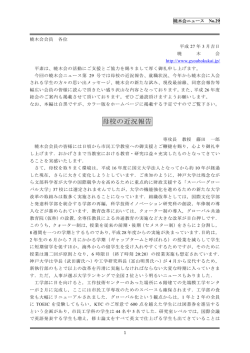
When QGIS starts, you are presented with the GUI as shown in the figure (the numbers 1 through 5 in yellow
circles are discussed below).
Figure 7.1: QGIS GUI with Alaska sample data
ノート: ウィンドウの装飾（タイトルバーとか）は利用している オペレーティングシステムやウィンドウ
マネージャによって見かけが異なります.
The QGIS GUI is divided into five areas:
1. メニューバー
2. Tool Bar
3. Map Legend
4. 地図ビュー
5. ステータスバー
These five components of the QGIS interface are described in more detail in the following sections. Two more
sections present keyboard shortcuts and context help.
21
QGIS User Guide, リリース 2.8
7.1 メニューバー
The menu bar provides access to various QGIS features using a standard hierarchical menu. The top-level menus
and a summary of some of the menu options are listed below, together with the associated icons as they appear on
the toolbar, and keyboard shortcuts. The shortcuts presented in this section are the defaults; however, keyboard
shortcuts can also be configured manually using the Configure shortcuts dialog, opened from Settings → Configure
Shortcuts....
ほとんどのメニューオプションはツールに対応しているけど, 逆に対応していないこともあります, メニュー
はツールバーのようには構成されていません. ツールバーはそれぞれのチェックボックスエントリとしてあ
らわされているメニューオプションのリストツールを含んでいます. いくつかのメニューオプションは対応
するプラグインがロードされている時のみ表示されます. ツールとツールバーについてのさらに詳しい情報
は ツールバー 節を参照して下さい.
7.1.1 プロジェクト
メニューオプション
ショートカット
リファレンス
ツールバー
Ctrl+N
see プロジェクト
プロジェクト
Ctrl+O
see プロジェクト
see プロジェクト
see プロジェクト
プロジェクト
プロジェクト
Save
Ctrl+S
see プロジェクト
プロジェクト
Save As...
Ctrl+Shift+S
see プロジェクト
プロジェクト
New
Open
テンプレートを基に新規作成 →
Open Recent →
see 出力
see 出力
Save as Image...
DXF Export ...
New Print Composer
Ctrl+P
Composer manager ...
プリントコンポーザ →
Exit QGIS
22
see プリントコンポーザ
プロジェクト
see プリントコンポーザ
see プリントコンポーザ
プロジェクト
Ctrl+Q
Chapter 7. QGIS GUI
QGIS User Guide, リリース 2.8
7.1. メニューバー
23
QGIS User Guide, リリース 2.8
7.1.2 編集
メニューオプション
ショートカッ
ト
リファレンス
ツールバー
Undo
Ctrl+Z
see 高度なデジタイジング
先進的なデジタ
イズ
Redo
Ctrl+Shift+Z see 高度なデジタイジング
先進的なデジタ
イズ
Cut Features
Ctrl+X
see 既存レイヤのデジタイズ
デジタジング
Copy Features
Ctrl+C
see 既存レイヤのデジタイズ
デジタジング
Ctrl+V
see 既存レイヤのデジタイズ
Working with the Attribute Table
参照
デジタジング
Ctrl+.
see 既存レイヤのデジタイズ
デジタジング
Move Feature(s)
see 既存レイヤのデジタイズ
デジタジング
Delete Selected
see 既存レイヤのデジタイズ
デジタジング
Rotate Feature(s)
see 高度なデジタイジング
先進的なデジタ
イズ
Simplify Feature
see 高度なデジタイジング
先進的なデジタ
イズ
Add Ring
see 高度なデジタイジング
先進的なデジタ
イズ
Add Part
see 高度なデジタイジング
先進的なデジタ
イズ
Fill Ring
see 高度なデジタイジング
先進的なデジタ
イズ
Delete Ring
see 高度なデジタイジング
先進的なデジタ
イズ
Delete Part
see 高度なデジタイジング
先進的なデジタ
イズ
Reshape Features
see 高度なデジタイジング
先進的なデジタ
イズ
Offset Curve
see 高度なデジタイジング
先進的なデジタ
イズ
Split Features
see 高度なデジタイジング
先進的なデジタ
イズ
Split Parts
see 高度なデジタイジング
先進的なデジタ
イズ
Merge Selected Features
see 高度なデジタイジング
先進的なデジタ
イズ
see 高度なデジタイジング
先進的なデジタ
イズ
Node Tool
see 既存レイヤのデジタイズ
デジタジング
Rotate Point Symbols
see 高度なデジタイジング
先進的なデジタ
イズ
Paste Features
新規レイヤへの地物貼り付け
→
Add Feature
Merge Attr. of Selected
Features
24
Chapter 7. QGIS GUI
QGIS User Guide, リリース 2.8
Toggle editing
After activating
mode for a layer, you will find the Add Feature icon in the Edit menu depending on the layer type (point, line or polygon).
7.1.3 編集（おまけ）
メニューオプション
ショートカット
リファレンス
ツールバー
Add Feature
see 既存レイヤのデジタイズ
デジタジング
Add Feature
see 既存レイヤのデジタイズ
デジタジング
Add Feature
see 既存レイヤのデジタイズ
デジタジング
7.1.4 ビュー
メニューオプション
ショートカット
リファレンス
ツールバー
Pan Map
地図ナビゲーション
Pan Map to Selection
地図ナビゲーション
Zoom In
Zoom Out
選択 →
Ctrl+-
Identify Features
計測 →
Ctrl+Shift+I
Zoom Full
地図ナビゲーション
Ctrl++
see 地物の選択と選択解除
地図ナビゲーション
属性
see 計測
属性
属性
地図ナビゲーション
Ctrl+Shift+F
地図ナビゲーション
Zoom To Layer
Zoom To Selection
地図ナビゲーション
Ctrl+J
Zoom Last
地図ナビゲーション
Zoom Next
地図ナビゲーション
地図ナビゲーション
Zoom Actual Size
地図整飾 →
Preview mode →
整飾 参照
属性
Map Tips
New Bookmark
Ctrl+B
see 空間ブックマーク
属性
Show Bookmarks
Ctrl+Shift+B
see 空間ブックマーク
属性
Refresh
F5
7.1. メニューバー
地図ナビゲーション
25
QGIS User Guide, リリース 2.8
7.1.5 レイヤ
メニューオプション
Create Layer →
Add Layer →
Embed Layers and Groups ...
Add from Layer Definition File ...
ショートカット
リファレンス
新しいベクタレイヤの作成 を参照
ツールバー
レイヤの管理
レイヤの管理
see プロジェクトの入れ子
Copy style
see スタイルメニュー
Paste style
see スタイルメニュー
Open Attribute Table
Working with the Attribute Table 参照
属性
Toggle Editing
see 既存レイヤのデジタイズ
デジタジング
Save Layer Edits
see 既存レイヤのデジタイズ
デジタジング
see 既存レイヤのデジタイズ
デジタジング
Current Edits →
Save as...
Save as layer definition file...
Remove Layer/Group
Ctrl+D
Duplicate Layers (s)
Set Scale Visibility of Layers
Set CRS of Layer(s)
Set project CRS from Layer
Properties ...
Query...
Ctrl+Shift+C
Labeling
Ctrl+Shift+O
レイヤの管理
Show All Layers
Ctrl+Shift+U
レイヤの管理
Hide All Layers
Ctrl+Shift+H
レイヤの管理
Add to Overview
Add All To Overview
Remove All From Overview
Show selected Layers
Hide selected Layers
7.1.6 設定
メニューオプション
パネル →
ツールバー →
Toggle Full Screen Mode
Project Properties ...
Custom CRS ...
スタイルマネージャ...
Configure shortcuts ...
Customization ...
Options ...
Snapping Options ...
26
ショートカット
リファレンス
see Panels and Toolbars
see Panels and Toolbars
ツールバー
F 11
Ctrl+Shift+P
see プロジェクト
see カスタム空間参照システム
see Presentation
see カスタマイゼーション
オプション 参照
Chapter 7. QGIS GUI
QGIS User Guide, リリース 2.8
7.1.7 プラグイン
メニューオプション
ショートカット
Manage and Install Plugins ...
Python Console
Ctrl+Alt+P
リファレンス
ツールバー
see プラグインダイアログ
When starting QGIS for the first time not all core plugins are loaded.
7.1.8 ベクタ
メニューオプション
オープンストリートマップ →
ショートカット
リファレンス
see OpenStreetMap ベクタの読み込み
解析ツール →
see fTools プラグイン
調査ツール →
see fTools プラグイン
ジオプロセッシングツール →
see fTools プラグイン
ジオメトリツール →
see fTools プラグイン
データマネジメントツール →
see fTools プラグイン
ツールバー
When starting QGIS for the first time not all core plugins are loaded.
7.1.9 ラスタ
メニューオプション
Raster calculator ...
ショートカット
リファレンス
see ラスタ計算機
ツールバー
When starting QGIS for the first time not all core plugins are loaded.
7.1.10 Database
メニューオプション
Database →
ショートカット
リファレンス
see DB マネージャプラグイン
ツールバー
Database
When starting QGIS for the first time not all core plugins are loaded.
7.1.11 Web
メニューオプション
Metasearch
ショートカット
リファレンス
see MetaSearch Catalogue Client
ツールバー
Web
When starting QGIS for the first time not all core plugins are loaded.
7.1. メニューバー
27
QGIS User Guide, リリース 2.8
7.1.12 プロセシング
メニューオプション
ショートカット
リファレンス
ツールバー
Toolbox
see ツールボックス
Graphical Modeler ...
グラフィカルモデラー 参照
see 履歴マネージャ
History and log ...
Options ...
プロセッシングフレームワークを構成する 参照
Results viewer ...
see 外部アプリケーションの設定
Commander
Ctrl+Alt+M
QGIS コマンダー 参照
When starting QGIS for the first time not all core plugins are loaded.
7.1.13 ヘルプ
メニューオプション
ショートカット
Help Contents
What’s This?
API Documentation
Need commercial support?
QGIS Home Page
リファレンス
ツールバー
F1
ヘルプ
Shift+F1
ヘルプ
Ctrl+H
Check QGIS Version
About
QGIS Sponsors
Please note that for Linux , the menu bar items listed above are the default ones in the KDE window manager.
In GNOME, the Settings menu has different content and its items have to be found here:
Custom CRS
Style Manager
Configure Shortcuts
Customization
Options
Snapping Options ...
Edit
Edit
Edit
Edit
Edit
Edit
7.2 ツールバー
ツールバーではメニューのほとんどと同じ機能を提供している上に対話的に地図を操作する機能を提供し
ています. ツールバーのそれぞれのアイテムではポップアップヘルプが提供されています. マウスでアイテ
ムの上を動かすとツールの簡単な説明が表示されます.
Every menu bar can be moved around according to your needs. Additionally, every menu bar can be switched off
using your right mouse button context menu, holding the mouse over the toolbars (read also Panels and Toolbars).
ちなみに: ツールバーの復元
If you have accidentally hidden all your toolbars, you can get them back by choosing menu option Settings →
Toolbars →. If a toolbar disappears under Windows, which seems to be a problem in QGIS from time to time, you
have to remove key \HKEY_CURRENT_USER\Software\QGIS\qgis\UI\state in the registry. When
you restart QGIS, the key is written again with the default state, and all toolbars are visible again.
28
Chapter 7. QGIS GUI
QGIS User Guide, リリース 2.8
7.3 Map Legend
The map legend area lists all the layers in the project. The checkbox in each legend entry can be used to show or
hide the layer. The Legend toolbar in the map legend are list allow you to Add group, Manage Layer Visibility
of all layers or manage preset layers combination, Filter Legend by Map Content, Expand All or Collapse All
and Remove Layer or Group. The button
allows you to add Presets views in the legend. It means that
you can choose to display some layer with specific categorization and add this view to the Presets list. To add a
preset view just click on
, choose Add Preset... from the drop down menu and give a name to the preset.
After that you will see a list with all the presets that you can recall pressing on the
button.
All the added presets are also present in the map composer in order to allow you to create a map layout based on
your specific views (see メインプロパティ).
レイヤは選択してドラッグで上下に移動することによって Z オーダリングを変えることができます.Z オー
ダリングとは, 凡例のリストでの表示順が地図表示のレイヤ表示順になることです.
ノート: This behaviour can be overridden by the ‘Layer order’ panel.
Layers in the legend window can be organised into groups. There are two ways to do this:
1. Press the
icon to add a new group. Type in a name for the group and press Enter. Now click on an
existing layer and drag it onto the group.
2. 凡例ウィンドウでいくつかのレイヤを選択してマウス右ボタンをクリックして Group Selected を選択
して下さい. 選択されたレイヤで自動的に新しいグループが作られます.
あるレイヤをグループからはずしたい場合はレイヤ名をドラッグしてグループ外に持っていくかマウス右
ボタンクリックして Make to toplevel item を選択して下さい. グループは他のグループからネストすること
ができます.
グループ用チェックボックスを使うとグループ内全レイヤの表示, 非表示を 1 回のクリックで行えます.
The content of the right mouse button context menu depends on whether the selected legend item is a raster or a
Toggle editing
vector layer. For GRASS vector layers,
is not available. See section GRASS ベクタレイヤのデジ
タイジングと編集 for information on editing GRASS vector layers.
Right mouse button menu for raster layers
• Zoom to Layer
• Show in overview
• Zoom to Best Scale (100%)
• Remove
• Duplicate
• Set Layer Scale Visibility
• Set Layer CRS
• レイヤの CRS をプロジェクトに設定する
• Styles →
• Save as ...
• Save As Layer Definition File ...
• プロパティ
• 改名
Additionally, according to layer position and selection
7.3. Map Legend
29
QGIS User Guide, リリース 2.8
• Move to Top-level
• 選択されたレイヤをグループにする
Right mouse button menu for vector layers
• Zoom to Layer
• Show in overview
• Remove
• Duplicate
• Set Layer Scale Visibility
• Set Layer CRS
• レイヤの CRS をプロジェクトに設定する
• Styles →
• Open Attribute Table
• Toggle Editing (not available for GRASS layers)
• Save As ...
• Save As Layer Definition Style
• フィルター
• Show Feature Count
• プロパティ
• 改名
Additionally, according to layer position and selection
• Move to Top-level
• 選択されたレイヤをグループにする
Right mouse button menu for layer groups
• Zoom to Group
• Remove
• Set Group CRS
• 改名
• Add Group
It is possible to select more than one layer or group at the same time by holding down the Ctrl key while selecting
the layers with the left mouse button. You can then move all selected layers to a new group at the same time.
You may also delete more than one layer or group at once by selecting several layers with the Ctrl key and
pressing Ctrl+D afterwards. This way, all selected layers or groups will be removed from the layers list.
7.3.1 レイヤの標示順序から独立した凡例の操作
There is a panel that allows you to define an independent drawing order for the map legend. You can activate
it in the menu Settings → Panels → Layer order. This feature allows you to, for instance, order your layers in
order of importance, but still display them in the correct order (see figure_layer_order). Checking the
rendering order box underneath the list of layers will cause a revert to default behavior.
30
Control
Chapter 7. QGIS GUI
QGIS User Guide, リリース 2.8
Figure 7.2: Define a legend independent layer order
7.4 地図ビュー
This is the “business end” of QGIS — maps are displayed in this area! The map displayed in this window will
depend on the vector and raster layers you have chosen to load (see sections that follow for more information on
how to load layers). The map view can be panned, shifting the focus of the map display to another region, and
it can be zoomed in and out. Various other operations can be performed on the map as described in the toolbar
description above. The map view and the legend are tightly bound to each other — the maps in view reflect
changes you make in the legend area.
ちなみに: マウスホィールを使って地図をズームします
マウスホィールを使って地図のズームインとズームアウトを行うことができます. マウスカーソルを地図
エリアの中に置きホィールを前方 (あなたの側から) ロールするとズームインを行えます, そして手前に (あ
なたの側に) ロールするとズームアウトします. マウスカーソルの位置がズームの中心になります. マウス
ホィールのズーム動作については Settings → Options メニューの Map tools タブでカスタマイズができます.
ちなみに: 矢印キーとスペースバーを使った地図パンニング
矢印キーを使ってパンを行うことができます. マウスカーソルを地図エリアにおきクリックした後右矢印
キーを押すと東にパンします, 左矢印キーを押すと西にパンします, 上矢印キーを押すと北にパンします. 下
矢印キーを押すと南にパンします. またスペースバーかマウスホィールを使ってパンを行うことができます.
この場合スペースバーを押しながらマウスを動かすかマウスホィールをクリックして下さい.
7.5 ステータスバー
The status bar shows you your current position in map coordinates (e.g., meters or decimal degrees) as the mouse
pointer is moved across the map view. To the left of the coordinate display in the status bar is a small button that
will toggle between showing coordinate position or the view extents of the map view as you pan and zoom in and
out.
7.4. 地図ビュー
31
QGIS User Guide, リリース 2.8
Next to the coordinate display you will find the scale display. It shows the scale of the map view. If you zoom in or
out, QGIS shows you the current scale. There is a scale selector, which allows you to choose between predefined
scales from 1:500 to 1:1000000.
To the right of the scale display you can define a current clockwise rotation for your map view in degrees.
A progress bar in the status bar shows the progress of rendering as each layer is drawn to the map view. In some
cases, such as the gathering of statistics in raster layers, the progress bar will be used to show the status of lengthy
operations.
If a new plugin or a plugin update is available, you will see a message at the far left of the status bar. On the right
side of the status bar, there is a small checkbox which can be used to temporarily prevent layers being rendered
to the map view (see section レンダリング below). The icon
process.
immediately stops the current map rendering
To the right of the render functions, you find the EPSG code of the current project CRS and a projector icon.
Clicking on this opens the projection properties for the current project.
ちなみに: マップキャンバスにおける正しい縮尺を計算する
When you start QGIS, the default units are degrees, and this means that QGIS will interpret any coordinate in your
layer as specified in degrees. To get correct scale values, you can either change this setting to meters manually in
Current CRS:
the General tab under Settings → Project Properties, or you can select a project CRS clicking on the
icon in the lower right-hand corner of the status bar. In the last case, the units are set to what the project projection
specifies (e.g., ‘+units=m’).
.
32
Chapter 7. QGIS GUI
Chapter 8
一般ツール
8.1 キーボードショートカット
QGIS provides default keyboard shortcuts for many features. You can find them in section メニューバー. Additionally, the menu option Settings → Configure Shortcuts.. allows you to change the default keyboard shortcuts
and to add new keyboard shortcuts to QGIS features.
Figure 8.1: Define shortcut options
(Gnome)
Configuration is very simple. Just select a feature from the list and click on [Change], [Set none] or [Set default].
Once you have finished your configuration, you can save it as an XML file and load it to another QGIS installation.
8.2 コンテキストヘルプ
特定のトピックでヘルプが必要な場合多くのダイアログに実装されている [Help] ボタンでコンテキストヘ
ルプを利用することができます- サードパーティプラグインでは専用のウェッブページを指し示すことを注
意して下さい.
8.3 レンダリング
By default, QGIS renders all visible layers whenever the map canvas is refreshed. The events that trigger a refresh
of the map canvas include:
33
QGIS User Guide, リリース 2.8
• レイヤの追加
• パンまたはズーム
• Resizing the QGIS window
• レイヤまたはレイヤ群の表示、非表示を変更します
QGIS allows you to control the rendering process in a number of ways.
8.3.1 スケール依存レンダリング
スケール依存レンダリングを利用するとあるレイヤが表示される最小と最大のスケールを指定することが
できます. スケール依存レンダリングを設定する場合レイヤを凡例でダブルクリックして プロパティ ダイ
アログを開いて下さい. 一般情報 タブで,
最小と最大の縮尺値を設定して下さい.
縮尺に応じた表示設定 チェックボックスをアクティブにして
You can determine the scale values by first zooming to the level you want to use and noting the scale value in the
QGIS status bar.
8.3.2 地図レンダリングの制御
Map rendering can be controlled in the various ways, as described below.
描画の中断
Render checkbox in the lower right corner of the status bar. When the
To suspend rendering, click the
Render checkbox is not checked, QGIS does not redraw the canvas in response to any of the events described in
section レンダリング. Examples of when you might want to suspend rendering include:
• 沢山のレイヤを追加して描画する前に描画方法を編集したい場合
• データ量が多いレイヤを追加して描画する前に縮尺依存描画条件を指定したい場合
• データ量が多いレイヤを追加して描画する前に特定の位置にズームしておきたい場合
• 上記の場合のいくつかの組み合わせ
Checking the
Render checkbox enables rendering and causes an immediate refresh of the map canvas.
レイヤ追加オプションの設定
新しくレイヤを追加した時に, すぐに描画しないオプションを設定できます. これはレイヤが地図に追加さ
れた時に, 地図凡例の可視属性チェックボックスがデフォルトでチェックされないことを意味します. このオ
プションを指定するためには 設定 → オプション → を選択して レンダリング タブをクリックしてくださ
By default new layers added to the map should be displayed のチェックを解除してください. すると, 地
い.
図に追加されたレイヤの表示属性は不可視の状態がデフォルトになります.
描画の中断
地図描画を中断したい場合は ESC キーを押して下さい. これにより地図キャンパスの更新が中断され地図
の一部が描画された状態になります. ESC キーを押してから地図描画が中断されるまで少し時間がかかり
ます.
ノート: 現在描画中断機能は利用できません - これは Qt4 のポートに依存しています, なぜならばユーザー
インターフェース (UI) に問題が発生してクラッシュするからです.
34
Chapter 8. 一般ツール
QGIS User Guide, リリース 2.8
Updating the Map Display During Rendering
You can set an option to update the map display as features are drawn. By default, QGIS does not display any
features for a layer until the entire layer has been rendered. To update the display as features are read from the
datastore, choose menu option Settings → Options and click on the Rendering tab. Set the feature count to an
appropriate value to update the display during rendering. Setting a value of 0 disables update during drawing (this
is the default). Setting a value too low will result in poor performance, as the map canvas is continually updated
during the reading of the features. A suggested value to start with is 500.
描画品質への影響
To influence the rendering quality of the map, you have two options. Choose menu option Settings → Options,
click on the Rendering tab and select or deselect following checkboxes:
•
Make lines appear less jagged at the expense of some drawing performance
•
Fix problems with incorrectly filled polygons
スピードアップレンダリング
There are two settings that allow you to improve rendering speed. Open the QGIS options dialog using Settings
→ Options, go to the Rendering tab and select or deselect the following checkboxes:
•
•
Enable back buffer. This provides better graphics performance at the cost of losing the possibility to
cancel rendering and incrementally draw features. If it is unchecked, you can set the Number of features to
draw before updating the display, otherwise this option is inactive.
再描画の速度を上げられる場合にレンダのキャッシュを利用します
8.4 計測
Measuring works within projected coordinate systems (e.g., UTM) and unprojected data. If the loaded map is
defined with a geographic coordinate system (latitude/longitude), the results from line or area measurements will
be incorrect. To fix this, you need to set an appropriate map coordinate system (see section 投影法の利用方法).
All measuring modules also use the snapping settings from the digitizing module. This is useful, if you want to
measure along lines or areas in vector layers.
To select a measuring tool, click on
and select the tool you want to use.
8.4.1 Measure length, areas and angles
Measure Line
: QGIS is able to measure real distances between given points according to a defined ellipsoid.
To configure this, choose menu option Settings → Options, click on the Map tools tab and select the appropriate
ellipsoid. There, you can also define a rubberband color and your preferred measurement units (meters or feet) and
angle units (degrees, radians and gon). The tool then allows you to click points on the map. Each segment length,
as well as the total, shows up in the measure window. To stop measuring, click your right mouse button. Note
that you can interactively change the measurement units in the measurement dialog. It overrides the Preferred
measurement units in the options. There is an info section in the dialog that shows which CRS settings are being
used during measurement calculations.
Measure Area
: Areas can also be measured. In the measure window, the accumulated area size appears. In
addition, the measuring tool will snap to the currently selected layer, provided that layer has its snapping tolerance
set (see section スナップ許容量と検索半径の設定). So, if you want to measure exactly along a line feature, or
8.4. 計測
35
QGIS User Guide, リリース 2.8
Figure 8.2: Measure Distance
(Gnome)
around a polygon feature, first set its snapping tolerance, then select the layer. Now, when using the measuring
tools, each mouse click (within the tolerance setting) will snap to that layer.
Figure 8.3: Measure Area
(Gnome)
Measure Angle
: You can also measure angles. The cursor becomes cross-shaped. Click to draw the first segment
of the angle you wish to measure, then move the cursor to draw the desired angle. The measure is displayed in a
pop-up dialog.
Figure 8.4: Measure Angle
(Gnome)
8.4.2 地物の選択と選択解除
The QGIS toolbar provides several tools to select features in the map canvas. To select one or several features,
just click on
and select your tool:
•
Select Single Feature
•
Select Features by Rectangle
•
Select Features by Polygon
•
Select Features by Freehand
•
Select Features by Radius
To deselect all selected features click on
36
Deselect features from all layers
.
Chapter 8. 一般ツール
QGIS User Guide, リリース 2.8
Select feature using an expression
allow user to select feature using expression dialog. See Expressions chapter for
some example.
Users can save features selection into a New Memory Vector Layer or a New Vector Layer using Edit → Paste
Feature as ... and choose the mode you want.
8.5 地物情報表示
The Identify tool allows you to interact with the map canvas and get information on features in a pop-up window.
To identify features, use View → Identify features or press Ctrl + Shift + I, or click on the
icon in the toolbar.
Identify features
If you click on several features, the Identify results dialog will list information about all the selected features. The
first item is the number of the layer in the list of results, followed by the layer name. Then, its first child will be the
name of a field with its value. The first field is the one selected in Properties → Display. Finally, all information
about the feature is displayed.
このウィンドウはカスタムフィールドを表示するためにカスタマイズできますがデフォルトで 3 種類の情
報を表示します:
• Actions: Actions can be added to the identify feature windows. When clicking on the action label, action
will be run. By default, only one action is added, to view feature form for editing.
• Derived: This information is calculated or derived from other information. You can find clicked coordinate,
X and Y coordinates, area in map units and perimeter in map units for polygons, length in map units for
lines and feature ids.
• Data attributes: This is the list of attribute fields from the data.
Figure 8.5: Identify feaures dialog
(Gnome)
At the top of the window, you have five icons:
•
Expand tree
•
Collapse tree
•
Default behaviour
•
Copy attributes
•
Print selected HTML response
8.5. 地物情報表示
37
QGIS User Guide, リリース 2.8
At the bottom of the window, you have the Mode and View comboboxes. With the Mode combobox you can define
the identify mode: ‘Current layer’, ‘Top down, stop at first’, ‘Top down’ and ‘Layer selection’. The View can be
set as ‘Tree’, ‘Table’ and ‘Graph’.
The identify tool allows you to auto open a form. In this mode you can change the feautures attributes.
その他の機能は、識別されたアイテムのコンテキストメニューにあります。たとえば、コンテキストメニュー
から次のことができます：
• 地物フォームの表示
• 地物のズーム
• 地物のコピー: すべての地物, のジオメトリと属性をコピーします;
• Toggle feature selection: adds identified feature to selection
• 属性値のコピー: あなたがクリックした属性値のみをコピーします。
• Copy feature attributes: Copy only attributes
• 結果のクリア:ウィンドウ内の結果が削除されます
• ハイライトのクリア:地図上でハイライトしている地物が除去されます
• すべてをハイライトする
• レイヤをハイライトする
• レイヤのアクティベート: アクティベートするレイヤの選択
• レイヤプロパティ: レイヤプロパティウィンドウを表示する
• すべてを展開する
• すべてを折りたたむ
8.6 整飾
The Decorations of QGIS include the Grid, the Copyright Label, the North Arrow and the Scale Bar. They are
used to ‘decorate’ the map by adding cartographic elements.
8.6.1 グリッド
グリッド
では座標のグリッドと座標注記をマップキャンバスに追加します。
1. Select from menu View → Decorations → Grid. The dialog starts (see figure_decorations_1).
2. マップキャンバスにロードされているレイヤにしたがって
してグリッドの設定を行って下さい.
Enable grid チェックボックスを有効に
3. マップキャンバスにロードされているレイヤにしたがって
有効にしてアノテーションの定義を行ってください.
Draw annotations チェックボックスを
4. Click [Apply] to verify that it looks as expected.
5. Click [OK] to close the dialog.
8.6.2 著作権ラベル
Copyright label
adds a copyright label using the text you prefer to the map.
1. メニューの ビュー → 地図整飾 → 著作権ラベル を選択します。ダイアログが表示されます ( figure_decorations_2 を参照すること)。
38
Chapter 8. 一般ツール
QGIS User Guide, リリース 2.8
Figure 8.6: The Grid Dialog
Figure 8.7: The Copyright Dialog
8.6. 整飾
39
QGIS User Guide, リリース 2.8
2. マップ上に配置したいテキストを入力してください. 例に示す通り HTML を使用することができます.
3. Choose the placement of the label from the Placement
4. Make sure the
combo box.
Enable Copyright Label checkbox is checked.
5. Click [OK].
In the example above, which is the default, QGIS places a copyright symbol followed by the date in the lower
right-hand corner of the map canvas.
8.6.3 北向き矢印
North Arrow
places a simple north arrow on the map canvas. At present, there is only one style available. You
can adjust the angle of the arrow or let QGIS set the direction automatically. If you choose to let QGIS determine
the direction, it makes its best guess as to how the arrow should be oriented. For placement of the arrow, you have
four options, corresponding to the four corners of the map canvas.
Figure 8.8: The North Arrow Dialog
8.6.4 スケールバー
Scale Bar
adds a simple scale bar to the map canvas. You can control the style and placement, as well as the
labeling of the bar.
Figure 8.9: The Scale Bar Dialog
QGIS only supports displaying the scale in the same units as your map frame. So if the units of your layers are in
meters, you can’t create a scale bar in feet. Likewise, if you are using decimal degrees, you can’t create a scale
bar to display distance in meters.
40
Chapter 8. 一般ツール
QGIS User Guide, リリース 2.8
スケールバーを追加するために：
1. メニューの ビュー → 地図整飾 → 著作権ラベル を選択して下さい. ダイアログが表示されます (
figure_decorations_4 を参照して下さい).
2. Choose the placement from the Placement
3. Choose the style from the Scale bar style
combo box.
combo box.
4. Select the color for the bar Color of bar
5. Set the size of the bar and its label Size of bar
6. Make sure the
or use the default black color.
.
Enable scale bar checkbox is checked.
7. Optionally, check
Automatically snap to round number on resize.
8. Click [OK].
ちなみに: 整飾の設定
.qgs プロジェクトを保存する際, グリッド, 方位記号, スケールバーと著作権ラベルに加えた変更はそのプ
ロジェクトに保存され, 次回プロジェクトをロードした際に復元されます.
8.7 アノテーションツール
Text Annotation
The
tool in the attribute toolbar provides the possibility to place formatted text in a balloon on the
QGIS map canvas. Use the Text Annotation tool and click into the map canvas.
Figure 8.10: Annotation text dialog
項目をダブルクリックすると、さまざまなオプションを含むダイアログが開きます。フォーマットされた
テキストやその他の項目の設定値を入力するテキストエディタがあります。例えば、マップの位置（マー
カーシンボルが表示された）に関する項目またはスクリーンの位置（マップに関連していない）における
選択肢を持ちます。この項目はマップの位置（マップマーカーをドラッグすることにより）が移動し、ま
たはバルーンのみが移動します。アイコンは、GIS の主題図の一部であり、それらも、他の主題図におい
てデフォルトとして用いられます。
The
Move Annotation
tool allows you to move the annotation on the map canvas.
8.7. アノテーションツール
41
QGIS User Guide, リリース 2.8
8.7.1 HTML 注記
Html Annotation
The
tools in the attribute toolbar provides the possibility to place the content of an html file in a
balloon on the QGIS map canvas. Using the Html Annotation tool, click into the map canvas and add the path to
the html file into the dialog.
8.7.2 SVG 注記
SVG Annotation
The
tool in the attribute toolbar provides the possibility to place an SVG symbol in a balloon on
the QGIS map canvas. Using the SVG Annotation tool, click into the map canvas and add the path to the SVG file
into the dialog.
8.7.3 注記の書式設定
Form Annotation
Additionally, you can also create your own annotation forms. The
tool is useful to display
attributes of a vector layer in a customized Qt Designer form (see figure_custom_annotation). This is similar
to the designer forms for the Identify features tool, but displayed in an annotation item. Also see this video
https://www.youtube.com/watch?v=0pDBuSbQ02o from Tim Sutton for more information.
Figure 8.11: Customized qt designer annotation form
ノート: If you press Ctrl+T while an Annotation tool is active (move annotation, text annotation, form annotation), the visibility states of the items are inverted.
8.8 空間ブックマーク
Spatial Bookmarks allow you to “bookmark” a geographic location and return to it later.
42
Chapter 8. 一般ツール
QGIS User Guide, リリース 2.8
8.8.1 ブックマークの作成
ブックマークを作るには：
1. 関心のある領域にズームまたはパンします。
2. Select the menu option View → New Bookmark or press Ctrl-B.
3. ブックマークを説明する名称（255 文字まで）を入力します。
4. Press Enter to add the bookmark or [Delete] to remove the bookmark.
同じ名称で複数のブックマークを所有できることにご注意ください。
8.8.2 ブックマークの操作
To use or manage bookmarks, select the menu option View → Show Bookmarks. The Geospatial Bookmarks
dialog allows you to zoom to or delete a bookmark. You cannot edit the bookmark name or coordinates.
8.8.3 Zooming to a Bookmark
From the Geospatial Bookmarks dialog, select the desired bookmark by clicking on it, then click [Zoom To]. You
can also zoom to a bookmark by double-clicking on it.
8.8.4 Deleting a Bookmark
To delete a bookmark from the Geospatial Bookmarks dialog, click on it, then click [Delete]. Confirm your choice
by clicking [Yes], or cancel the delete by clicking [No].
8.8.5 Import or export a bookmark
To share or transfer your bookmarks between computers you can use the Share pull down menu in the Geospatial
Bookmarks dialog.
8.9 プロジェクトの入れ子
あなたのプロジェクトに他のプロジェクトファイルからコンテンツを埋め込む場合 Layer → 埋め込みレイ
ヤとグループ を選択して下さい.
8.9.1 埋め込みレイヤ
次のダイアログで, 他のプロジェクトのレイヤを埋め込むことができます.
1. Press
to look for another project from the Alaska dataset.
2. Select the project file grassland. You can see the content of the project (see figure_embed_dialog).
3. Press Ctrl and click on the layers grassland and regions. Press [OK]. The selected layers are
embedded in the map legend and the map view now.
埋め込まれているレイヤが編集可能になっている間, スタイルやラベリングのようなプロパティは変更する
ことができません.
8.9. プロジェクトの入れ子
43
QGIS User Guide, リリース 2.8
Figure 8.12: Select layers and groups to embed
8.9.2 埋め込みレイヤの除去
Right-click on the embedded layer and choose
Remove
.
.
44
Chapter 8. 一般ツール
Chapter 9
QGIS Configuration
QGIS is highly configurable through the Settings menu. Choose between Panels, Toolbars, Project Properties,
Options and Customization.
ノート: QGIS follows desktop guidelines for the location of options and project properties item. Consequently
related to the OS you are using, location of some of items described above could be located in the View menu
(Panels and Toolbars) or in Project for Options.
9.1 Panels and Toolbars
In the Panels→ menu, you can switch on and off QGIS widgets. The Toolbars→ menu provides the possibility to
switch on and off icon groups in the QGIS toolbar (see figure_panels_toolbars).
Figure 9.1: The Panels and Toolbars menu
45
QGIS User Guide, リリース 2.8
ちなみに: Activating the QGIS Overview
In QGIS, you can use an overview panel that provides a full extent view of layers added to it. It can be selected
under the menu
Settings → Panels or
View → Panels. Within the view is a rectangle showing the current
map extent. This allows you to quickly determine which area of the map you are currently viewing. Note that
labels are not rendered to the map overview even if the layers in the map overview have been set up for labeling.
If you click and drag the red rectangle in the overview that shows your current extent, the main map view will
update accordingly.
ちなみに: Show Log Messages
It’s possible to track the QGIS messages. You can activate
Log Messages in the menu
Settings → Panels
or View → Panels and follow the messages that appear in the different tabs during loading and operation.
9.2 プロジェクトのプロパティ
In the properties window for the project under Settings → Project Properties (kde) or
Properties (Gnome), you can set project-specific options. These include:
Project → Project
• In the General menu, the project title, selection and background color, layer units, precision, and the option
to save relative paths to layers can be defined. If the CRS transformation is on, you can choose an ellipsoid
for distance calculations. You can define the canvas units (only used when CRS transformation is disabled)
and the precision of decimal places to use. You can also define a project scale list, which overrides the
global predefined scales.
• The CRS menu enables you to choose the Coordinate Reference System for this project, and to enable
on-the-fly re-projection of raster and vector layers when displaying layers from a different CRS.
• With the third Identify layers menu, you set (or disable) which layers will respond to the identify tool (see
the “Map tools” paragraph from the オプション section to enable identifying of multiple layers).
• The Default Styles menu lets you control how new layers will be drawn when they do not have an existing
.qml style defined. You can also set the default transparency level for new layers and whether symbols
should have random colours assigned to them. There is also an additional section where you can define
specific colors for the running project. You can find the added colors in the drop down menu of the color
dialog window present in each renderer.
• The tab OWS Server allows you to define information about the QGIS Server WMS and WFS capabilities,
extent and CRS restrictions.
• マクロ メニューは Python マクロの編集のために使います. 現時点では: openProject(),
saveProject() そして closeProject() の 3 つのマクロのみ使用可能です.
• The Relations menu is used to define 1:n relations. The relations are defined in the project properties dialog.
Once relations exist for a layer, a new user interface element in the form view (e.g. when identifying a
feature and opening its form) will list the related entities. This provides a powerful way to express e.g. the
inspection history on a length of pipeline or road segment. You can find out more about 1:n relations support
in Section Creating one to many relations.
9.3 オプション
Some basic options for QGIS can be selected using the Options dialog. Select the menu option Settings →
Options. The tabs where you can customize your options are described below.
46
Chapter 9. QGIS Configuration
QGIS User Guide, リリース 2.8
Figure 9.2: Macro settings in QGIS
9.3.1 一般情報メニュー
アプリケーション
• Select the Style (QGIS restart required)
‘Plastique’ and ‘Cleanlooks’ ( ).
• Define the Icon theme
and choose between ‘Oxygen’,’Windows’,’Motif’,’CDE’,
. Currently only ‘default’ is possible.
• Define the Icon size
.
• Define the Font. Choose between
Qt default and a user-defined font.
• Change the Timeout for timed messages or dialogs
.
•
起動時のスプラッシュスクリーンを隠す
•
起動時にチップスを表示する
•
グループボックスのタイトルを太字にする
•
QGIS スタイルのグループボックス
•
Use native color chooser dialogs
•
Use live-updating color chooser dialogs
•
Custom side bar style
•
Experimental canvas rotation support (restart required)
プロジェクトファイル
• Open project on launch
‘Specific’ use the
•
(choose between ‘New’, ‘Most recent’ and ‘Specific’). When choosing
to define a project.
既定のプロジェクトから新プロジェクトを作成する. 現在のプロジェクトを既定プロジェクトとし
て指定する または 既定を解除 ボタンをクリックすることができます. またユーザが作成したプロジェ
クトテンプレートをファイルやディレクトリを指定するとブラウズすることができます. プロジェク
9.3. オプション
47
QGIS User Guide, リリース 2.8
ト → テンプレートをもとに新規作成 というエントリでそれができます. プロジェクトテンプレート
を保存したい場合は最初に
既定のプロジェクトから新プロジェクトを作成する をアクティブにし
てプロジェクトテンプレートフォルダーにプロジェクトを保存してください.
•
必要に応じプロジェクトとデータソースの変更の保存を促す
•
Prompt for confirmation when a layer is to be removed
•
QGIS の旧バージョンで保存したプロジェクトファイルを開く際に警告する
• Enable macros
. This option was created to handle macros that are written to perform an action on
project events. You can choose between ‘Never’, ‘Ask’, ‘For this session only’ and ‘Always (not recommended)’.
9.3.2 システムメニュー
環境
System environment variables can now be viewed, and many configured, in the Environment group (see figure_environment_variables). This is useful for platforms, such as Mac, where a GUI application does not necessarily inherit the user’s shell environment. It’s also useful for setting and viewing environment variables for
the external tool sets controlled by the Processing toolbox (e.g., SAGA, GRASS), and for turning on debugging
output for specific sections of the source code.
•
Use custom variables (restart required - include separators). You can [Add] and [Remove] variables.
Already-defined environment variables are displayed in Current environment variables, and it’s possible to
filter them by activating
Show only QGIS-specific variables.
Figure 9.3: System environment variables in QGIS
プラグインパス
[Add] or [Remove] Path(s) to search for additional C++ plugin libraries
48
Chapter 9. QGIS Configuration
QGIS User Guide, リリース 2.8
9.3.3 データソースメニュー
地物属性とテーブル
•
•
ドックウィンドウで属性テーブルを開く（QGIS の再起動が必要）‘
Copy selected rows to clipboard
Copy geometry in WKT representation from attribute table. When using
from the Attribute table dialog, this has the result that the coordinates of points or vertices are also copied
to the clipboard.
• Attribute table behaviour
. There are three possibilities: ‘Show all features’, ‘Show selected features’
and ‘Show features visible on map’.
• Attribute table row cache
. This row cache makes it possible to save the last loaded N attribute rows
so that working with the attribute table will be quicker. The cache will be deleted when closing the attribute
table.
• Representation for NULL values. Here, you can define a value for data fields containing a NULL value.
データソースの操作
• Scan for valid items in the browser dock
contents’.
. You can choose between ‘Check extension’ and ‘Check file
• Scan for contents of compressed files (.zip) in browser dock
possible.
. ‘No’, ‘Basic scan’ and ‘Full scan’ are
• Prompt for raster sublayers when opening. Some rasters support sublayers — they are called subdatasets
in GDAL. An example is netCDF files — if there are many netCDF variables, GDAL sees every variable
as a subdataset. The option allows you to control how to deal with sublayers when a file with sublayers is
opened. You have the following choices:
– ‘ 常に ’:毎回確認 (サブレイヤが存在する場合)
– ‘ 必要な場合 ’:バンドがなくサブレイヤをもつかを尋ねます
– ‘ 利用しない ’:確認せず何もロードしません
– ‘‘ すべてをロード’:確認せず, すべてのサブレイヤをロードします
•
Ignore shapefile encoding declaration. If a shapefile has encoding information, this will be ignored by
QGIS.
•
Add PostGIS layers with double click and select in extended mode
•
ダブルクリックで Oracle レイヤを追加する. 拡張選択モードを利用する
9.3.4 レンダリングメニュー
Rendering behaviour
•
地図に新しくレイヤを追加した際にそのレイヤが表示されることをデフォルトにする
•
再描画の速度を上げられる場合にレンダのキャッシュを利用します
•
Render layers in parallel using many CPU cores
•
Max cores to use
• Map update interval (default to 250 ms)
•
Enable feature simplication by default for newly added layers
• Simplification threshold
9.3. オプション
49
QGIS User Guide, リリース 2.8
可能であればプロバイダ側で簡素化
•
• Maximum scale at which the layer should be simplified
描画品質
線のジャギーを目立たなくします (描画パフォーマンスが低下します)
•
ラスタ
• With RGB band selection, you can define the number for the Red, Green and Blue band.
Contrast enhancement
• Single band gray
. A single band gray can have ‘No stretch’, ‘Stretch to MinMax’, ‘Stretch and Clip
to MinMax’ and also ‘Clip to MinMax’.
• Multi band color (byte/band)
MinMax’ and ‘Clip to MinMax’.
. Options are ‘No stretch’, ‘Stretch to MinMax’, ‘Stretch and Clip to
• Multi band color (>byte/band)
MinMax’ and ‘Clip to MinMax’.
. Options are ‘No stretch’, ‘Stretch to MinMax’, ‘Stretch and Clip to
• Limits (minimum/maximum)
‘Mean +/- standard deviation’.
. Options are ‘Cumulative pixel count cut’, ‘Minimum/Maximum’,
• 累積ピクセル数のカット制限
• 標準偏差の乗数
デバッグ
•
マップキャンバスリフレッシュ
9.3.5 Colors Menu
This menu allows you to add some custom color that you can find in each color dialog window of the renderers.
You will see a set of predefined colors in the tab: you can delete or edit all of them. Moreover you can add the
color you want and perform some copy and paste operations. Finally you can export the color set as a gpl file or
import them.
9.3.6 キャンバスと凡例のメニュー
デフォルトのマップ外観（プロジェクトプロパティを上書きします）
• Define a Selection color and a Background color.
レイヤの凡例
• Double click action in legend
the double click.
. You can either ‘Open layer properties’ or ‘Open attribute table’ with
• 以下の 凡例アイテムスタイル は利用可能です
50
–
レイヤ名の最初を大文字にする
–
レイヤ名を太字にする
–
グループ名を太字にする
–
分類の属性名称を表示する
–
ラスタアイコンの作成 (多分遅い)
Chapter 9. QGIS Configuration
QGIS User Guide, リリース 2.8
9.3.7 マップツールズメニュー
This menu offers some options regarding the behaviour of the Identify tool.
• Search radius for identifying and displaying map tips is a tolerance factor expressed as a percentage of the
map width. This means the identify tool will depict results as long as you click within this tolerance.
• Highlight color allows you to choose with which color should features being identified are to be highlighted.
• Buffer expressed as a percentage of the map width, determines a buffer distance to be rendered from the
outline of the identify highlight.
• Minimum width expressed as a percentage of the map width, determines how thick should the outline of a
highlighted object be.
計測ツール
• 計測ツールの ラバーバンド色 を定義します。
• Define 小数位
•
Keep base unit
• Preferred measurements units
• Preferred angle units
(‘Meters’, ‘Feet’, ‘Nautical Miles’ or ‘Degrees’)‘
(‘Degrees’, ‘Radians’ or ‘Gon’)
パンとズーム
• Define Mouse wheel action
(‘Zoom’, ‘Zoom and recenter’, ‘Zoom to mouse cursor’, ‘Nothing’)
• ホイールマウスの ズーム倍率 の定義
定義済み縮尺
Here, you find a list of predefined scales. With the [+] and [-] buttons you can add or remove your individual
scales.
9.3.8 コンポーザメニュー
コンポジションデフォルト
You can define the Default font here.
グリッドの外観
• Define the Grid style
(‘Solid’, ‘Dots’, ‘Crosses’)
• Define the Grid color
Grid and guide defaults
• Define the Grid spacing
• Define the Grid offset
for x and y
• Define the Snap tolerance
9.3.9 デジタイズメニュー
地物の作成
•
地物作成後のポップアップ属性入力を行わない
•
最後に入力した値を再利用する
9.3. オプション
51
QGIS User Guide, リリース 2.8
• Validate geometries. Editing complex lines and polygons with many nodes can result in very slow rendering.
This is because the default validation procedures in QGIS can take a lot of time. To speed up rendering, it is
possible to select GEOS geometry validation (starting from GEOS 3.3) or to switch it off. GEOS geometry
validation is much faster, but the disadvantage is that only the first geometry problem will be reported.
ラバーバンド
• ラバーバンドの 線幅 と 線色 を指定して下さい
スナップ
•
ドックウィンドウ内でスナップオプションを開く (QGIS の再起動が必要)
• Define Default snap mode
(‘To vertex’, ‘To segment’, ‘To vertex and segment’, ‘Off’)
• Define Default snapping tolerance in map units or pixels
• Define the Search radius for vertex edits in map units or pixels
頂点マーカー
•
選択された地物のみマーカーを表示する
• Define vertex Marker style
(‘Cross’ (default), ‘Semi transparent circle’ or ‘None’)
• 頂点の マーカーの大きさ を指定して下さい
カーブオフセットツール
Offset Curve
The next 3 options refer to the
tool in 高度なデジタイジング. Through the various settings, it is
possible to influence the shape of the line offset. These options are possible starting from GEOS 3.3.
• 結合スタイル
• Quadrant segments
• 継ぎ目制限
9.3.10 GDAL メニュー
GDAL is a data exchange library for raster files. In this tab, you can Edit create options and Edit Pyramids Options
of the raster formats. Define which GDAL driver is to be used for a raster format, as in some cases more than one
GDAL driver is available.
9.3.11 CRS メニュー
新プロジェクトの既定の投影座標系
•
Don’t enable ‘on the fly’ reprojection
•
Automatically enable ‘on the fly’ reprojection if layers have different CRS
•
Enable ‘on the fly’ reprojection by default
• CRS の選択と 新しいプロジェクトは常にこの CRS で開始する
新しいレイヤの投影座標系
このエリアでは新しいレイヤが作成された場合、または CRS のないレイヤが読み込まれた場合に、実行す
るアクションを定義することができます。
52
•
Prompt for CRS
•
Use project CRS
•
Use default CRS
Chapter 9. QGIS Configuration
QGIS User Guide, リリース 2.8
デフォルト datum 変換
デフォルトが定義されていないときにデータム変換をするかどうか問いかける
•
• If you have worked with the ‘on-the-fly’ CRS transformation you can see the result of the transformation in
the window below. You can find information about ‘Source CRS’ and ‘Destination CRS’ as well as ‘Source
datum transform’ and ‘Destination datum transform’.
9.3.12 ロケールメニュー
システムロケールを上書きする と 代わりに利用するロケール
•
• 有効なシステムロケールについての情報
9.3.13 ネットワークメニュー
一般情報
• Define WMS search address, default is http://geopole.org/wms/search?search=\%1\&type=rss
• Define Timeout for network requests (ms) - default is 60000
• Default expiration period for WMSC/WMTS tiles (hours) を定義して下さい- デフォルトは 24 です
• Define Max retry in case of tile request errors
• Define User-Agent
キャッシュ設定
キャッシュのための ディレクトリ と サイズ の指定.
•
Web 接続にプロキシを使用する と ‘ホスト’, ‘ポート’, ‘ユーザ’, と ‘パスワード’ の指定.
• Set the Proxy type
according to your needs.
– Default Proxy: プロキシはアプリケーションのプロキシ設定によって決まります
– Socks5Proxy: あらゆる種類の接続に対応した一般的なプロキシ. TCP, UDP, ポートへのバイン
ディング (入力コネクション) と認証をサポートします.
– HttpProxy: “CONNECT” コマンドを実装しています, 外向きの TCP コネクションのみサポート
しています; 認証をサポートしています.
– HttpCachingProxy: Implemented using normal HTTP commands, it is useful only in the context of
HTTP requests.
– FtpCachingProxy: Implemented using an FTP proxy, it is useful only in the context of FTP requests.
プロキシ設定の下のテキストボックスに除外するいくつかの URL を追加できます ( Figure_Network_Tab
参照).
If you need more detailed information about the different proxy settings, please refer to the manual of the underlying QT library documentation at http://doc.trolltech.com/4.5/qnetworkproxy.html#ProxyType-enum.
ちなみに: プロキシの利用
Using proxies can sometimes be tricky. It is useful to proceed by ‘trial and error’ with the above proxy types, to
check to see if they succeed in your case.
You can modify the options according to your needs. Some of the changes may require a restart of QGIS before
they will be effective.
•
Settings are saved in a text file: $HOME/.config/QGIS/QGIS2.conf
9.3. オプション
53
QGIS User Guide, リリース 2.8
Figure 9.4: Proxy-settings in QGIS
54
Chapter 9. QGIS Configuration
QGIS User Guide, リリース 2.8
•
$HOME/Library/Preferences/org.qgis.qgis.plist で設定を見つけることができます。
•
設定は以下のレジストリに保存されます: HKEY\CURRENT_USER\Software\QGIS\qgis
9.4 カスタマイゼーション
The customization tool lets you (de)activate almost every element in the QGIS user interface. This can be very
useful if you have a lot of plugins installed that you never use and that are filling your screen.
Figure 9.5: The Customization dialog
QGIS Customization is divided into five groups. In
Menus, you can hide entries in the Menu bar. In
Panels,
you find the panel windows. Panel windows are applications that can be started and used as a floating, top-level
window or embedded to the QGIS main window as a docked widget (see also Panels and Toolbars). In the
Status Bar, features like the coordinate information can be deactivated. In
toolbar icons of QGIS, and in
Toolbars, you can (de)activate the
Widgets, you can (de)activate dialogs as well as their buttons.
Switch to catching widgets in main application
With
, you can click on elements in QGIS that you want to be hidden and
find the corresponding entry in Customization (see figure_customization). You can also save your various setups
for different use cases as well. Before your changes are applied, you need to restart QGIS.
.
9.4. カスタマイゼーション
55
Chapter 10
投影法の利用方法
QGIS allows users to define a global and project-wide CRS (coordinate reference system) for layers without a
pre-defined CRS. It also allows the user to define custom coordinate reference systems and supports on-the-fly
(OTF) projection of vector and raster layers. All of these features allow the user to display layers with different
CRSs and have them overlay properly.
10.1 投影法サポート概要
QGIS has support for approximately 2,700 known CRSs. Definitions for each CRS are stored in a SQLite database
that is installed with QGIS. Normally, you do not need to manipulate the database directly. In fact, doing so may
cause projection support to fail. Custom CRSs are stored in a user database. See section カスタム空間参照シス
テム for information on managing your custom coordinate reference systems.
The CRSs available in QGIS are based on those defined by the European Petroleum Search Group (EPSG) and
the Institut Geographique National de France (IGNF) and are largely abstracted from the spatial reference tables
used in GDAL. EPSG identifiers are present in the database and can be used to specify a CRS in QGIS.
In order to use OTF projection, either your data must contain information about its coordinate reference system or
you will need to define a global, layer or project-wide CRS. For PostGIS layers, QGIS uses the spatial reference
identifier that was specified when the layer was created. For data supported by OGR, QGIS relies on the presence
of a recognized means of specifying the CRS. In the case of shapefiles, this means a file containing the well-known
text (WKT) specification of the CRS. This projection file has the same base name as the shapefile and a .prj
extension. For example, a shapefile named alaska.shp would have a corresponding projection file named
alaska.prj.
Whenever you select a new CRS, the layer units will automatically be changed in the General tab of the
Properties dialog under the Project (Gnome, OS X) or Settings (KDE, Windows) menu.
Project
10.2 グローバル投影法指定
QGIS starts each new project using the global default projection. The global default CRS is EPSG:4326 - WGS 84
(proj=longlat +ellps=WGS84 +datum=WGS84 +no_defs), and it comes predefined in QGIS. This
default can be changed via the [Select...] button in the first section, which is used to define the default coordinate
reference system for new projects, as shown in figure_projection_1. This choice will be saved for use in subsequent
QGIS sessions.
When you use layers that do not have a CRS, you need to define how QGIS responds to these layers. This can be
done globally or project-wide in the CRS tab under Settings →
Options.
オプションは figure_projection_1 にしめされています:
•
Prompt for CRS
57
QGIS User Guide, リリース 2.8
Figure 10.1: CRS tab in the QGIS Options Dialog
58
Chapter 10. 投影法の利用方法
QGIS User Guide, リリース 2.8
•
Use project CRS
•
Use default CRS displayed below
If you want to define the coordinate reference system for a certain layer without CRS information, you can also
do that in the General tab of the raster and vector properties dialog (see 一般情報メニュー for rasters and 一般
メニュー for vectors). If your layer already has a CRS defined, it will be displayed as shown in Vector Layer
Properties Dialog .
ちなみに: マップ凡例の CRS
地図凡例 (Section Map Legend) でレイヤ名を右ボタンでクリックすると 2 個の CRS ショートカットが表
示されます Set layer CRS を選択すると空間参照システム選択ダイアログ ( figure_projection_2 参照) が表示
されます. Set project CRS from Layer を選択するとレイヤの CRS を使ってプロジェクトの CRS を再定義し
ます
10.3 オンザフライ再投影 (OTF) を定義する
QGIS supports OTF reprojection for both raster and vector data. However, OTF is not activated by default. To use
OTF projection, you must activate the
Enable on the fly CRS transformation checkbox in the CRS tab of the
Project Properties dialog.
これを実行する方法は３つあります:
1. Select
Project Properties from the Project (Gnome, OSX) or Settings (KDE, Windows) menu.
2. ステータスバーの右下角にある
CRS ステータス
アイコンをクリックして下さい.
3. Options ダイアログの CRS タブにて OTF をデフォルトに変更するには、
デフォルトで’ オンザフ
ライ’ 再投影を可能にする または もしレイヤが異なる CRS をもつ場合、自動で’ オンザフライ’ 投影
変換を有効にする を選択します。
もしレイヤをすでにロードしていて OTF プロジェクションを有効にしたい場合, 最良の方法は Project Prop-
erties メニューの Coordinate Reference System ダイアログを開いて, CRS を選択して,
Enable on the fly
CRS status
CRS transformation チェックボックスをアクティブにすることです. そうすると
アイコンはグ
レイアウトしていなくて すべてのレイヤがアイコンの隣にある CRS に OTF 投影されます.
The CRS tab of the Project Properties dialog contains five important components, as shown in Figure_projection_2
and described below:
1. オンザフライ CRS 変換を有効にする — このチェックボックスは OTF プロジェクションの有効, 無効
を設定できます. オフの場合それぞれのレイヤはデータソースから読み込まれた座標で描画され以下
のコンポーネントは無効になります. オンの場合それぞれのレイヤの座標はマップキャンバス用に定
義された空間参照システムに投影されます.
2. フィルター — もしあなたが 利用したい空間参照システムの EPSG コードの識別子または名前を知っ
ている場合, 検索機能を使ってそれを見つけることができます EPSG コードの識別子, または名前を
入力して下さい.
3. 最近利用した座標参照系 — 日常の GIS での作業でよく使う CRS があるなら, このリストに表示され
ます. これらのひとつをクリックすると,CRS を選択できます。
4. Coordinate reference systems of the world — This is a list of all CRSs supported by QGIS, including
Geographic, Projected and Custom coordinate reference systems. To define a CRS, select it from the list by
expanding the appropriate node and selecting the CRS. The active CRS is preselected.
5. PROJ.4 text — 投影変換エンジンである PROJ.4 で使われる CRS 文字列です. この文字列は読み取り
専用で, 情報提供のために提供されます.
10.3. オンザフライ再投影 (OTF) を定義する
59
QGIS User Guide, リリース 2.8
Figure 10.2: Project Properties Dialog
ちなみに: プロジェクトプロパティダイアログ
Project メニューの Project Properties ダイアログを開いて CRS タブをクリックすると CRS の設定を見るこ
とができます.
CRS ステータス
アイコンからダイアログを開くと自動的に 座標参照系 タブが前面に表示されます。
10.4 カスタム空間参照システム
If QGIS does not provide the coordinate reference system you need, you can define a custom CRS. To define a
CRS, select
Custom CRS... from the Settings menu. Custom CRSs are stored in your QGIS user database. In
addition to your custom CRSs, this database also contains your spatial bookmarks and other custom data.
Defining a custom CRS in QGIS requires a good understanding of the PROJ.4 projection library. To begin, refer to
“Cartographic Projection Procedures for the UNIX Environment - A User’s Manual” by Gerald I. Evenden, U.S.
Geological Survey Open-File Report 90-284, 1990 (available at ftp://ftp.remotesensing.org/proj/OF90-284.pdf).
This manual describes the use of the proj.4 and related command line utilities. The cartographic parameters
used with proj.4 are described in the user manual and are the same as those used by QGIS.
The Custom Coordinate Reference System Definition dialog requires only two parameters to define a user CRS:
1. 記述可能な名称
2. PROJ.4 書式による地図作成パラメータ.
To create a new CRS, click the
Add new CRS
button and enter a descriptive name and the CRS parameters.
注 新しい CRS を表現するには、 パラメータは +proj= -ブロックで開始されていなければいけません。
60
Chapter 10. 投影法の利用方法
QGIS User Guide, リリース 2.8
Figure 10.3: Custom CRS Dialog
まともな結果が得られるかを見ることで、CRS パラメータをテストできます。これを行うには、知ってい
る WGS84 緯度経度の値を North 、 East フィールドにそれぞれ入力します。 [計算 ] をクリックして、出て
きた結果と、定義した CRS での知っている値とを比較します。
10.5 デフォルト datum 変換
OTF depends on being able to transform data into a ‘default CRS’, and QGIS uses WGS84. For some CRS there
are a number of transforms available. QGIS allows you to define the transformation used otherwise QGIS uses a
default transformation.
In the CRS tab under Settings →
Options you can:
• set QGIS to ask you when it needs define a transformation using
default is defined
Ask for datum transformation when no
• 変換のユーザーデフォルトリストの編集.
QGIS asks which transformation to use by opening a dialogue box displaying PROJ.4 text describing the source
and destination transforms. Further information may be found by hovering over a transform. User defaults can be
saved by selecting
Remember selection.
.
10.5. デフォルト datum 変換
61
Chapter 11
QGIS Browser
The QGIS Browser is a panel in QGIS that lets you easily navigate in your filesystem and manage geodata. You
can have access to common vector files (e.g., ESRI shapefiles or MapInfo files), databases (e.g., PostGIS, Oracle,
SpatiaLite or MS SQL Spatial) and WMS/WFS connections. You can also view your GRASS data (to get the data
into QGIS, see GRASS GIS の統合).
Figure 11.1: QGIS browser as a stand alone application
Use the QGIS Browser to preview your data. The drag-and-drop function makes it easy to get your data into the
map view and the map legend.
1. Activate the QGIS Browser: Right-click on the toolbar and check
Panels.
Browser or select it from Settings →
2. Drag the panel into the legend window and release it.
3. Click on the Browser tab.
4. Browse in your filesystem and choose the shapefile folder from qgis_sample_data directory.
5. Press the Shift key and select the airports.shp and alaska.shp files.
63
QGIS User Guide, リリース 2.8
6. Press the left mouse button, then drag and drop the files into the map canvas.
7. Right-click on a layer and choose Set project CRS from layer. For more information see 投影法の利用方法.
8. Click on
Zoom Full
to make the layers visible.
There is a second browser available under Settings → Panels. This is handy when you need to move files or layers
between locations.
1. Activate a second QGIS Browser: Right-click on the toolbar and check
Settings → Panels.
Browser (2), or select it from
2. Drag the panel into the legend window.
3. Navigate to the Browser (2) tab and browse for a shapefile in your file system.
4. Select a file with the left mouse button. Now you can use the
current project.
Add Selected Layers
icon to add it into the
QGIS automatically looks for the coordinate reference system (CRS) and zooms to the layer extent if you work
in a blank QGIS project. If there are already files in your project, the file will just be added, and in the case that
it has the same extent and CRS, it will be visualized. If the file has another CRS and layer extent, you must first
right-click on the layer and choose Set Project CRS from Layer. Then choose Zoom to Layer Extent.
Filter files
function works on a directory level. Browse to the folder where you want to filter files and enter
The
a search word or wildcard. The Browser will show only matching filenames – other data won’t be displayed.
It’s also possible to run the QGIS Browser as a stand-alone application.
QGIS ブラウザの起動
•
コマンドプロンプトで “qbrowser” と入力します。
•
Start the QGIS Browser using the Start menu or desktop shortcut.
•
The QGIS Browser is available from your Applications folder.
In figure_browser_standalone_metadata, you can see the enhanced functionality of the stand-alone QGIS Browser.
The Param tab provides the details of your connection-based datasets, like PostGIS or MSSQL Spatial. The
Metadata tab contains general information about the file (see メタデータメニュー). With the Preview tab, you
can have a look at your files without importing them into your QGIS project. It’s also possible to preview the
attributes of your files in the Attributes tab.
.
64
Chapter 11. QGIS Browser
Chapter 12
ベクタデータの操作
.
12.1 サポートされるデータ形式
QGIS uses the OGR library to read and write vector data formats, including ESRI shapefiles, MapInfo and MicroStation file formats, AutoCAD DXF, PostGIS, SpatiaLite, Oracle Spatial and MSSQL Spatial databases, and
many more. GRASS vector and PostgreSQL support is supplied by native QGIS data provider plugins. Vector
data can also be loaded in read mode from zip and gzip archives into QGIS. As of the date of this document,
69 vector formats are supported by the OGR library (see OGR-SOFTWARE-SUITE in 文献と Web 参照). The
complete list is available at http://www.gdal.org/ogr/ogr_formats.html.
ノート: Not all of the listed formats may work in QGIS for various reasons. For example, some require external
commercial libraries, or the GDAL/OGR installation of your OS may not have been built to support the format
you want to use. Only those formats that have been well tested will appear in the list of file types when loading a
vector into QGIS. Other untested formats can be loaded by selecting *.*.
GRASS ベクタデータの利用方法はセクション GRASS GIS の統合 に記述されています.
This section describes how to work with several common formats: ESRI shapefiles, PostGIS layers, SpatiaLite
layers, OpenStreetMap vectors, and Comma Separated data (CSV). Many of the features available in QGIS work
the same, regardless of the vector data source. This is by design, and it includes the identify, select, labeling and
attributes functions.
12.1.1 ESRI Shapefiles
The standard vector file format used in QGIS is the ESRI shapefile. Support is provided by the OGR Simple
Feature Library (http://www.gdal.org/ogr/).
ひとつの shapefile は実際多くのファイルで構成されています. 以下の 3 個が必須のものです:
1. .shp ファイルは地物のジオメトリを持ちます.
2. .dbf ファイルは dBase 形式で属性を保持します.
3. .shx はインデックスファイルです.
Shapefiles ではさらに .prj という拡張子のファイルが含まれることがあります, このファイルには投影法
の情報が保持されています. プロジェクションファイルがあると便利ですが, このファイルは必須のファイル
ではありません. shapefile データセットは追加のファイルを持つことができます. さらに詳細な情報は ESRI
technical specification at: http://www.esri.com/library/whitepapers/pdfs/shapefile.pdf を参照して下さい.
65
QGIS User Guide, リリース 2.8
Loading a Shapefile
Add Vector Layer
To load a shapefile, start QGIS and click on the
toolbar button, or simply press Ctrl+Shift+V.
This will bring up a new window (see figure_vector_1).
Figure 12.1: Add Vector Layer Dialog
From the available options check
File. Click on [Browse]. That will bring up a standard open file dialog (see
figure_vector_2), which allows you to navigate the file system and load a shapefile or other supported data source.
The selection box Filter
allows you to preselect some OGR-supported file formats.
You can also select the encoding for the shapefile if desired.
Figure 12.2: Open an OGR Supported Vector Layer Dialog
Selecting a shapefile from the list and clicking [Open] loads it into QGIS. Figure_vector_3 shows QGIS after
loading the alaska.shp file.
ちなみに: レイヤ色
地図にレイヤを追加するとランダムな色が割り当てられます. 複数のレイヤを一度に追加することができま
すが, その場合それぞれのレイヤには異なる色が割り当てられます.
Once a shapefile is loaded, you can zoom around it using the map navigation tools. To change the style of a layer,
open the Layer Properties dialog by double clicking on the layer name or by right-clicking on the name in the
66
Chapter 12. ベクタデータの操作
QGIS User Guide, リリース 2.8
Figure 12.3: QGIS with Shapefile of Alaska loaded
legend and choosing Properties from the context menu. See section スタイルメニュー for more information on
setting symbology of vector layers.
ちなみに: OS X で外部ドライブからレイヤとプロジェクトをロードする
OS X でプライマリハードドライブ以外にマウントされるポータブルドライブは File → Open Project に期
待されているように表示されません. 私たちは OS Ｘ-ネイティブ open/save ダイアログを作ることでこの問
題を解決しました. ファイル名ボックスで作業するときに ‘/Volumes’ と打ち込んでから return を押して
ください. そうすると外部ドライブやネットワークマウントの中を見ることができます.
Improving Performance for Shapefiles
To improve the performance of drawing a shapefile, you can create a spatial index. A spatial index will improve
the speed of both zooming and panning. Spatial indexes used by QGIS have a .qix extension.
これらの手順でインデックスを作成できます:
• Load a shapefile by clicking on the
Add Vector Layer
toolbar button or pressing Ctrl+Shift+V.
• Open the Layer Properties dialog by double-clicking on the shapefile name in the legend or by right-clicking
and choosing Properties from the context menu.
• In the General tab, click the [Create Spatial Index] button.
Problem loading a shape .prj file
If you load a shapefile with a .prj file and QGIS is not able to read the coordinate reference system from that
file, you will need to define the proper projection manually within the General tab of the Layer Properties dialog
12.1. サポートされるデータ形式
67
QGIS User Guide, リリース 2.8
of the layer by clicking the [Specify...] button. This is due to the fact that .prj files often do not provide the
complete projection parameters as used in QGIS and listed in the CRS dialog.
For the same reason, if you create a new shapefile with QGIS, two different projection files are created: a .prj
file with limited projection parameters, compatible with ESRI software, and a .qpj file, providing the complete
parameters of the used CRS. Whenever QGIS finds a .qpj file, it will be used instead of the .prj.
12.1.2 Loading a MapInfo Layer
To load a MapInfo layer, click on the
file type filter Files of type
layer you want to load.
Add Vector Layer
toolbar button; or type Ctrl+Shift+V, change the
: to ‘Mapinfo File [OGR] (*.mif *.tab *.MIF *.TAB)’ and select the MapInfo
12.1.3 Loading an ArcInfo Binary Coverage
Add Vector Layer
To load an ArcInfo Binary Coverage, click on the
toolbar button or press Ctrl+Shift+V
to open the Add Vector Layer dialog. Select
Directory as Source type. Change the file type filter Files of type
to ‘Arc/Info Binary Coverage’. Navigate to the directory that contains the coverage file, and select it.
Similarly, you can load directory-based vector files in the UK National Transfer Format, as well as the raw TIGER
Format of the US Census Bureau.
12.1.4 デリミテッドテキストファイル
表形式のデータは読みやすくシンプルなので広く共通に利用される形式です – データはプレインテキスト
エディタで閲覧や編集もできます. デリミテッドテキストファイルはそれぞれのカラムが指定された文字で
区切られ各行がラインブレークで構成されている属性テーブルです. 通常最初の行にはカラム名が格納され
ます. 一般的なデリミテッドテキストファイルはそれぞれのカラムがコンマで区切られた CSV です (Comma
Separated Values).
そのようなデータファイルは位置情報を 2 種類の形式で持つことができます:
• 点の座標を区切られたカラムとして持ちます
• ウェルノウンテキスト (WKT) としてジオメトリをあらわします
QGIS allows you to load a delimited text file as a layer or ordinal table. But first check that the file meets the
following requirements:
1. ファイルは区切り文字で区切られたフィールド名が記述されたヘッダ行が必要です. これはテキスト
ファイルの先頭の行になければいけません.
2. ヘッダ行はジオメトリが定義されたカラムを持たなければいけません. これらのフィールドは任意の
名前をつけられます.
3. x 座標と y 座標は (ジオメトリが座標で定義されている場合) 数値である必要があります. 座標系は重
要ではありません.
As an example of a valid text file, we import the elevation point data file elevp.csv that comes with the QGIS
sample dataset (see section サンプルデータ):
X;Y;ELEV
-300120;7689960;13
-654360;7562040;52
1640;7512840;3
[...]
このサンプルテキストファイルについての解説:
68
Chapter 12. ベクタデータの操作
QGIS User Guide, リリース 2.8
1. 例のテキストファイルでは ; (セミコロン) を区切り文字として使っています. どんな文字でもフィー
ルドの区切り文字として使うことができます.
2. 最初の行はヘッダーです. それには X, Y および ‘‘ELEV‘‘のフィールドが含まれています.
3. 引用符 (") はテキストフィールドを区切るのに使われません
4. X 座標は ‘‘X‘‘ フィールドに含まれています.
5. y 座標は ‘‘Y‘‘フィールドに含まれています.
デリミテッドテキストファイルをロードしています
Add Delimited Text Layer
Click the toolbar icon
in the Manage layers toolbar to open the Create a Layer from a
Delimited Text File dialog, as shown in figure_delimited_text_1.
Figure 12.4: Delimited Text Dialog
First, select the file to import (e.g., qgis_sample_data/csv/elevp.csv) by clicking on the [Browse]
button. Once the file is selected, QGIS attempts to parse the file with the most recently used delimiter. To
enable QGIS to properly parse the file, it is important to select the correct delimiter. You can specify a delimiter
by activating
Custom delimiters, or by activating
Regular expression delimiter and entering text into the
Expression field. For example, to change the delimiter to tab, use \t (this is a regular expression for the tab
character).
Once the file is parsed, set Geometry definition to
Point coordinates and choose the X and Y fields from the
dropdown lists. If the coordinates are defined as degrees/minutes/seconds, activate the
checkbox.
DMS coordinates
Finally, enter a layer name (e.g., elevp), as shown in figure_delimited_text_1. To add the layer to the map, click
[OK]. The delimited text file now behaves as any other map layer in QGIS.
フィールドの前と後の空白を除去するヘルパーオプションがあります —
プションも使えます Also
きます
前後の空白削除. またこのオ
空フィールドを削除. 必要ならばコンマを数字の桁区切り文字にすることがで
コンマを小数点区切りに利用.
12.1. サポートされるデータ形式
69
QGIS User Guide, リリース 2.8
If spatial information is represented by WKT, activate the
Well Known Text option and select the field with the
WKT definition for point, line or polygon objects. If the file contains non-spatial data, activate
No geometry
(attribute only table) and it will be loaded as an ordinal table.
Additionaly, you can enable:
•
空間インデックスの利用 をチェックすると表示のパフォーマンスや空間条件での地物選択パフォー
マンスを向上させます.
•
サブセットインデックスの利用.
•
Watch file to watch for changes to the file by other applications while QGIS is running.
12.1.5 OpenStreetMap データ
In recent years, the OpenStreetMap project has gained popularity because in many countries no free geodata such
as digital road maps are available. The objective of the OSM project is to create a free editable map of the world
from GPS data, aerial photography or local knowledge. To support this objective, QGIS provides suppport for
OSM data.
OpenStreetMap ベクタの読み込み
QGIS integrates OpenStreetMap import as a core functionality.
• OSM サーバに接続してデータをダウンロードするためにはメニューの ベクタ → Openstreetmap →
Load data を選択して下さい. もし JOSM や Overpass API や他のソースを使って .osm XML ファイ
ルをすでに取得している場合はこのステップをスキップできます.
• メニュー ベクタ → Openstreetmap → XML からトポロジーインポート を使うと .osm ファイルを
spatialite データベースに変換して db 接続を作成します.
• The menu Vector → Openstreetmap → Export topology to SpatiaLite then allows you to open the database
connection, select the type of data you want (points, lines, or polygons) and choose tags to import. This
creates a SpatiaLite geometry layer that you can add to your project by clicking on the
toolbar button or by selecting the
SpatiaLite レイヤ).
Add SpatiaLite Layer
Add SpatiaLite Layer... option from the Layer menu (see section
12.1.6 PostGIS レイヤ
PostGIS layers are stored in a PostgreSQL database. The advantages of PostGIS are the spatial indexing, filtering and query capabilities it provides. Using PostGIS, vector functions such as select and identify work more
accurately than they do with OGR layers in QGIS.
ストアドコネクションの作成
The first time you use a PostGIS data source, you must create a connection to the PostgreSQL database that
Add PostGIS Layer
Add PostGIS
contains the data. Begin by clicking on the
toolbar button, selecting the
Layer... option from the Layer menu, or typing Ctrl+Shift+D. You can also open the Add Vector Layer dialog
and select
Database. The Add PostGIS Table(s) dialog will be displayed. To access the connection manager,
click on the [New] button to display the Create a New PostGIS Connection dialog. The parameters required for a
connection are:
• Name: このコネクションの名前. Database と同じにすることも可能.
• Service: hostname/port (それと利用可能データベース) の代わりに利用するサービスパラメータ. これ
はファイル pg_service.conf にも定義できます
70
Chapter 12. ベクタデータの操作
QGIS User Guide, リリース 2.8
• Host: Name of the database host. This must be a resolvable host name such as would be used to open a
telnet connection or ping the host. If the database is on the same computer as QGIS, simply enter ‘localhost’
here.
• Port: PostgreSQL データベースサーバが接続待ちをしているポート番号. デフォルトポートは 5432
です.
• データベース: データベースの名称
• SSL mode: How the SSL connection will be negotiated with the server. Note that massive speedups in
PostGIS layer rendering can be achieved by disabling SSL in the connection editor. The following options
are available:
– Disable: 暗号化されていない SSL 接続の場合のみ試みる
– allow: SSL コネクションの試行に失敗した場合非 SSL コネクションの試行をする.
– prefer (デフォルトです): SSL コネクションを試行します. もし失敗したら非 SSL コネクション
を試行します.
– require: SSL コネクションのみを試行します.
• Username: データベースにログインするユーザー名.
• Password: データベースに接続するために Username と一緒に利用するパスワード.
オプションで以下のチェックボックスをアクティブにできます:
•
ユーザ名の保存
•
パスワードの保存
•
:guilabel: geometry_columns テーブルの中のみを参照する
•
制限されていないカラム (GEOMETRY) の型解決を行わない
•
:guilabel:‘ ‘public’ スキーマのみを参照する ‘
•
ジオメトリを持たないテーブルもリストする
•
推定されるテーブルメタデータを利用する
すべてのパラメータとオプションを設定した後で [接続テスト] ボタンをクリックして接続テストを行うこ
とができます.
PostGIS レイヤの読み込み
Once you have one or more connections defined, you can load layers from the PostgreSQL database. Of
course, this requires having data in PostgreSQL. See section PostgreSQL へのデータインポート for a discussion
on importing data into the database.
PostGIS からレイヤをロードするには、以下のステップを実行します：
• If the Add PostGIS layers dialog is not already open, selecting the
Layer menu or typing Ctrl+Shift+D opens the dialog.
Add PostGIS Layer... option from the
• ドロップダウンリストから接続を選択して [Connect] をクリックして下さい.
•
ジオメトリを持たないテーブルもリストする を選択または非選択にできます
• オプションで
Search Options 使うとレイヤからどの地物をロードするか定義できます, また [Build
query] ボタンを使うと Query builder ダイアログを開始できます.
• 有効なレイヤリストからあなたが利用したいレイヤを探してください.
12.1. サポートされるデータ形式
71
QGIS User Guide, リリース 2.8
• クリックすると選択できます. Shift キーを押しながらクリックすると複数のレイヤを選択するこ
とができます. PostgreSQL クエリビルダを使ってレイヤを高度に利用する方法についてはセクション
クエリビルダー を参照して下さい.
• [追加] ボタンをクリックし、マップにレイヤを追加します。
ちなみに: PostGIS レイヤ
Normally, a PostGIS layer is defined by an entry in the geometry_columns table. From version 0.9.0 on, QGIS
can load layers that do not have an entry in the geometry_columns table. This includes both tables and views.
Defining a spatial view provides a powerful means to visualize your data. Refer to your PostgreSQL manual for
information on creating views.
PostgreSQL レイヤに関する詳細情報
This section contains some details on how QGIS accesses PostgreSQL layers. Most of the time, QGIS should
simply provide you with a list of database tables that can be loaded, and it will load them on request. However,
if you have trouble loading a PostgreSQL table into QGIS, the information below may help you understand any
QGIS messages and give you direction on changing the PostgreSQL table or view definition to allow QGIS to
load it.
QGIS requires that PostgreSQL layers contain a column that can be used as a unique key for the layer. For tables,
this usually means that the table needs a primary key, or a column with a unique constraint on it. In QGIS, this
column needs to be of type int4 (an integer of size 4 bytes). Alternatively, the ctid column can be used as primary
key. If a table lacks these items, the oid column will be used instead. Performance will be improved if the column
is indexed (note that primary keys are automatically indexed in PostgreSQL).
If the PostgreSQL layer is a view, the same requirement exists, but views do not have primary keys or columns
with unique constraints on them. You have to define a primary key field (has to be integer) in the QGIS dialog
before you can load the view. If a suitable column does not exist in the view, QGIS will not load the layer. If this
occurs, the solution is to alter the view so that it does include a suitable column (a type of integer and either a
primary key or with a unique constraint, preferably indexed).
QGIS offers a checkbox Select at id that is activated by default. This option gets the ids without the attributes
which is faster in most cases. It can make sense to disable this option when you use expensive views.
ちなみに: Backup of PostGIS database with layers saved by QGIS
If you want to make a backup of your PostGIS database using the pg_dump and pg_restore commands
the default layer styles as saved by QGIS are failing to restore afterwards. You need to set the XML option to
DOCUMENT and the restore will work.
12.1.7 PostgreSQL へのデータインポート
Data can be imported into PostgreSQL/PostGIS using several tools, including the SPIT plugin and the command
line tools shp2pgsql and ogr2ogr.
DB マネージャ
DB Manager
QGIS comes with a core plugin named
. It can be used to load shapefiles and other data formats, and
it includes support for schemas. See section DB マネージャプラグイン for more information.
shp2pgsql
PostGIS は shapefile を PostGIS にインポートする shp2pgsql というユーティリティを持っています. 例えば
lakes.shp という shapefile を gis_data という PostgreSQL データベースにインポートする場合以下の
72
Chapter 12. ベクタデータの操作
QGIS User Guide, リリース 2.8
コマンドを使って下さい:
shp2pgsql -s 2964 lakes.shp lakes_new | psql gis_data
ここで gis_data データベースに lakes_new という名前の新しいレイヤが作成されます. 新しいレイヤ
は 2964 という空間参照識別子 (SRID) を持ちます. 空間参照システムと投影についてはセクション 投影法
の利用方法 を参照して下さい.
ちなみに: PostGIS からデータセットをエキスポートする
インポートツール shp2pgsql と同じように PostGIS-データセットを shapefile としてエキスポートするツー
ルがあります: pgsql2shp. これはあなたの PostGIS ディストリビューションと一緒に出荷されています.
ogr2ogr
Besides shp2pgsql and DB Manager, there is another tool for feeding geodata in PostGIS: ogr2ogr. This is part
of your GDAL installation.
shapefile を PostGIS にインポートする手順は以下のとおりです:
ogr2ogr -f "PostgreSQL" PG:"dbname=postgis host=myhost.de user=postgres
password=topsecret" alaska.shp
これによって shapefile alaska.shp を サーバ myhost.de. の PostGIS データベース postgis にユーザ postgres
パスワード topsecret でインポートします.
注 PostGIS をサポートする場合は OGR が PostgreSQL を組み込んでビルドされていなければなりません. 次
のようにタイプすると確認できます (
の場合)
ogrinfo --formats | grep -i post
もしデフォルトの INSERT INTO メソッドの代わりに PostgreSQL の COPY -command を使いたい場合は
以下の環境変数をエキスポートすることができます (少なくても
と
の場合は可能です):
export PG_USE_COPY=YES
ogr2ogr は shp2pgsl のように空間インデックスを作成しません. 空間インデックスを作るためには特別ス
テップとして手動で通常の SQL コマンド CREATE INDEX を発行する必要があります (次のセクション パ
フォーマンスの改善 で説明しています).
パフォーマンスの改善
Retrieving features from a PostgreSQL database can be time-consuming, especially over a network. You can
improve the drawing performance of PostgreSQL layers by ensuring that a PostGIS spatial index exists on
each layer in the database. PostGIS supports creation of a GiST (Generalized Search Tree) index to speed
up spatial searches of the data (GiST index information is taken from the PostGIS documentation available at
http://postgis.refractions.net).
GIST インデックス作成シンタックスは次のとおりです
CREATE INDEX [indexname] ON [tablename]
USING GIST ( [geometryfield] GIST_GEOMETRY_OPS );
注 巨大テーブルでインデックスを作ると長い時間がかかります. 一度インデックスを作成したら VACUUM
ANALYZE を実行する必要があります. 詳しくは PostGIS ドキュメンテーション (POSTGIS-PROJECT 文献
と Web 参照) を見て下さい.
以下はＧＩＳＴインデックス作成の例です
12.1. サポートされるデータ形式
73
QGIS User Guide, リリース 2.8
gsherman@madison:~/current$ psql gis_data
Welcome to psql 8.3.0, the PostgreSQL interactive terminal.
Type:
\copyright for distribution terms
\h for help with SQL commands
\? for help with psql commands
\g or terminate with semicolon to execute query
\q to quit
gis_data=# CREATE INDEX sidx_alaska_lakes ON alaska_lakes
gis_data-# USING GIST (the_geom GIST_GEOMETRY_OPS);
CREATE INDEX
gis_data=# VACUUM ANALYZE alaska_lakes;
VACUUM
gis_data=# \q
gsherman@madison:~/current$
12.1.8 経度 180 °をまたぐベクタレイヤ
Many GIS packages don’t wrap vector maps with a geographic reference system (lat/lon) crossing the 180 degrees
longitude line (http://postgis.refractions.net/documentation/manual-2.0/ST_Shift_Longitude.html). As result, if
we open such a map in QGIS, we will see two far, distinct locations, that should appear near each other. In
Figure_vector_4, the tiny point on the far left of the map canvas (Chatham Islands) should be within the grid, to
the right of the New Zealand main islands.
Figure 12.5: Map in lat/lon crossing the 180 °longitude line
この問題の回避方法は経度の値を PostGIS の ST_Shift_Longitude 関数を使って変換することです この関
数はジオメトリのそれぞれの地物のコンポーネント中の点/頂点を読んで, それの経度が < 0 °の場合 360 °
を加算します. その結果は 0 °- 360 °の間になり 180 °が中心の地図にプロットできます.
Figure 12.6: 経度 180 °をまたぐため ST_Shift_Longitude 関数の適用した結果
74
Chapter 12. ベクタデータの操作
QGIS User Guide, リリース 2.8
利用方法
• DB マネージャプラグインを利用した PostGIS (PostgreSQL へのデータインポート) へのデータイン
ポート例.
• PostGIS コマンドラインインターフェースを利用して以下のコマンドを発行して下さい (これは例で
“TABLE” のところはあなたの PostGIS テーブルの実際の名前にして下さい): gis_data=# update
TABLE set the_geom=ST_Shift_Longitude(the_geom);
• すべてがうまくいけば更新された地物の数についての確認を求められます, それから地図をロードし
て違いを見ることができるでしょう (Figure_vector_5).
12.1.9 SpatiaLite レイヤ
The first time you load data from a SpatiaLite database, begin by clicking on the
Add SpatiaLite Layer
toolbar button, or by selecting the
Add SpatiaLite Layer... option from the Layer menu, or by typing
Ctrl+Shift+L. This will bring up a window that will allow you either to connect to a SpatiaLite database
already known to QGIS, which you can choose from the drop-down menu, or to define a new connection to a new
database. To define a new connection, click on [New] and use the file browser to point to your SpatiaLite database,
which is a file with a .sqlite extension.
ベクタレイヤを SpatiaLite 形式で保存したい場合凡例でそのレイヤを右クリックして下さい. それから 名前
をつけて保存.., を選択して出力ファイル名を指定して下さい, ‘SpatiaLite’ を形式として選択して CRS を指
定して下さい. ‘SQLite’ を形式として選択することもできます, その場合 SPATIALITE=YES を OGR デー
タソース作成オプションフィールドに指定して下さい. この指定で OGR に SpatiaLite データベースを作成
することを伝えます. http://www.gdal.org/ogr/drv_sqlite.html も参照して下さい.
QGIS also supports editable views in SpatiaLite.
新規 SpatiaLite レイヤの作成
新しい Spatia Ｌｉｔｅレイヤを作成したい場合は 新規 Spatialite レイヤの作成. を参照して下さい.
ちなみに: SpatiaLite データ管理プラグイン
For SpatiaLite data management, you can also use several Python plugins: QSpatiaLite, SpatiaLite Manager or
DB Manager (core plugin, recommended). If necessary, they can be downloaded and installed with the Plugin
Installer.
12.1.10 MSSQL Spatial レイヤ
QGIS also provides native MS SQL 2008 support. The first time you load MSSQL Spatial data, begin by
Add MSSQL Spatial Layer
toolbar button or by selecting the
clicking on the
from the Layer menu, or by typing Ctrl+Shift+M.
Add MSSQL Spatial Layer... option
12.1.11 Oracle Spatial レイヤ
The spatial features in Oracle Spatial aid users in managing geographic and location data in a native type within
an Oracle database. QGIS now has support for such layers.
12.1. サポートされるデータ形式
75
QGIS User Guide, リリース 2.8
ストアドコネクションの作成
The first time you use an Oracle Spatial data source, you must create a connection to the database that
Add Orcale Spatial Layer
contains the data. Begin by clicking on the
toolbar button, selecting the
Add Orcale
Spatial Layer... option from the Layer menu, or typing Ctrl+Shift+O. To access the connection manager, click
on the [New] button to display the Create a New Oracle Spatial Connection dialog. The parameters required for
a connection are:
• Name: このコネクションの名前. Database と同じにすることも可能.
• Database Oracle インスタンスの SID または SERVICE_NAME.
• Host: Name of the database host. This must be a resolvable host name such as would be used to open a
telnet connection or ping the host. If the database is on the same computer as QGIS, simply enter ‘localhost’
here.
• Port: Oracle データベースサーバが接続待ちをしているポート番号. デフォルトポートは 1521 です.
• Username: データベースにログインするユーザー名.
• Password: データベースに接続するために Username と一緒に利用するパスワード.
オプションで以下のチェックボックスをアクティブにできます:
•
Save Username は接続構成にデータベースユーザ名を保存するかどうかを示しています.
•
Save Password は接続構成にデータベースパスワードを保存するかどうかを示しています.
•
Only look in meta data table は all_sdo_geom_metadata ビューに存在するテーブルのみ表示するよ
うに制限を行います. これをチェックすると空間情報テーブルの初期表示を高速化します.
•
Only look for user’s tables 空間テーブルを検索する場合に指定ユーザが所有するテーブルのみを検
索する制約.
•
Also list tables with no geometry デフォルトでジオメトリを持たないテーブルもリストすることを
示します.
•
Use estimated table statistics for the layer metadata Oracle テーブルのレイヤ設定するときに様々な
メタデータが必要です. ここにはテーブルの行数, ジオメトリタイプ, 空間の領域等のデータが含まれ
ます . テーブルの行数がとても多い場合このメタデータ作成に時間がかかります. このオプションを
有効にすると以下の高速メタデータ操作が実行されます: 行数は all_tables.num_rows から取得されま
す. テーブルの領域はフィルターが適用されていても常に SDO_TUNE.EXTENTS_OF 関数で取得さ
れます. テーブルのジオメトリは先頭の NULL でない 100 行のデータで判定されます.
•
Only existing geometry types 存在しているジオメトリタイプのみリストを行い他の型の追加は行い
ません.
すべてのパラメータとオプションを設定した後で [接続テスト] ボタンをクリックして接続テストを行うこ
とができます.
ちなみに: QGIS ユーザ設定とセキュリティ
Depending on your computing environment, storing passwords in your QGIS settings may be a security risk.
Passwords are saved in clear text in the system configuration and in the project files! Your customized settings for
QGIS are stored based on the operating system:
76
•
設定 はあなたのホームディレクトリの .qgis2/ に格納されます.
•
設定はレジストリに格納されます.
Chapter 12. ベクタデータの操作
QGIS User Guide, リリース 2.8
ORACLE Spatial レイヤの読み込み
Once you have one or more connections defined, you can load layers from the Oracle database. Of course,
this requires having data in Oracle.
ORACLE Spatial からレイヤをロードするには、以下のステップを実行してください：
• If the Add Oracle Spatial layers dialog is not already open, click on the
button.
Add Oracle Spatial Layer
toolbar
• ドロップダウンリストから接続を選択して [Connect] をクリックして下さい.
•
ジオメトリを持たないテーブルもリストする を選択または非選択にできます
• オプションで
Search Options 使うとレイヤからどの地物をロードするか定義できます, また [Build
query] ボタンを使うと Query builder ダイアログを開始できます.
• 有効なレイヤリストからあなたが利用したいレイヤを探してください.
• クリックするとそれを選択できます. Shift キーを押しながらクリックすると複数のレイヤを選択す
ることができます. PostgreSQL クエリビルダを使ってレイヤを高度に利用する方法についてはセク
ション クエリビルダー を参照して下さい.
• [追加] ボタンをクリックし、マップにレイヤを追加します。
ちなみに: Oracle Spatial レイヤ
通常 ORACLE Spatial レイヤは USER_SDO_METADATA テーブルのエントリで定義されています.
.
12.2 The Symbol Library
12.2.1 Presentation
The Symbol Library is the place where users can create generic symbols to be used in several QGIS projects. It
allows users to export and import symbols, groups symbols and add, edit and remove symbols. You can open it
with the Settings → Style Library or from the Style tab in the vector layer’s Properties.
Share and import symbols
Users can export and import symbols in two main formats: qml (QGIS format) and SLD (OGC standard). Note
that SLD format is not fully supported by QGIS.
share item
displays a drop down list to let the user import or export symbols.
Groups and smart groups
Groups are categories of Symbols and smart groups are dynamic groups.
To create a group, right-click on an existing group or on the main Groups directory in the left of the library. You
can also select a group and click on the
add item
button.
To add a symbol into a group, you can either right click on a symbol then choose Apply group and then the group
name added before. There is a second way to add several symbols into group: just select a group and click
and choose Group Symbols. All symbols display a checkbox that allow you to add the symbol into the selected
groups. When finished, you can click on the same button, and choose Finish Grouping.
12.2. The Symbol Library
77
QGIS User Guide, リリース 2.8
Create Smart Symbols is similar to creating group, but instead select Smart Groups. The dialog box allow user
to choose the expression to select symbols in order to appear in the smart group (contains some tags, member of
a group, have a string in its name, etc.)
Add, edit, remove symbol
With the Style manager from the [Symbol]
menu you can manage your symbols. You can
add item
,
edit item
remove item
share item
,
and
. ‘Marker’ symbols, ‘Line’ symbols, ‘Fill’ patterns and ‘colour ramps’
can be used to create the symbols. The symbols are then assigned to ‘All Symbols’, ‘Groups’ or ‘Smart groups’.
For each kind of symbols, you will find always the same dialog structure:
• at the top left side a symbol representation
• under the symbol representation the symbol tree show the symbol layers
• at the right you can setup some parameter (unit,transparency, color, size and rotation)
• under these parameters you find some symbol from the symbols library
The symbol tree allow adding, removing or protect new simple symbol. You can move up or down the symbol
layer.
More detailed settings can be made when clicking on the second level in the Symbol layers dialog. You can define
Symbol layers that are combined afterwards. A symbol can consist of several Symbol layers. Settings will be
shown later in this chapter.
ちなみに: Note that once you have set the size in the lower levels of the Symbol layers dialog, the size of the
whole symbol can be changed with the Size menu in the first level again. The size of the lower levels changes
accordingly, while the size ratio is maintained.
12.2.2 Marker Symbols
Marker symbols have several symbol layer types:
• Ellipse marker
• Font marker
• Simple marker (default)
• SVG marker
• Vector Field marker
The following settings are possible:
• Symbol layer type: You have the option to use Ellipse markers, Font markers, Simple markers, SVG markers
and Vector Field markers.
• colors
• Size
• Outline style
• Outline width
• Angle
• Offset X,Y: You can shift the symbol in the x- or y-direction.
• Anchor point
• Data defined properties ...
78
Chapter 12. ベクタデータの操作
QGIS User Guide, リリース 2.8
12.2.3 Line Symbols
Line marker symbols have only two symbol layer types:
• Marker line
• Simple line (default)
The default symbol layer type draws a simple line whereas the other display a marker point regularly on the line.
You can choose different location vertex, interval or central point. Marker line can have offset along the line or
offset line. Finally, rotation allows you to change the orientation of the symbol.
The following settings are possible:
• colour
• Pen width
• Offset
• Pen style
• Join style
• Cap style
•
Use custom dash pattern
• Dash pattern unit
• Data defined properties ...
12.2.4 Polygon Symbols
Polygon marker symbols have also several symbol layer types:
• Centroid fill
• Gradient fill
• Line pattern fill
• Point pattern fill
• Raster image fill
• SVG fill
• Shapeburst fill
• Simple fill (default)
• Outline: Marker line (same as line marker)
• Outline: simple line (same as line marker)
The following settings are possible:
• Colors for the border and the fill.
• Fill style
• Border style
• Border width
• Offset X,Y
• Data defined properties ...
12.2. The Symbol Library
79
QGIS User Guide, リリース 2.8
Using the color combo box, you can drag and drop color for one color button to another button, copy-paste color,
pick color from somewhere, choose a color from the palette or from recent or standard color. The combo box
allow you to fill in the feature with transparency. You can also just click on the button to open the palettte dialog.
Note that you can import color from some external software like GIMP.
With the ‘Raster image fill’ you can fill polygons with a tiled raster image. Options include (data defined) file
name, opacity, image size (in pixels, mm or map units), coordinate mode (feature or view) and rotation.
‘Gradient Fill’ Symbol layer type allows you to select between a
Two color and
Color ramp setting. You
can use the
Feature centroid as Referencepoint. All fills ‘Gradient Fill‘ Symbol layer type is also available
through the Symbol menu of the Categorized and Graduated Renderer and through the Rule properties menu of
the Rule-based renderer. Other possibility is to choose a ‘shapeburst fill’ which is a buffered gradient fill, where a
gradient is drawn from the boundary of a polygon towards the polygon’s centre. Configurable parameters include
distance from the boundary to shade, use of color ramps or simple two color gradients, optional blurring of the fill
and offsets.
It is possible to only draw polygon borders inside the polygon. Using ‘Outline: Simple line’ select
only inside polygon.
Draw line
12.2.5 Color ramp
You can create a custom color ramp choosing New color ramp... from the color ramp drop-down menu. A dialog
will prompt for the ramp type: Gradient, Random, colorBrewer, or cpt-city. The first three have options for number
of steps and/or multiple stops in the color ramp. You can use the
Invert option while classifying the data with
a color ramp. See figure_symbology_3 for an example of custom color ramp and figure_symbology_3a for the
cpt-city dialog.
Figure 12.7: Example of custom gradient color ramp with multiple stops
The cpt-city option opens a new dialog with hundreds of themes included ‘out of the box’.
.
12.3 ベクタプロパティダイアログ
The Layer Properties dialog for a vector layer provides information about the layer, symbology settings and
labeling options. If your vector layer has been loaded from a PostgreSQL/PostGIS datastore, you can also alter
80
Chapter 12. ベクタデータの操作
QGIS User Guide, リリース 2.8
Figure 12.8: cpt-city dialog with hundreds of color ramps
12.3. ベクタプロパティダイアログ
81
QGIS User Guide, リリース 2.8
the underlying SQL for the layer by invoking the Query Builder dialog on the General tab. To access the Layer
Properties dialog, double-click on a layer in the legend or right-click on the layer and select Properties from the
pop-up menu.
Figure 12.9: Vector Layer Properties Dialog
12.3.1 スタイルメニュー
The Style menu provides you with a comprehensive tool for rendering and symbolizing your vector data. You can
use Layer rendering → tools that are common to all vector data, as well as special symbolizing tools that were
designed for the different kinds of vector data.
Renderers
The renderer is responsible for drawing a feature together with the correct symbol. There are four types of
renderers: single symbol, categorized, graduated and rule-based. There is no continuous color renderer, because it
is in fact only a special case of the graduated renderer. The categorized and graduated renderers can be created by
specifying a symbol and a color ramp - they will set the colors for symbols appropriately. For point layers, there
is a point displacement renderer available. For each data type (points, lines and polygons), vector symbol layer
types are available. Depending on the chosen renderer, the Style menu provides different additional sections. On
the bottom right of the symbology dialog, there is a [Symbol] button, which gives access to the Style Manager
(see Presentation). The Style Manager allows you to edit and remove existing symbols and add new ones.
After having made any needed changes, the symbol can be added to the list of current style symbols (using
[Symbol]
the [Save Style]
82
Save in symbol library), and then it can easily be used in the future. Furthermore, you can use
button to save the symbol as a QGIS layer style file (.qml) or SLD file (.sld). SLDs can be
Chapter 12. ベクタデータの操作
QGIS User Guide, リリース 2.8
exported from any type of renderer – single symbol, categorized, graduated or rule-based – but when importing
an SLD, either a single symbol or rule-based renderer is created. That means that categorized or graduated styles
are converted to rule-based. If you want to preserve those renderers, you have to stick to the QML format. On the
other hand, it can be very handy sometimes to have this easy way of converting styles to rule-based.
If you change the renderer type when setting the style of a vector layer the settings you made for the symbol will
be maintained. Be aware that this procedure only works for one change. If you repeat changing the renderer type
the settings for the symbol will get lost.
If the datasource of the layer is a database (PostGIS or Spatialite for example), you can save your layer style inside
a table of the database. Just click on Save Style comboxbox and choose Save in database item then fill in the
dialog to define a style name, add a description, an ui file and if the style is a default style. When loading a layer
from the database, if a style already exists for this layer, QGIS will load the layer and its style. You can add several
style in the database. Only one will be the default style anyway.
Figure 12.10: Save Style in database Dialog
ちなみに: 複数シンボルを選択して変更する
シンボロジでは複数のシンボルを選択して右クリックでそれらの色, 透過度, サイズや太さを変更できます.
Single Symbol Renderer
The Single Symbol Renderer is used to render all features of the layer using a single user-defined symbol. The
properties, which can be adjusted in the Style menu, depend partially on the type of layer, but all types share the
following dialog structure. In the top-left part of the menu, there is a preview of the current symbol to be rendered.
On the right part of the menu, there is a list of symbols already defined for the current style, prepared to be used
by selecting them from the list. The current symbol can be modified using the menu on the right side. If you
click on the first level in the Symbol layers dialog on the left side, it’s possible to define basic parameters like Size,
Transparency, color and Rotation. Here, the layers are joined together.
In any spinbox in this dialog you can enter expressions. E.g. you can calculate simple math like multiplying the
existing size of a point by 3 without resorting to a calculator.
If you click on the second level in the Symbol layers dialog a ‘Data-defined override’ for nearly all settings is
possible. When using a data-defined color one may want to link the color to a field ‘budged’. Here a comment
functionality is inserted.
/* This expression will return a color code
* Negative value: red
* 0 value: yellow
* Positive value: green
*/
CASE
WHEN value < 0 THEN ’#DC143C’ -- Negative
WHEN value = 0 THEN ’#CCCC00’ -- Value 0:
ELSE ’#228B22’
-- Positive
END
12.3. ベクタプロパティダイアログ
depending on the field value.
value: red
yellow
value: green
83
QGIS User Guide, リリース 2.8
Figure 12.11: Single symbol line properties
Figure 12.12: Expression in Size spinbox
Figure 12.13: Data-defined symbol with Edit... menu
84
Chapter 12. ベクタデータの操作
QGIS User Guide, リリース 2.8
Categorized Renderer
The Categorized Renderer is used to render all features from a layer, using a single user-defined symbol whose
color reflects the value of a selected feature’s attribute. The Style menu allows you to select:
• The attribute (using the Column listbox or the
Set column expression function, see Expressions)
• The symbol (using the Symbol dialog)
• The colors (using the color Ramp listbox)
Then click on Classify button to create classes from the distinct value of the attribute column. Each classes can
be disabled unchecking the checkbox at the left of the class name.
You can change symbol, value and/or label of the class, just double click on the item you want to change.
Right-click shows a contextual menu to Copy/Paste, Change color, Change transparency, Change output unit,
Change symbol width.
The [Advanced] button in the lower-right corner of the dialog allows you to set the fields containing rotation and
size scale information. For convenience, the center of the menu lists the values of all currently selected attributes
together, including the symbols that will be rendered.
The example in figure_symbology_6 shows the category rendering dialog used for the rivers layer of the QGIS
sample dataset.
Figure 12.14: Categorized Symbolizing options
Graduated Renderer
The Graduated Renderer is used to render all the features from a layer, using a single user-defined symbol whose
color reflects the assignment of a selected feature’s attribute to a class.
Like the Categorized Renderer, the Graduated Renderer allows you to define rotation and size scale from specified
columns.
Also, analogous to the Categorized Renderer, the Style tab allows you to select:
• The attribute (using the Column listbox or the
Set column expression function, see Expressions chapter)
• The symbol (using the Symbol Properties button)
• The colors (using the color Ramp list)
12.3. ベクタプロパティダイアログ
85
QGIS User Guide, リリース 2.8
Figure 12.15: Graduated Symbolizing options
Additionally, you can specify the number of classes and also the mode for classifying features within the classes
(using the Mode list). The available modes are:
• Equal Interval: each class has the same size (e.g. values from 0 to 16 and 4 classes, each class has a size of
4);
• Quantile: each class will have the same number of element inside (the idea of a boxplot);
• Natural Breaks (Jenks): the variance within each class is minimal while the variance between classes is
maximal;
• Standard Deviation: classes are built depending on the standard deviation of the values;
• Pretty Breaks: the same of natural breaks but the extremes number of each class are integers.
The listbox in the center part of the Style menu lists the classes together with their ranges, labels and symbols that
will be rendered.
Click on Classify button to create classes using the choosen mode. Each classes can be disabled unchecking the
checkbox at the left of the class name.
You can change symbol, value and/or label of the clic, just double clicking on the item you want to change.
Right-click shows a contextual menu to Copy/Paste, Change color, Change transparency, Change output unit,
Change symbol width.
The example in figure_symbology_7 shows the graduated rendering dialog for the rivers layer of the QGIS sample
dataset.
ちなみに: 式を利用した主題図
Categorized and graduated thematic maps can now be created using the result of an expression. In the properties
dialog for vector layers, the attribute chooser has been augmented with a
Set column expression function. So
now you no longer need to write the classification attribute to a new column in your attribute table if you want the
classification attribute to be a composite of multiple fields, or a formula of some sort.
86
Chapter 12. ベクタデータの操作
QGIS User Guide, リリース 2.8
Rule-based rendering
The Rule-based Renderer is used to render all the features from a layer, using rule based symbols whose color
reflects the assignment of a selected feature’s attribute to a class. The rules are based on SQL statements. The
dialog allows rule grouping by filter or scale, and you can decide if you want to enable symbol levels or use only
the first-matched rule.
The example in figure_symbology_8 shows the rule-based rendering dialog for the rivers layer of the QGIS sample
dataset.
To create a rule, activate an existing row by double-clicking on it, or click on ‘+’ and click on the new rule. In the
button to open the expression string
Rule properties dialog, you can define a label for the rule. Press the
builder. In the Function List, click on Fields and Values to view all attributes of the attribute table to be searched.
To add an attribute to the field calculator Expression field, double click its name in the Fields and Values list.
Generally, you can use the various fields, values and functions to construct the calculation expression, or you can
just type it into the box (see Expressions). You can create a new rule by copying and pasting an existing rule with
the right mouse button. You can also use the ‘ELSE’ rule that will be run if none of the other rules on that level
match. Since QGIS 2.8 the rules appear in a tree hierarchy in the map legend. Just double-klick the rules in the
map legend and the Style menu of the layer properties appears showing the rule that is the background for the
symbol in the tree.
Figure 12.16: Rule-based Symbolizing options
Point displacement
The Point Displacement Renderer works to visualize all features of a point layer, even if they have the same
location. To do this, the symbols of the points are placed on a displacement circle around a center symbol.
ちなみに: ベクタシンボロジーのエキスポート
You have the option to export vector symbology from QGIS into Google *.kml, *.dxf and MapInfo *.tab files. Just
open the right mouse menu of the layer and click on Save selection as → to specify the name of the output file and
its format. In the dialog, use the Symbology export menu to save the symbology either as Feature symbology →
or as Symbol layer symbology →. If you have used symbol layers, it is recommended to use the second setting.
Inverted Polygon
Inverted polygon renderer allows user to define a symbol to fill in outside of the layer’s polygons. As before you
can select subrenderers. These subrenderers are the same as for the main renderers.
12.3. ベクタプロパティダイアログ
87
QGIS User Guide, リリース 2.8
Figure 12.17: Point displacement dialog
88
Chapter 12. ベクタデータの操作
QGIS User Guide, リリース 2.8
Figure 12.18: Inverted Polygon dialog
ちなみに: Switch quickly between styles
Once you created one of the above mentioned styles you can right-klick on the layer and choose Styles → Add to
save your style. Now you can easily switch between styles you created using the Styles → menu again.
Heatmap
With the Heatmap renderer you can create live dynamic heatmaps for (multi)point layers. You can specify the
heatmap radius in pixels, mm or map units, choose a color ramp for the heatmap style and use a slider for selecting
a tradeoff between render speed and quality. When adding or removing a feature the heatmap renderer updates the
heatmap style automatically.
Color Picker
Regardless the type of style to be used, the select color dialog will show when you click to choose a color - either
border or fill color. This dialog has four different tabs which allow you to select colors by
color wheel
,
color swatches
or
color picker
color ramp
,
.
Whatever method you use, the selected color is always described through color sliders for HSV (Hue, Saturation,
Value) and RGB (Red, Green, Blue) values. There is also an opacity slider to set transparency level. On the lower
left part of the dialog you can see a comparison between the current and the new color you are presently selecting
and on the lower right part you have the option to add the color you just tweaked into a color slot button.
With
color ramp
or with
color wheel
, you can browse to all possible color combinations. There are other
possibilities though. By using color swatches
you can choose from a preselected list. This selected list is
populated with one of three methods: Recent colors, Standard colors or Project colors
12.3. ベクタプロパティダイアログ
89
QGIS User Guide, リリース 2.8
Figure 12.19: Color picker ramp tab
Figure 12.20: Color picker swatcher tab
90
Chapter 12. ベクタデータの操作
QGIS User Guide, リリース 2.8
color picker
Another option is to use the
which allows you to sample a color from under your mouse pointer at
any part of QGIS or even from another application by pressing the space bar. Please note that the color picker is
OS dependent and is currently not supported by OSX.
ちなみに: quick color picker + copy/paste colors
You can quickly choose from Recent colors, from Standard colors or simply copy or paste a color by clicking the
drop-down arrow that follows a current color box.
Figure 12.21: Quick color picker menu
レイヤレンダリング
• レイヤ透過性
: このツールによって地図キャンパスにおけるレイヤの可視性を設
定できます. このスライダでベクタレイヤの可視性を調整できます. メニューの横にあるスライダを
使ってレイヤの表示比率を定義することができます.
• Layer blending mode and Feature blending mode: You can achieve special rendering effects with these tools
that you may previously only know from graphics programs. The pixels of your overlaying and underlaying
layers are mixed through the settings described below.
– Normal: This is the standard blend mode, which uses the alpha channel of the top pixel to blend with
the pixel beneath it. The colors aren’t mixed.
– Lighten: This selects the maximum of each component from the foreground and background pixels.
Be aware that the results tend to be jagged and harsh.
– Screen: Light pixels from the source are painted over the destination, while dark pixels are not. This
mode is most useful for mixing the texture of one layer with another layer (e.g., you can use a hillshade
to texture another layer).
– Dodge: Dodge will brighten and saturate underlying pixels based on the lightness of the top pixel. So,
brighter top pixels cause the saturation and brightness of the underlying pixels to increase. This works
best if the top pixels aren’t too bright; otherwise the effect is too extreme.
– Addition: This blend mode simply adds pixel values of one layer with the other. In case of values
above one (in the case of RGB), white is displayed. This mode is suitable for highlighting features.
– Darken: This creates a resultant pixel that retains the smallest components of the foreground and
background pixels. Like lighten, the results tend to be jagged and harsh.
– Multiply: Here, the numbers for each pixel of the top layer are multiplied with the corresponding
pixels for the bottom layer. The results are darker pictures.
– Burn: Darker colors in the top layer cause the underlying layers to darken. Burn can be used to tweak
and colorise underlying layers.
– Overlay: This mode combines the multiply and screen blending modes. In the resulting picture, light
parts become lighter and dark parts become darker.
12.3. ベクタプロパティダイアログ
91
QGIS User Guide, リリース 2.8
– Soft light: This is very similar to overlay, but instead of using multiply/screen it uses color burn/dodge.
This is supposed to emulate shining a soft light onto an image.
– Hard light: Hard light is also very similar to the overlay mode. It’s supposed to emulate projecting a
very intense light onto an image.
– Difference: Difference subtracts the top pixel from the bottom pixel, or the other way around, to
always get a positive value. Blending with black produces no change, as the difference with all colors
is zero.
– Subtract: This blend mode simply subtracts pixel values of one layer from the other. In case of negative
values, black is displayed.
12.3.2 ラベルメニュー
Labels
The
core application provides smart labeling for vector point, line and polygon layers, and it only
requires a few parameters. This new application also supports on-the-fly transformed layers. The core functions
of the application have been redesigned. In QGIS, there are a number of other features that improve the labeling.
The following menus have been created for labeling the vector layers:
• テキスト
• 整形
• バッファ
• 背景
• 影
• 配置
• 描画
Let us see how the new menus can be used for various vector layers. Labeling point layers
Start QGIS and load a vector point layer. Activate the layer in the legend and click on the
icon in the QGIS toolbar menu.
Layer Labeling Options
The first step is to activate the
Label this layer with checkbox and select an attribute column to use for labeling.
Click
if you want to define labels based on expressions - See labeling_with_expressions.
The following steps describe a simple labeling without using the Data defined override functions, which are
situated next to the drop-down menus.
You can define the text style in the Text menu (see Figure_labels_1 ). Use the Type case option to influence the text
rendering. You have the possibility to render the text ‘All uppercase’, ‘All lowercase’ or ‘Capitalize first letter’.
Use the blend modes to create effects known from graphics programs (see blend_modes).
In the Formatting menu, you can define a character for a line break in the labels with the ‘Wrap on character’
function. Use the
Formatted numbers option to format the numbers in an attribute table. Here, decimal places
may be inserted. If you enable this option, three decimal places are initially set by default.
Draw text buffer checkbox in the Buffer menu. The buffer color is variable.
To create a buffer, just activate the
Here, you can also use blend modes (see blend_modes).
color buffer’s fill checkbox is activated, it will interact with partially transparent text and give mixed
If the
color transparency results. Turning off the buffer fill fixes that issue (except where the interior aspect of the buffer’s
stroke intersects with the text’s fill) and also allows you to make outlined text.
In the Background menu, you can define with Size X and Size Y the shape of your background. Use Size type to
insert an additional ‘Buffer’ into your background. The buffer size is set by default here. The background then
consists of the buffer plus the background in Size X and Size Y. You can set a Rotation where you can choose
between ‘Sync with label’, ‘Offset of label’ and ‘Fixed’. Using ‘Offset of label’ and ‘Fixed’, you can rotate the
92
Chapter 12. ベクタデータの操作
QGIS User Guide, リリース 2.8
background. Define an Offset X,Y with X and Y values, and the background will be shifted. When applying
Radius X,Y, the background gets rounded corners. Again, it is possible to mix the background with the underlying
layers in the map canvas using the Blend mode (see blend_modes).
Use the Shadow menu for a user-defined Drop shadow. The drawing of the background is very variable. Choose
between ‘Lowest label component’, ‘Text’, ‘Buffer’ and ‘Background’. The Offset angle depends on the orientation of the label. If you choose the
Use global shadow checkbox, then the zero point of the angle is always
oriented to the north and doesn’t depend on the orientation of the label. You can influence the appearance of the
shadow with the Blur radius. The higher the number, the softer the shadows. The appearance of the drop shadow
can also be altered by choosing a blend mode (see blend_modes).
Choose the Placement menu for the label placement and the labeling priority. Using the
Offset from point
setting, you now have the option to use Quadrants to place your label. Additionally, you can alter the angle of
the label placement with the Rotation setting. Thus, a placement in a certain quadrant with a certain rotation is
possible. In the priority section you can define with which priority the labels are rendered. It interacts with labels
of the other vector layers in the map canvas. If there are labels from different layers in the same location then the
label with the higher priority will be displayed and the other will be left out.
In the Rendering menu, you can define label and feature options. Under Label options, you find the scale-based
Show all labels for
visibility setting now. You can prevent QGIS from rendering only selected labels with the
this layer (including colliding labels) checkbox. Under Feature options, you can define whether every part of a
multipart feature is to be labeled. It’s possible to define whether the number of features to be labeled is limited
and to
Discourage labels from covering features.
Figure 12.22: Smart labeling of vector point layers
Labeling line layers
12.3. ベクタプロパティダイアログ
93
QGIS User Guide, リリース 2.8
The first step is to activate the
Label this layer checkbox in the Label settings tab and select an attribute column
to use for labeling. Click
if you want to define labels based on expressions - See labeling_with_expressions.
After that, you can define the text style in the Text menu. Here, you can use the same settings as for point layers.
Also, in the Formatting menu, the same settings as for point layers are possible.
The Buffer menu has the same functions as described in section labeling_point_layers.
The Background menu has the same entries as described in section labeling_point_layers.
Also, the Shadow menu has the same entries as described in section labeling_point_layers.
In the Placement menu, you find special settings for line layers. The label can be placed
or
Horizontal. With the
Parallel and
Parallel,
Curved option, you can define the position
Curved
Above line,
On line and
Below line. It’s possible to select several options at once. In that case, QGIS will look for the
optimal position of the label. Remember that here you can also use the line orientation for the position of the label.
Additionally, you can define a Maximum angle between curved characters when selecting the
Curved option
(see Figure_labels_2 ).
You can set up a minimum distance for repeating labels. Distance can be in mm or in map units.
Some Placement setup will display more options, for example, Curved and Parallel Placements will allow the user
to set up the position of the label (above, below or on the line), distance from the line and for Curved, the user can
also setup inside/outside max angle between curved label. As for point vector layers you have the possibility to
define a Priority for the labels.
The Rendering menu has nearly the same entries as for point layers. In the Feature options, you can now Suppress
labeling of features smaller than.
Labeling polygon layers
The first step is to activate the
Label this layer checkbox and select an attribute column to use for labeling.
Click
if you want to define labels based on expressions - See labeling_with_expressions.
In the Text menu, define the text style. The entries are the same as for point and line layers.
The Formatting menu allows you to format multiple lines, also similar to the cases of point and line layers.
As with point and line layers, you can create a text buffer in the Buffer menu.
Use the Background menu to create a complex user-defined background for the polygon layer. You can use the
menu also as with the point and line layers.
The entries in the Shadow menu are the same as for point and line layers.
In the Placement menu, you find special settings for polygon layers (see Figure_labels_3).
Horizontal (slow),
Around centroid,
Free and
Using perimeter are possible.
Offset from centroid,
In the
Offset from centroid settings, you can specify if the centroid is of the
visible polygon or
whole
polygon. That means that either the centroid is used for the polygon you can see on the map or the centroid is
determined for the whole polygon, no matter if you can see the whole feature on the map. You can place your
Around centroid setting makes it possible to
label with the quadrants here, and define offset and rotation. The
place the label around the centroid with a certain distance. Again, you can define
visible polygon or
whole
polygon for the centroid. With the
Using perimeter settings, you can define a position and a distance for the
label. For the position,
are possible.
Above line,
On line,
Below line and
Line orientation dependent position
Related to the choice of Label Placement, several options will appear. As for Point Placement you can choose the
distance for the polygon outline, repeat the label around the polygon perimeter.
As for point and line vector layers you have the possibility to define a Priority for the polygon vector layer.
The entries in the Rendering menu are the same as for line layers. You can also use Suppress labeling of features
smaller than in the Feature options. Define labels based on expressions
94
Chapter 12. ベクタデータの操作
QGIS User Guide, リリース 2.8
Figure 12.23: Smart labeling of vector line layers
12.3. ベクタプロパティダイアログ
95
QGIS User Guide, リリース 2.8
Figure 12.24: Smart labeling of vector polygon layers
Labels
QGIS allows to use expressions to label features. Just click the
icon in the
menu of the properties
dialog. In figure_labels_4 you see a sample expression to label the alaska regions with name and area size, based
on the field ‘NAME_2’, some descriptive text and the function ‘$area()’ in combination with ‘format_number()’
to make it look nicer.
Expression based labeling is easy to work with. All you have to take care of is, that you need to combine all
elements (strings, fields and functions) with a string concatenation sign ‘||’ and that fields a written in “double
quotes” and strings in ‘single quotes’. Let’s have a look at some examples:
# label based on two fields ’name’ and ’place’ with a comma as separater
"name" || ’, ’ || "place"
-> John Smith, Paris
# label based on two fields ’name’ and ’place’ separated by comma
’My name is ’ || "name" || ’and I live in ’ || "place"
-> My name is John Smith and I live in Paris
# label based on two fields ’name’ and ’place’ with a descriptive text
# and a line break (\n)
’My name is ’ || "name" || ’\nI live in ’ || "place"
-> My name is John Smith
I live in Paris
# create a multi-line label based on a field and the $area function
# to show the place name and its area size based on unit meter.
’The area of ’ || "place" || ’has a size of ’ || $area || ’m’
-> The area of Paris has a size of 105000000 m
# create a CASE ELSE condition. If the population value in field
96
Chapter 12. ベクタデータの操作
QGIS User Guide, リリース 2.8
Figure 12.25: Using expressions for labeling
# population is <= 50000 it is a town, otherwise a city.
’This place is a ’ || CASE WHEN "population <= 50000" THEN ’town’ ELSE ’city’ END
-> This place is a town
As you can see in the expression builder, you have hundreds of functions available to create simple and very
complex expressions to label your data in QGIS. See Expressions chapter for more information and examples on
expressions.
Using data-defined override for labeling
With the data-defined override functions, the settings for the labeling are overridden by entries in the attribute
table. You can activate and deactivate the function with the right-mouse button. Hover over the symbol and you
see the information about the data-defined override, including the current definition field. We now describe an
example using the data-defined override function for the
Move label
function (see figure_labels_5 ).
1. Import lakes.shp from the QGIS sample dataset.
2. Double-click the layer to open the Layer Properties. Click on Labels and Placement. Select
centroid.
Offset from
3. Look for the Data defined entries. Click the
icon to define the field type for the Coordinate. Choose
‘xlabel’ for X and ‘ylabel’ for Y. The icons are now highlighted in yellow.
4. 湖へズーム
5. Go to the Label toolbar and click the
icon. Now you can shift the label manually to another position
(see figure_labels_6 ). The new position of the label is saved in the ‘xlabel’ and ‘ylabel’ columns of the
attribute table.
12.3.3 フィールドメニュー
Within the Fields menu, the field attributes of the selected dataset can be manipulated. The buttons
New Column
and
Delete Column
can be used when the dataset is in
12.3. ベクタプロパティダイアログ
Editing mode
.
97
QGIS User Guide, リリース 2.8
Figure 12.26: Labeling of vector polygon layers with data-defined override
Figure 12.27: Move labels
98
Chapter 12. ベクタデータの操作
QGIS User Guide, リリース 2.8
編集ウィジェット
Figure 12.28: Dialog to select an edit widget for an attribute column
Within the Fields menu, you also find an edit widget column. This column can be used to define values or a range
of values that are allowed to be added to the specific attribute table column. If you click on the [edit widget]
button, a dialog opens, where you can define different widgets. These widgets are:
• Checkbox: Displays a checkbox, and you can define what attribute is added to the column when the checkbox is activated or not.
• 分類: , プロパティの スタイル メニューで ‘固有値’ を凡例タイプとして選択している場合コンボボッ
クスで分類を行う値を選択してください.
• Color: Displays a color button allowing user to choose a color from the color dialog window.
• Date/Time: Displays a line field which can open a calendar widget to enter a date, a time or both. Column
type must be text. You can select a custom format, pop-up a calendar, etc.
• Enumeration: Opens a combo box with values that can be used within the columns type. This is currently
only supported by the PostgreSQL provider.
• ファイル名: ダイアログにファイル選択を追加した簡素なファイル選択.
• Hidden: 隠れた属性カラムは見ることができません. ユーザーはそのコンテンツをみることができま
せん.
• 写真: ピクチャのファイル名を含むフィールドです。フィールドの幅と高さが定義されます。
• Range: Allows you to set numeric values from a specific range. The edit widget can be either a slider or a
spin box.
• Relation Reference: This widged lets you embed the feature form of the referenced layer on the feature
form of the actual layer. See Creating one to many relations.
• Text edit (default): This opens a text edit field that allows simple text or multiple lines to be used. If you
choose multiple lines you can also choose html content.
• Unique values: You can select one of the values already used in the attribute table. If ‘Editable’ is activated,
a line edit is shown with autocompletion support, otherwise a combo box is used.
12.3. ベクタプロパティダイアログ
99
QGIS User Guide, リリース 2.8
• UUID ジェネレータ:空の場合、読み取り専用の UUID (Universally Unique Identifiers) フィールドを生
成します。
• Value map: A combo box with predefined items. The value is stored in the attribute, the description is
shown in the combo box. You can define values manually or load them from a layer or a CSV file.
• Value Relation: Offers values from a related table in a combobox. You can select layer, key column and
value column.
• Webview: Field contains a URL. The width and height of the field is variable.
ノート: QGIS has an advanced ‘hidden’ option to define your own field widget using python and add it to this
impressive list of widgets. It is tricky but it is very well explained in following excellent blog that explains how
to create a real time validation widget that can be used like described widgets. See http://blog.vitu.ch/101420131847/write-your-own-qgis-form-elements
With the Attribute editor layout, you can now define built-in forms (see figure_fields_2). This is usefull for data
entry jobs or to identify objects using the option auto open form when you have objects with many attributes. You
can create an editor with several tabs and named groups to present the attribute fields.
Choose ‘Drag and drop designer’ and an attribute column. Use the
icon to create a category to insert a tab or
a named group (see figure_fields_3). When creating a new category, QGIS will insert a new tab or named group
for the category in the built-in form. The next step will be to assign the relevant fields to a selected category with
the
icon. You can create more categories and use the same fields again.
Other options in the dialog are ‘Autogenerate’ and ‘Provide ui-file’.
• ‘Autogenerate’ just creates editors for all fields and tabulates them.
• The ‘Provide ui-file’ option allows you to use complex dialogs made with the Qt-Designer. Using a UI-file allows a great deal of freedom in creating a dialog. For detailed information, see
http://nathanw.net/2011/09/05/qgis-tips-custom-feature-forms-with-python-logic/.
QGIS dialogs can have a Python function that is called when the dialog is opened. Use this function to add extra
logic to your dialogs. An example is (in module MyForms.py):
def open(dialog,layer,feature):
geom = feature.geometry()
control = dialog.findChild(QWidged,"My line edit")
Reference in Python Init Function like so: MyForms.open
MyForms.py must live on PYTHONPATH, in .qgis2/python, or inside the project folder.
12.3.4 一般メニュー
このメニューはベクタレイヤの一般的な設定で利用します. ここには多くのオプションが利用できます:
レイヤ情報
• displayed as を使うとレイヤの表示名称を変更できます
• ベクタレイヤの Layer source を指定します
• Define the Data source encoding to define provider-specific options and to be able to read the file
空間参照システム
• Specify the coordinate reference system. Here, you can view or change the projection of the specific vector
layer.
• Create a Spatial Index (only for OGR-supported formats)
• 領域の更新 レイヤの情報
100
Chapter 12. ベクタデータの操作
QGIS User Guide, リリース 2.8
Figure 12.29: **属性編集レイアウト**でカテゴリを生成するダイアログ
Figure 12.30: Resulting built-in form with tabs and named groups
12.3. ベクタプロパティダイアログ
101
QGIS User Guide, リリース 2.8
• ベクタレイヤに指定されている投影方法を閲覧や変更したい場合は 指定 ... をクリックして下さい
Scale dependent visibility
• You can set the Maximum (inclusive) and Minimum (exclusive) scale. The scale can also be set by the
[Current] buttons.
Feature subset
• With the [Query Builder] button, you can create a subset of the features in the layer that will be visualized
(also refer to section クエリビルダー).
Figure 12.31: General menu in vector layers properties dialog
12.3.5 レンダリングメニュー
QGIS 2.2 introduces support for on-the-fly feature generalisation. This can improve rendering times when drawing
many complex features at small scales. This feature can be enabled or disabled in the layer settings using the
Simplify geometry option. There is also a new global setting that enables generalisation by default for newly added
layers (see section オプション). Note: Feature generalisation may introduce artefacts into your rendered output
in some cases. These may include slivers between polygons and inaccurate rendering when using offset-based
symbol layers.
12.3.6 メニュー表示
This menu is specifically created for Map Tips. It includes a new feature: Map Tip display text in HTML.
While you can still choose a
Field to be displayed when hovering over a feature on the map, it is now possible
102
Chapter 12. ベクタデータの操作
QGIS User Guide, リリース 2.8
to insert HTML code that creates a complex display when hovering over a feature. To activate Map Tips, select
the menu option View → MapTips. Figure Display 1 shows an example of HTML code.
Figure 12.32: HTML code for map tip
Figure 12.33: Map tip made with HTML code
12.3.7 アクションメニュー
QGIS provides the ability to perform an action based on the attributes of a feature. This can be used to
perform any number of actions, for example, running a program with arguments built from the attributes of a
feature or passing parameters to a web reporting tool.
Actions are useful when you frequently want to run an external application or view a web page based on one or
more values in your vector layer. They are divided into six types and can be used like this:
• Generic、Mac、Windows と Unix のアクションが外部プロセスを開始します。
• Python アクションは Python 構文を実行します.
12.3. ベクタプロパティダイアログ
103
QGIS User Guide, リリース 2.8
Figure 12.34: Overview action dialog with some sample actions
• Generic と Python のアクションはどこでも見ることができます。
• Mac, Windows and Unix actions are visible only on the respective platform (i.e., you can define three ‘Edit’
actions to open an editor and the users can only see and execute the one ‘Edit’ action for their platform to
run the editor).
There are several examples included in the dialog. You can load them by clicking on [Add default actions]. One
example is performing a search based on an attribute value. This concept is used in the following discussion.
Defining Actions
Attribute actions are defined from the vector Layer Properties dialog. To define an action, open the vector Layer
Properties dialog and click on the Actions menu. Go to the Action properties. Select ‘Generic’ as type and provide
a descriptive name for the action. The action itself must contain the name of the application that will be executed
when the action is invoked. You can add one or more attribute field values as arguments to the application. When
the action is invoked, any set of characters that start with a % followed by the name of a field will be replaced by
the value of that field. The special characters %% will be replaced by the value of the field that was selected from
the identify results or attribute table (see using_actions below). Double quote marks can be used to group text into
a single argument to the program, script or command. Double quotes will be ignored if preceded by a backslash.
If you have field names that are substrings of other field names (e.g., col1 and col10), you should indicate that
by surrounding the field name (and the % character) with square brackets (e.g., [%col10]). This will prevent
the %col10 field name from being mistaken for the %col1 field name with a 0 on the end. The brackets will be
removed by QGIS when it substitutes in the value of the field. If you want the substituted field to be surrounded
by square brackets, use a second set like this: [[%col10]].
Using the Identify Features tool, you can open the Identify Results dialog. It includes a (Derived) item that contains
information relevant to the layer type. The values in this item can be accessed in a similar way to the other fields
by preceeding the derived field name with (Derived).. For example, a point layer has an X and Y field, and
the values of these fields can be used in the action with %(Derived).X and %(Derived).Y. The derived
attributes are only available from the Identify Results dialog box, not the Attribute Table dialog box.
104
Chapter 12. ベクタデータの操作
QGIS User Guide, リリース 2.8
2 つの アクション例 が以下にあります:
• konqueror http://www.google.com/search?q=%nam
• konqueror http://www.google.com/search?q=%%
In the first example, the web browser konqueror is invoked and passed a URL to open. The URL performs a
Google search on the value of the nam field from our vector layer. Note that the application or script called
by the action must be in the path, or you must provide the full path. To be certain, we could rewrite the first
example as: /opt/kde3/bin/konqueror http://www.google.com/search?q=%nam. This will
ensure that the konqueror application will be executed when the action is invoked.
The second example uses the %% notation, which does not rely on a particular field for its value. When the action
is invoked, the %% will be replaced by the value of the selected field in the identify results or attribute table.
Using Actions
Actions can be invoked from either the Identify Results dialog, an Attribute Table dialog or from Run FeaIdentify Features
Open Attribute Table
ture Action (recall that these dialogs can be opened by clicking
or
or
Run Feature Action
). To invoke an action, right click on the record and choose the action from the pop-up menu. Actions are listed in the popup menu by the name you assigned when defining the action. Click on the action you
wish to invoke.
もしあなたが %% 表記を使ってアクションを呼び出した場合, アプリケーションかスクリプトに渡したい
フィールドを Identify Results ダイアログか Attribute Table ダイアログで右クリックして下さい.
Here is another example that pulls data out of a vector layer and inserts it into a file using bash and the echo command (so it will only work on or perhaps ). The layer in question has fields for a species name taxon_name,
latitude lat and longitude long. We would like to be able to make a spatial selection of localities and export
these field values to a text file for the selected record (shown in yellow in the QGIS map area). Here is the action
to achieve this:
bash -c "echo \"%taxon_name %lat %long\" >> /tmp/species_localities.txt"
いくつかの地域を選択して、それぞれのアクションを実行し、出力ファイルを開いた後、このようなもの
が表示されます。
Acacia
Acacia
Acacia
Acacia
mearnsii
mearnsii
mearnsii
mearnsii
-34.0800000000
-34.9000000000
-35.2200000000
-32.2700000000
150.0800000000
150.1200000000
149.9300000000
150.4100000000
As an exercise, we can create an action that does a Google search on the lakes layer. First, we need to determine
the URL required to perform a search on a keyword. This is easily done by just going to Google and doing a
simple search, then grabbing the URL from the address bar in your browser. From this little effort, we see that the
format is http://google.com/search?q=qgis, where QGIS is the search term. Armed with this information, we can
proceed:
1. 必ず ‘‘lakes‘‘レイヤをロードしましょう。
2. Open the Layer Properties dialog by double-clicking on the layer in the legend, or right-click and choose
Properties from the pop-up menu.
3. Click on the Actions menu.
4. アクションの名前を入力して下さい. たとえば Google Search.
5. アクションを定義するために実行する外部プログラムの名前を提供しなければいけません. この場合
私達は Firefox を使います. もしプログラムがあなたのシステムのパス内に存在しない場合はフルパ
スを指定する必要があります.
6. 以 下 の 外 部 ア プ リ ケ ー ション 名 に Google
search を 行 う た め の
http://google.com/search?q= を加えます. しかし検索文字は含まれていません
URL
7. The text in the Action field should now look like this: firefox http://google.com/search?q=
12.3. ベクタプロパティダイアログ
105
QGIS User Guide, リリース 2.8
8. lakes レイヤのフィールド名が含まれているドロップダウンボックスをクリックして下さい. それは
[Insert Field] ボタンの左側にあります.
9. ドロップダウンボックスで ‘NAMES’ を選択した後に [Insert Field] をクリックして下さい.
10. あなたのアクションテキストは現在このようになっています:
firefox http://google.com/search?q=%NAMES
11. 最後に [Add to action list] ボタンをクリックして下さい.
アクションは完成して利用可能になりました. 最終的なテキストはこのようになっています:
firefox http://google.com/search?q=%NAMES
これでアクションの利用が可能です. Layer Properties ダイアログを閉じて地図を見たい領域にズームして
下さい. lakes レイヤがアクティブであることに注意して地物情報表示ツールで湖をクリックして下さい.
結果表示ボックスの中にアクションが表示されているはずです:
Figure 12.35: Select feature and choose action
When we click on the action,
it brings up Firefox and navigates to the URL
http://www.google.com/search?q=Tustumena. It is also possible to add further attribute fields to the action. Therefore, you can add a + to the end of the action text, select another field and click on [Insert Field]. In
this example, there is just no other field available that would make sense to search for.
You can define multiple actions for a layer, and each will show up in the Identify Results dialog.
There are all kinds of uses for actions. For example, if you have a point layer containing locations of images or
photos along with a file name, you could create an action to launch a viewer to display the image. You could also
use actions to launch web-based reports for an attribute field or combination of fields, specifying them in the same
way we did in our Google search example.
また、より複雑な例を作成できます。例えば、Python アクションを使用できます。
Usually, when we create an action to open a file with an external application, we can use absolute paths, or
eventually relative paths. In the second case, the path is relative to the location of the external program executable
file. But what about if we need to use relative paths, relative to the selected layer (a file-based one, like a shapefile
or SpatiaLite)? The following code will do the trick:
command = "firefox";
imagerelpath = "images_test/test_image.jpg";
layer = qgis.utils.iface.activeLayer();
import os.path;
layerpath = layer.source() if layer.providerType() == ’ogr’
106
Chapter 12. ベクタデータの操作
QGIS User Guide, リリース 2.8
else (qgis.core.QgsDataSourceURI(layer.source()).database()
if layer.providerType() == ’spatialite’ else None);
path = os.path.dirname(str(layerpath));
image = os.path.join(path,imagerelpath);
import subprocess;
subprocess.Popen( [command, image ] );
We just have to remember that the action is one of type Python and the command and imagerelpath variables must
be changed to fit our needs.
But what about if the relative path needs to be relative to the (saved) project file? The code of the Python action
would be:
command="firefox";
imagerelpath="images/test_image.jpg";
projectpath=qgis.core.QgsProject.instance().fileName();
import os.path; path=os.path.dirname(str(projectpath)) if projectpath != ’’ else None;
image=os.path.join(path, imagerelpath);
import subprocess;
subprocess.Popen( [command, image ] );
Another Python action example is the one that allows us to add new layers to the project. For instance, the
following examples will add to the project respectively a vector and a raster. The names of the files to be added to
the project and the names to be given to the layers are data driven (filename and layername are column names of
the table of attributes of the vector where the action was created):
qgis.utils.iface.addVectorLayer(’/yourpath/[% "filename" %].shp’,’[% "layername" %]’,
’ogr’)
ラスタ (この例では TIF イメージ) を追加するには、次のようになります:
qgis.utils.iface.addRasterLayer(’/yourpath/[% "filename" %].tif’,’[% "layername" %]
’)
12.3.8 結合メニュー
The Joins menu allows you to join a loaded attribute table to a loaded vector layer. After clicking
, the
Add vector join dialog appears. As key columns, you have to define a join layer you want to connect with the
target vector layer. Then, you have to specify the join field that is common to both the join layer and the target
layer. Now you can also specify a subset of fields from the joined layer based on the checkbox
Choose which
fields are joined. As a result of the join, all information from the join layer and the target layer are displayed in
the attribute table of the target layer as joined information. If you specified a subset of fields only these fields are
displayed in the attribute table of the target layer.
QGIS currently has support for joining non-spatial table formats supported by OGR (e.g., CSV, DBF and Excel),
delimited text and the PostgreSQL provider (see figure_joins_1).
さらにベクタ結合ダイアログでは次のことができます:
•
結合レイヤをヴァーチャルメモリにキャッシュする
•
結合フィールドに属性インデックスを作成する
•
Choose which fields are joined
• Create a
Custom field name prefix
12.3. ベクタプロパティダイアログ
107
QGIS User Guide, リリース 2.8
Figure 12.36: Join an attribute table to an existing vector layer
12.3.9 ダイアグラムメニュー
ダイアグラム メニューではベクタレイヤにグラフィックオーバーレイを行うことができます ( figure_diagrams_1 参照).
The current core implementation of diagrams provides support for pie charts, text diagrams and histograms.
The menu is divided into four tabs: Appearance, Size, Postion and Options.
In the cases of the text diagram and pie chart, text values of different data columns are displayed one below the
other with a circle or a box and dividers. In the Size tab, diagram size is based on a fixed size or on linear scaling
according to a classification attribute. The placement of the diagrams, which is done in the Position tab, interacts
with the new labeling, so position conflicts between diagrams and labels are detected and solved. In addition,
chart positions can be fixed manually.
We will demonstrate an example and overlay on the Alaska boundary layer a text diagram showing temperature
data from a climate vector layer. Both vector layers are part of the QGIS sample dataset (see section サンプル
データ).
Load Vector
1. First, click on the
icon, browse to the QGIS sample dataset folder, and load the two vector
shape layers alaska.shp and climate.shp.
2. 地図凡例にある climate layer をダブルクリックして レイヤプロパティ ダイアログを開いて下さい.
3. Click on the Diagrams menu, activate
select ‘Text diagram’.
Display diagrams, and from the Diagram type
combo box,
4. In the Appearance tab, we choose a light blue as background color, and in the Size tab, we set a fixed size
to 18 mm.
108
Chapter 12. ベクタデータの操作
QGIS User Guide, リリース 2.8
Figure 12.37: Vector properties dialog with diagram menu
5. In the Position tab, placement could be set to ‘Around Point’.
6. In the diagram, we want to display the values of the three columns T_F_JAN, T_F_JUL and T_F_MEAN.
First select T_F_JAN as Attributes and click the
button, then T_F_JUL, and finally T_F_MEAN.
7. Now click [Apply] to display the diagram in the QGIS main window.
8. You can adapt the chart size in the Size tab. Deactivate the
Fixed size and set the size of the diagrams on
the basis of an attribute with the [Find maximum value] button and the Size menu. If the diagrams appear
too small on the screen, you can activate the
minimum size of the diagrams.
Increase size of small diagrams checkbox and define the
9. Change the attribute colors by double clicking on the color values in the Assigned attributes field. Figure_diagrams_2 gives an idea of the result.
10. 最後に**[OK]**をクリックします。
Remember that in the Position tab, a
Data defined position of the diagrams is possible. Here, you can use
attributes to define the position of the diagram. You can also set a scale-dependent visibility in the Appearance
tab.
The size and the attributes can also be an expression. Use the
chapter for more information and example.
button to add an expression. See Expressions
12.3.10 メタデータメニュー
The Metadata menu consists of Description, Attribution, MetadataURL and Properties sections.
In the Properties section, you get general information about the layer, including specifics about the type and
12.3. ベクタプロパティダイアログ
109
QGIS User Guide, リリース 2.8
Figure 12.38: Diagram from temperature data overlayed on a map
location, number of features, feature type, and editing capabilities. The Extents table provides you with layer
extent information and the Layer Spatial Reference System, which is information about the CRS of the layer. This
is a quick way to get information about the layer.
Additionally, you can add or edit a title and abstract for the layer in the Description section. It’s also possible to
define a Keyword list here. These keyword lists can be used in a metadata catalogue. If you want to use a title from
an XML metadata file, you have to fill in a link in the DataUrl field. Use Attribution to get attribute data from an
XML metadata catalogue. In MetadataUrl, you can define the general path to the XML metadata catalogue. This
information will be saved in the QGIS project file for subsequent sessions and will be used for QGIS server.
Figure 12.39: Metadata menu in vector layers properties dialog
.
110
Chapter 12. ベクタデータの操作
QGIS User Guide, リリース 2.8
12.4 Expressions
The Expressions feature are available through the field calculator or the add a new column button in the attribut
table or the Field tab in the Layer properties ; through the graduaded, categorized and rule-based rendering in the
Labeling
Style tab of the Layer properties ; through the expression-based labeling
in the
core application
; through the feature selection and through the diagram tab of the Layer properties as well as the Main properties
of the label item and the Atlas generation tab in the Print Composer.
They are a powerful way to manipulate attribute value in order to dynamically change the final value in order to
change the geometry style, the content of the label, the value for diagram, select some feature or create virtual
column.
12.4.1 Functions List
The Function List contains functions as well as fields and values. View the help function in the Selected Function Help. In Expression you see the calculation expressions you create with the Function List. For the most
commonly used operators, see Operators.
In the Function List, click on Fields and Values to view all attributes of the attribute table to be searched. To add
an attribute to the Field calculator Expression field, double click its name in the Fields and Values list. Generally,
you can use the various fields, values and functions to construct the calculation expression, or you can just type it
into the box. To display the values of a field, you just right click on the appropriate field. You can choose between
Load top 10 unique values and Load all unique values. On the right side, the Field Values list opens with the
unique values. To add a value to the Field calculator Expression box, double click its name in the Field Values
list.
The Operators, Math, Conversions, String, Geometry and Record groups provide several functions. In Operators,
you find mathematical operators. Look in Math for mathematical functions. The Conversions group contains
functions that convert one data type to another. The String group provides functions for data strings. In the
Geometry group, you find functions for geometry objects. With Record group functions, you can add a numeration
to your data set. To add a function to the Field calculator Expression box, click on the > and then double click the
function.
Operators
This group contains operators (e.g., +, -, *).
a
a
a
a
a
+
*
/
%
b
b
b
b
b
a ^ b
a = b
a > b
a < b
a <> b
a != b
a <= b
a >= b
a ~ b
+ a
- a
||
LIKE
ILIKE
a plus b
a minus b
a multiplied by b
a divided by b
a modulo b (for example, 7 % 2 = 1, or 2 fits into 7 three
times with remainder 1)
a power b (for example, 2^2=4 or 2^3=8)
a and b are equal
a is larger than b
a is smaller than b
a and b are not equal
a and b are not equal
a is less than or equal to b
a is larger than or equal to b
a matches the regular expression b
positive sign
negative value of a
joins two values together into a string ’Hello’ || ’ world’
returns 1 if the string matches the supplied pattern
returns 1 if the string matches case-insensitive the supplied
pattern (ILIKE can be used instead of LIKE to make the match
case-insensitive)
12.4. Expressions
111
QGIS User Guide, リリース 2.8
IS
returns 1 if a
OR
returns 1 when
AND
returns 1 when
NOT
returns 1 if a
column name "column name"
’string’
NULL
a IS NULL
a IS NOT NULL
a IN (value[,value])
a NOT IN (value[,value])
is the same as b
condition a or b is true
condition a and b are true
is not the same as b
value of the field column name, take
care to not be confused with simple
quote, see below
a string value, take care to not be
confused with double quote, see above
null value
a has no value
a has a value
a is below the values listed
a is not below the values listed
Some examples:
• Joins a string and a value from a column name:
’My feature’s id is: ’ || "gid"
• Test if the “description” attribute field starts with the ‘Hello’ string in the value (note the position of the %
character):
"description" LIKE ’Hello%’
条件
このグループには式の中で条件を扱う関数を含まれます.
CASE
CASE ELSE
coalesce
regexp_match
evaluates multiple expressions and returns a
result
evaluates multiple expressions and returns a
result
returns the first non-NULL value from the
expression list
returns true if any part of a string matches
the supplied regular expression
Some example:
• Send back a value if the first condition is true, else another value:
CASE WHEN "software" LIKE ’%QGIS%’ THEN ’QGIS’ ELSE ’Other’
Mathematical Functions
This group contains math functions (e.g., square root, sin and cos).
sqrt(a)
abs
sin(a)
cos(a)
tan(a)
asin(a)
acos(a)
atan(a)
atan2(y,x)
exp
ln
112
square root of a
returns the absolute value of a number
sine of a
cosine of a
tangent of a
arcsin of a
arccos of a
arctan of a
arctan of y/x using the signs of the two
arguments to determine the quadrant of the
result
exponential of a value
value of the natural logarithm of the passed
Chapter 12. ベクタデータの操作
QGIS User Guide, リリース 2.8
log10
log
round
rand
randf
max
min
clamp
scale_linear
scale_exp
floor
ceil
$pi
expression
value of the base 10 logarithm of the passed
expression
value of the logarithm of the passed value
and base
round to number of decimal places
random integer within the range specified by
the minimum
and maximum argument (inclusive)
random float within the range specified by
the minimum
and maximum argument (inclusive)
largest value in a set of values
smallest value in a set of values
restricts an input value to a specified
range
transforms a given value from an input
domain to an output
range using linear interpolation
transforms a given value from an input
domain to an output
range using an exponential curve
rounds a number downwards
rounds a number upwards
pi as value for calculations
Conversions
This group contains functions to convert one data type to another (e.g., string to integer, integer to string).
toint
toreal
tostring
todatetime
todate
totime
tointerval
converts a string to integer number
converts a string to real number
converts number to string
converts a string into Qt data time type
converts a string into Qt data type
converts a string into Qt time type
converts a string to an interval type (can be
used to take days, hours, months, etc. off a
date)
Date and Time Functions
このグループには日付や時刻データを扱う関数が含まれます.
$now
age
year
month
week
day
hour
minute
second
current date and time
difference between two dates
extract the year part from a date, or the number of years from
an interval
extract the month part from a date, or the number of months
from an interval
extract the week number from a date, or the number of weeks
from an interval
extract the day from a date, or the number of days from an
interval
extract the hour from a datetime or time, or the number
of hours from an interval
extract the minute from a datetime or time, or the number
of minutes from an interval
extract the second from a datetime or time, or the number
of minutes from an interval
12.4. Expressions
113
QGIS User Guide, リリース 2.8
Some example:
• Get the month and the year of today in the format “10/2014”
month($now) || ’/’ || year($now)
String Functions
This group contains functions that operate on strings (e.g., that replace, convert to upper case).
lower
upper
title
trim
wordwrap
length
replace
regexp_replace(a,this,that)
regexp_substr
substr(*a*,from,len)
concat
strpos
left
right
rpad
lpad
format
format_number
format_date
convert string a to lower case
convert string a to upper case
converts all words of a string to title
case (all words lower case with leading
capital letter)
removes all leading and trailing white
space (spaces, tabs, etc.) from a string
returns a string wrapped to a maximum/
minimum number of characters
length of string a
returns a string with the supplied string
replaced
returns a string with the supplied regular
expression replaced
returns the portion of a string which matches
a supplied regular expression
returns a part of a string
concatenates several strings to one
returns the index of a regular expression
in a string
returns a substring that contains the n
leftmost characters of the string
returns a substring that contains the n
rightmost characters of the string
returns a string with supplied width padded
using the fill character
returns a string with supplied width padded
using the fill character
formats a string using supplied arguments
returns a number formatted with the locale
separator for thousands (also truncates the
number to the number of supplied places)
formats a date type or string into a custom
string format
Color Functions
This group contains functions for manipulating colors.
color_rgb
color_rgba
ramp_color
color_hsl
color_hsla
color_hsv
114
returns a string representation of a color based on its
red, green, and blue components
returns a string representation of a color based on its
red, green, blue, and alpha (transparency) components
returns a string representing a color from a color ramp
returns a string representation of a color based on its
hue, saturation, and lightness attributes
returns a string representation of a color based on its
hue, saturation, lightness and alpha (transparency)
attributes
returns a string representation of a color based on its
hue, saturation, and value attributes
Chapter 12. ベクタデータの操作
QGIS User Guide, リリース 2.8
color_hsva
color_cmyk
color_cmyka
returns a string representation of a color based on its
hue, saturation, value and alpha (transparency) attributes
returns a string representation of a color based on its
cyan, magenta, yellow and black components
returns a string representation of a color based on its
cyan, magenta, yellow, black and alpha (transparency)
components
Geometry Functions
This group contains functions that operate on geometry objects (e.g., length, area).
$geometry
$area
$length
$perimeter
$x
$y
xat
yat
xmin
xmax
ymin
ymax
geomFromWKT
geomFromGML
bbox
disjoint
intersects
touches
crosses
contains
overlaps
within
buffer
centroid
bounds
bounds_width
12.4. Expressions
returns the geometry of the current feature (can be used
for processing with other functions)
returns the area size of the current feature
returns the length size of the current feature
returns the perimeter length of the current feature
returns the x coordinate of the current feature
returns the y coordinate of the current feature
retrieves the nth x coordinate of the current feature.
n given as a parameter of the function
retrieves the nth y coordinate of the current feature.
n given as a parameter of the function
returns the minimum x coordinate of a geometry.
Calculations are in the Spatial Reference System of this
Geometry
returns the maximum x coordinate of a geometry.
Calculations are in the Spatial Reference System of this
Geometry
returns the minimum y coordinate of a geometry.
Calculations are in the Spatial Reference System of this
Geometry
returns the maximum y coordinate of a geometry.
Calculations are in the Spatial Reference System of this
Geometry
returns a geometry created from a well-known text (WKT)
representation
returns a geometry from a GML representation of geometry
returns 1 if the geometries do not share any space
together
returns 1 if the geometries spatially intersect
(share any portion of space) and 0 if they don’t
returns 1 if the geometries have at least one point in
common, but their interiors do not intersect
returns 1 if the supplied geometries have some, but not
all, interior points in common
returns true if and only if no points of b lie in the
exterior of a, and at least one point of the interior
of b lies in the interior of a
returns 1 if the geometries share space, are of the
same dimension, but are not completely contained by
each other
returns 1 if geometry a is completely inside geometry b
returns a geometry that represents all points whose
distance from this geometry is less than or equal to
distance
returns the geometric center of a geometry
returns a geometry which represents the bounding box of
an input geometry. Calculations are in the Spatial
Reference System of this Geometry.
returns the width of the bounding box of a geometry.
115
QGIS User Guide, リリース 2.8
bounds_height
convexHull
difference
distance
intersection
symDifference
combine
union
geomToWKT
geometry
transform
Calculations are in the Spatial Reference System of
this Geometry.
returns the height of the bounding box of a geometry.
Calculations are in the Spatial Reference System of
this Geometry.
returns the convex hull of a geometry (this represents
the minimum convex geometry that encloses all geometries
within the set)
returns a geometry that represents that part of geometry
a that does not intersect with geometry b
returns the minimum distance (based on spatial ref)
between two geometries in projected units
returns a geometry that represents the shared portion
of geometry a and geometry b
returns a geometry that represents the portions of a and
b that do not intersect
returns the combination of geometry a and geometry b
returns a geometry that represents the point set union of
the geometries
returns the well-known text (WKT) representation of the
geometry without SRID metadata
returns the feature’s geometry
returns the geometry transformed from the source CRS to
the dest CRS
Record Functions
このグループにはレコードを特定するような関数が含まれます.
$rownum
$id
$currentfeature
$scale
$uuid
getFeature
attribute
$map
returns the number of the current row
returns the feature id of the current row
returns the current feature being evaluated.
This can be used with the ’attribute’ function
to evaluate attribute values from the current
feature.
returns the current scale of the map canvas
generates a Universally Unique Identifier (UUID)
for each row. Each UUID is 38 characters long.
returns the first feature of a layer matching a
given attribute value.
returns the value of a specified attribute from
a feature.
returns the id of the current map item if the map
is being drawn in a composition, or "canvas" if
the map is being drawn within the main QGIS
window.
Fields and Values
Contains a list of fields from the layer. Sample values can also be accessed via right-click.
Select the field name from the list, then right-click to access a context menu with options to load sample values
from the selected field.
Fields name should be double-quoted. Values or string should be simple-quoted.
.
116
Chapter 12. ベクタデータの操作
QGIS User Guide, リリース 2.8
12.5 編集
QGIS supports various capabilities for editing OGR, SpatiaLite, PostGIS, MSSQL Spatial and Oracle Spatial
vector layers and tables.
ノート: GRASS レイヤを編集する手順は異なります- 詳細は GRASS ベクタレイヤのデジタイジングと編
集 のセクションを参照ください。
ちなみに: 同時編集
This version of QGIS does not track if somebody else is editing a feature at the same time as you are. The last
person to save their edits wins.
12.5.1 スナップ許容量と検索半径の設定
Before we can edit vertices, we must set the snapping tolerance and search radius to a value that allows us an
optimal editing of the vector layer geometries.
スナッピング許容値
Snapping tolerance is the distance QGIS uses to search for the closest vertex and/or segment you are trying to
connect to when you set a new vertex or move an existing vertex. If you aren’t within the snapping tolerance,
QGIS will leave the vertex where you release the mouse button, instead of snapping it to an existing vertex and/or
segment. The snapping tolerance setting affects all tools that work with tolerance.
1. A general, project-wide snapping tolerance can be defined by choosing Settings → Options. On Mac, go
to QGIS →
Preferences.... On Linux: Edit →
Options. In the Digitizing tab, you can select between
‘to vertex’, ‘to segment’ or ‘to vertex and segment’ as default snap mode. You can also define a default
snapping tolerance and a search radius for vertex edits. The tolerance can be set either in map units or in
pixels. The advantage of choosing pixels is that the snapping tolerance doesn’t have to be changed after
zoom operations. In our small digitizing project (working with the Alaska dataset), we define the snapping
units in feet. Your results may vary, but something on the order of 300 ft at a scale of 1:10000 should be a
reasonable setting.
2. A layer-based snapping tolerance can be defined by choosing Settings → (or File →) Snapping options... to
enable and adjust snapping mode and tolerance on a layer basis (see figure_edit_1 ).
Note that this layer-based snapping overrides the global snapping option set in the Digitizing tab. So, if you need
to edit one layer and snap its vertices to another layer, then enable snapping only on the snap to layer, then
decrease the global snapping tolerance to a smaller value. Furthermore, snapping will never occur to a layer that
is not checked in the snapping options dialog, regardless of the global snapping tolerance. So be sure to mark the
checkbox for those layers that you need to snap to.
Figure 12.40: Edit snapping options on a layer basis (Advanced mode)
12.5. 編集
117
QGIS User Guide, リリース 2.8
The Snapping options enables you to make a quick and simple general setting for all layers in the project so that
the pointer snaps to all existing vertices and/or segments when using the ‘All layers’ snapping mode. In most cases
it is sufficient to use this snapping mode.
It is important to consider that the per-layer tolerance in ‘map units’ was actually in layer units. So if working
with a layer in WGS84 reprojected to UTM, setting tolerance to 1 map unit (i.e. 1 meter) wouldn’t work correctly
because the units would be actually degrees. So now the ‘map units’ has been relabeled to ‘layer units’ and the
new entry ‘map units’ operates with units of the map view. While working with ‘on-the-fly’ CRS transformation
it is now possible to use a snapping tolerance that refers to either the units of the reprojected layer (setting ‘layer
units’) or the units of the map view (setting ‘map units’).
検索半径
Search radius is the distance QGIS uses to search for the closest vertex you are trying to move when you click
on the map. If you aren’t within the search radius, QGIS won’t find and select any vertex for editing, and it will
pop up an annoying warning to that effect. Snap tolerance and search radius are set in map units or pixels, so you
may find you need to experiment to get them set right. If you specify too big of a tolerance, QGIS may snap to the
wrong vertex, especially if you are dealing with a large number of vertices in close proximity. Set search radius
too small, and it won’t find anything to move.
The search radius for vertex edits in layer units can be defined in the Digitizing tab under Settings →
This is the same place where you define the general, project- wide snapping tolerance.
Options.
12.5.2 Zooming and Panning
Before editing a layer, you should zoom in to your area of interest. This avoids waiting while all the vertex markers
are rendered across the entire layer.
pan
zoom-in
zoom-out
Apart from using the
and
/
icons on the toolbar with the mouse, navigating can also
be done with the mouse wheel, spacebar and the arrow keys.
Zooming and panning with the mouse wheel
While digitizing, you can press the mouse wheel to pan inside of the main window, and you can roll the mouse
wheel to zoom in and out on the map. For zooming, place the mouse cursor inside the map area and roll it forward
(away from you) to zoom in and backwards (towards you) to zoom out. The mouse cursor position will be the
center of the zoomed area of interest. You can customize the behavior of the mouse wheel zoom using the Map
tools tab under the Settings →
Options menu.
Panning with the arrow keys
Panning the map during digitizing is possible with the arrow keys. Place the mouse cursor inside the map area,
and click on the right arrow key to pan east, left arrow key to pan west, up arrow key to pan north, and down arrow
key to pan south.
You can also use the space bar to temporarily cause mouse movements to pan the map. The PgUp and PgDown
keys on your keyboard will cause the map display to zoom in or out without interrupting your digitizing session.
12.5.3 トポロジ編集
Besides layer-based snapping options, you can also define topological functionalities in the Snapping options...
dialog in the Settings (or File) menu. Here, you can define
layers, you can activate the column
118
Enable topological editing, and/or for polygon
Avoid Int., which avoids intersection of new polygons.
Chapter 12. ベクタデータの操作
QGIS User Guide, リリース 2.8
トポロジ編集を有効にする
The option
Enable topological editing is for editing and maintaining common boundaries in polygon mosaics.
QGIS ‘detects’ a shared boundary in a polygon mosaic, so you only have to move the vertex once, and QGIS will
take care of updating the other boundary.
新規ポリゴンの重なりの禁止
The second topological option in the
Avoid Int. column, called Avoid intersections of new polygons, avoids
overlaps in polygon mosaics. It is for quicker digitizing of adjacent polygons. If you already have one polygon,
it is possible with this option to digitize the second one such that both intersect, and QGIS then cuts the second
polygon to the common boundary. The advantage is that you don’t have to digitize all vertices of the common
boundary.
交差に対するスナッピングを有効にする
Another option is to use
Enable snapping on intersection. It allows you to snap on an intersection of background layers, even if there’s no vertex on the intersection.
12.5.4 既存レイヤのデジタイズ
By default, QGIS loads layers read-only. This is a safeguard to avoid accidentally editing a layer if there is a
slip of the mouse. However, you can choose to edit any layer as long as the data provider supports it, and the
underlying data source is writable (i.e., its files are not read-only).
In general, tools for editing vector layers are divided into a digitizing and an advanced digitizing toolbar, described in section 高 度 な デ ジ タ イ ジ ン グ. You can select and unselect both under
View → Toolbars →. Using the basic digitizing tools, you can perform the following functions:
アイコン 目的
アイコン 目的
現在の編集
編集切り替え
Adding Features: Capture Point
Adding Features: Capture Line
Adding Features: Capture Polygon
フィーチャの移動
ノードツール
選択したものの削除
フィーチャの切り取り
フィーチャのコピー
フィーチャの貼り付け
レイヤ編集の保存
テーブル編集 ベクタレイヤ基本編集ツールバー
Toggle editing
All editing sessions start by choosing the
option. This can be found in the context menu after right
clicking on the legend entry for a given layer.
Toggle editing
button from the digitizing toolbar to start or stop the
Alternatively, you can use the Toggle Editing
editing mode. Once the layer is in edit mode, markers will appear at the vertices, and additional tool buttons on
the editing toolbar will become available.
ちなみに: 定期的に保存する
Remember to
12.5. 編集
Save Layer Edits
regularly. This will also check that your data source can accept all the changes.
119
QGIS User Guide, リリース 2.8
フィーチャの追加
You can use the
digitizing mode.
Add Feature
,
Add Feature
or
Add Feature
icons on the toolbar to put the QGIS cursor into
For each feature, you first digitize the geometry, then enter its attributes. To digitize the geometry, left-click on
the map area to create the first point of your new feature.
For lines and polygons, keep on left-clicking for each additional point you wish to capture. When you have
finished adding points, right-click anywhere on the map area to confirm you have finished entering the geometry
of that feature.
The attribute window will appear, allowing you to enter the information for the new feature. Figure_edit_2 shows
setting attributes for a fictitious new river in Alaska. In the Digitizing menu under the Settings → Options menu,
you can also activate
attribute values.
Suppress attributes pop-up windows after each created feature and
Reuse last entered
Figure 12.41: Enter Attribute Values Dialog after digitizing a new vector feature
With the
Move Feature(s)
icon on the toolbar, you can move existing features.
ちなみに: Attribute Value Types
For editing, the attribute types are validated during entry. Because of this, it is not possible to enter a number into
a text column in the dialog Enter Attribute Values or vice versa. If you need to do so, you should edit the attributes
in a second step within the Attribute table dialog.
Current Edits
This feature allows the digitization of multiple layers. Choose
you made in multiple layers. You also have the opportunity to
Save for Selected Layers to save all changes
Rollback for Selected Layers, so that the
digitization may be withdrawn for all selected layers. If you want to stop editing the selected layers,
for Selected Layer(s) is an easy way.
Cancel
同じ機能がプロジェクトの全レイヤの編集で可能です.
ノードツール
For shapefile-based layers as well as SpatialLite, PostgreSQL/PostGIS, MSSQL Spatial, and Oracle Spatial tables,
Node Tool
the
provides manipulation capabilities of feature vertices similar to CAD programs. It is possible to
simply select multiple vertices at once and to move, add or delete them altogether. The node tool also works with
‘on the fly’ projection turned on, and it supports the topological editing feature. This tool is, unlike other tools in
QGIS, persistent, so when some operation is done, selection stays active for this feature and tool. If the node tool
is unable to find any features, a warning will be displayed.
120
Chapter 12. ベクタデータの操作
QGIS User Guide, リリース 2.8
It is important to set the property Settings →
Options → Digitizing → Search Radius:
greater than zero (i.e., 10). Otherwise, QGIS will not be able to tell which vertex is being edited.
to a number
ちなみに: 頂点マーカー
The current version of QGIS supports three kinds of vertex markers: ‘Semi-transparent circle’, ‘Cross’ and ‘None’.
To change the marker style, choose
Options from the Settings menu, click on the Digitizing tab and select the
appropriate entry.
基本操作
Start by activating the
of this feature.
Node Tool
and selecting a feature by clicking on it. Red boxes will appear at each vertex
• Selecting vertices: You can select vertices by clicking on them one at a time, by clicking on an edge to
select the vertices at both ends, or by clicking and dragging a rectangle around some vertices. When a
vertex is selected, its color changes to blue. To add more vertices to the current selection, hold down the
Ctrl key while clicking. Hold down Ctrl or Shift when clicking to toggle the selection state of vertices
(vertices that are currently unselected will be selected as usual, but also vertices that are already selected
will become unselected).
• Adding vertices: To add a vertex, simply double click near an edge and a new vertex will appear on the
edge near to the cursor. Note that the vertex will appear on the edge, not at the cursor position; therefore, it
should be moved if necessary.
• Deleting vertices: After selecting vertices for deletion, click the Delete key. Note that you cannot use the
Node Tool
to delete a complete feature; QGIS will ensure it retains the minimum number of vertices for
the feature type you are working on. To delete a complete feature use the
Delete Selected
tool.
• Moving vertices: Select all the vertices you want to move. Click on a selected vertex or edge and drag in
the direction you wish to move. All the selected vertices will move together. If snapping is enabled, the
whole selection can jump to the nearest vertex or line.
Each change made with the node tool is stored as a separate entry in the Undo dialog. Remember that all operations
support topological editing when this is turned on. On-the-fly projection is also supported, and the node tool
provides tooltips to identify a vertex by hovering the pointer over it.
地物の切り取り、コピーと貼り付け
Selected features can be cut, copied and pasted between layers in the same QGIS project, as long as destination
layers are set to
Toggle editing
beforehand.
Features can also be pasted to external applications as text. That is, the features are represented in CSV format,
with the geometry data appearing in the OGC Well-Known Text (WKT) format.
However, in this version of QGIS, text features from outside QGIS cannot be pasted to a layer within QGIS. When
would the copy and paste function come in handy? Well, it turns out that you can edit more than one layer at a
time and copy/paste features between layers. Why would we want to do this? Say we need to do some work on a
new layer but only need one or two lakes, not the 5,000 on our big_lakes layer. We can create a new layer and
use copy/paste to plop the needed lakes into it.
例として新しいレイヤにいくつかの湖沼をコピーします:
1. コピーしたいレイヤをロードします (ソースレイヤ)
2. コピー先にしたいレイヤをロードまたは作成します (ターゲットレイヤ)
3. ターゲットレイヤの編集を開始します
4. 凡例をクリックしてソースレイヤをアクティブにします
12.5. 編集
121
QGIS User Guide, リリース 2.8
Select Single Feature
5. Use the
Copy Features
6. Click on the
tool to select the feature(s) on the source layer
tool
7. 判例をクリックしてコピー先レイヤをアクティブにして下さい
Paste Features
8. Click on the
tool
9. 編集モードを終了して変更内容を保存して下さい
What happens if the source and target layers have different schemas (field names and types are not the same)?
QGIS populates what matches and ignores the rest. If you don’t care about the attributes being copied to the target
layer, it doesn’t matter how you design the fields and data types. If you want to make sure everything - the feature
and its attributes - gets copied, make sure the schemas match.
ちなみに: 貼り付け地物の一致
If your source and destination layers use the same projection, then the pasted features will have geometry identical
to the source layer. However, if the destination layer is a different projection, then QGIS cannot guarantee the geometry is identical. This is simply because there are small rounding-off errors involved when converting between
projections.
ちなみに: Copy string attribute into another
If you have created a new column in your attribute table with type ‘string’ and want to paste values from another
attribute column that has a greater length the length of the column size will be extended to the same amount. This
is because the GDAL Shapefile driver starting with GDAL/OGR 1.10 knows to auto-extend string and integer
fields to dynamically accomodate for the length of the data to be inserted.
選択地物の削除
If we want to delete an entire polygon, we can do that by first selecting the polygon using the regular
Select Single Feature
tool. You can select multiple features for deletion. Once you have the selection set, use the
Delete Selected
The
tool to delete the features.
Cut Features
tool on the digitizing toolbar can also be used to delete features. This effectively deletes the
feature but also places it on a “spatial clipboard”. So, we cut the feature to delete. We could then use the
tool to put it back, giving us a one-level undo capability. Cut, copy, and paste work on the currently
selected features, meaning we can operate on more than one at a time.
Paste Features
編集レイヤの保存
When a layer is in editing mode, any changes remain in the memory of QGIS. Therefore, they are not committed/saved immediately to the data source or disk. If you want to save edits to the current layer but want to continue
editing without leaving the editing mode, you can click the
Save Layer Edits
button. When you turn editing mode
Toggle editing
off with
(or quit QGIS for that matter), you are also asked if you want to save your changes or
discard them.
If the changes cannot be saved (e.g., disk full, or the attributes have values that are out of range), the QGIS
in-memory state is preserved. This allows you to adjust your edits and try again.
ちなみに: データの整合性
It is always a good idea to back up your data source before you start editing. While the authors of QGIS have
made every effort to preserve the integrity of your data, we offer no warranty in this regard.
122
Chapter 12. ベクタデータの操作
QGIS User Guide, リリース 2.8
12.5.5 高度なデジタイジング
アイコン
目的
アイコン
目的
アンドゥ
リドゥ
フィーチャ（群）の回転
地物の簡素化
リングの追加
パートの追加
リングの塗りつぶし
リングの削除
パートの削除
地物の変形
オフセットカーブ
地物の分割
部分の分割
選択地物の結合
選択地物の属性の結合
ポイントシンボルの回転
高度なテーブル編集: ベクタレイヤの高度な編集ツールバー
アンドゥとリドゥ
Undo
Redo
The
and
tools allows you to undo or redo vector editing operations. There is also a dockable
widget, which shows all operations in the undo/redo history (see Figure_edit_3). This widget is not displayed by
default; it can be displayed by right clicking on the toolbar and activating the Undo/Redo checkbox. Undo/Redo
is however active, even if the widget is not displayed.
Figure 12.42: Redo and Undo digitizing steps
When Undo is hit, the state of all features and attributes are reverted to the state before the reverted operation
happened. Changes other than normal vector editing operations (for example, changes done by a plugin), may or
may not be reverted, depending on how the changes were performed.
undo/redo ヒストリウィジェットを利用する場合単純に操作のヒストリリストをクリックして下さい. すべ
ての操作は選択操作のあとであった状態に戻されます.
フィーチャ（群）の回転
Rotate Feature(s)
Rotate Feature(s)
Use
to rotate one or multiple features in the map canvas. Press the
icon and then
click on the feature to rotate. Either click on the map to place the rotated feature or enter an angle in the user input
widget. If you want to rotate several features, they shall be selected first.
If you enable the map tool with feature(s) selected, its (their) centroid appears and will be the rotation anchor
point. If you want to move the anchor point, hold the Ctrl button and click on the map to place it.
12.5. 編集
123
QGIS User Guide, リリース 2.8
If you hold Shift before clicking on the map, the rotation will be done in 45 degree steps, which can be modified
afterwards in the user input widget.
地物の簡素化
Simplify Feature
The
tool allows you to reduce the number of vertices of a feature, as long as the geometry
doesn’t change. With the tool you can also simplify multi-part features. First, drag a rectangle over the feature.
The vertices will be highlighted in red while the color of the feature will change and a dialog where you can define
a tolerance in map units or pixels will appear. QGIS calculates the amount of vertices that can be deleted while
maintaining the geometry using the given tolerance. The higher the tolerance is the more vertices can be deleted.
After gaining the statistics about the simplification just klick the OK button. The tolerance you used will be saved
when leaving a project or when leaving an edit session. So you can go back to the same tolerance the next time
when simplifying a feature.
リングの追加
Add Ring
You can create ring polygons using the
icon in the toolbar. This means that inside an existing area, it
is possible to digitize further polygons that will occur as a ‘hole’, so only the area between the boundaries of the
outer and inner polygons remains as a ring polygon.
パートの追加
add part
You can
polygons to a selected multipolygon. The new part polygon must be digitized outside the
selected multi-polygon.
リングの塗りつぶし
You can use the
Fill Ring
function to add a ring to a polygon and add a new feature to the layer at the same time.
Thus you need not first use the
Add Ring
icon and then the
Add feature
function anymore.
リングの削除
Delete Ring
The
tool allows you to delete ring polygons inside an existing area. This tool only works with
polygon layers. It doesn’t change anything when it is used on the outer ring of the polygon. This tool can be used
on polygon and multi-polygon features. Before you select the vertices of a ring, adjust the vertex edit tolerance.
パートの削除
Delete Part
The
tool allows you to delete parts from multifeatures (e.g., to delete polygons from a multi-polygon
feature). It won’t delete the last part of the feature; this last part will stay untouched. This tool works with all
multi-part geometries: point, line and polygon. Before you select the vertices of a part, adjust the vertex edit
tolerance.
124
Chapter 12. ベクタデータの操作
QGIS User Guide, リリース 2.8
地物の変形
Reshape Features
You can reshape line and polygon features using the
icon on the toolbar. It replaces the line or
polygon part from the first to the last intersection with the original line. With polygons, this can sometimes lead
to unintended results. It is mainly useful to replace smaller parts of a polygon, not for major overhauls, and the
reshape line is not allowed to cross several polygon rings, as this would generate an invalid polygon.
たとえばポリゴンの境界線をこのツールで編集できます. 最初にポリゴンの内側をクリックした後に新しく
頂点を追加したい位置に点を入力してください. それから境界線をまたいでポリゴンの外側に頂点を追加し
てください. このツールは境界線と新しい線の交点に自動的にノードを追加します. これはポリゴンの一部
を削除する場合にも利用できます, ポリゴンの外側から新しいラインを開始して内側に新しい頂点を追加し
ます, そしてポリゴンの外側に最終点を右ボタンクリックで作成してください.
ノート: The reshape tool may alter the starting position of a polygon ring or a closed line. So, the point that
is represented ‘twice’ will not be the same any more. This may not be a problem for most applications, but it is
something to consider.
オフセットカーブ
Offset Curve
The
tool creates parallel shifts of line layers. The tool can be applied to the edited layer (the
geometries are modified) or also to background layers (in which case it creates copies of the lines / rings and adds
them to the the edited layer). It is thus ideally suited for the creation of distance line layers. The displacement is
shown at the bottom left of the taskbar.
Offset Curve
To create a shift of a line layer, you must first go into editing mode and activate the
tool. Then click
on a feature to shift it. Move the mouse and click where wanted or enter the desired distance in the user input
widget. Your changes may then be saved with the|mActionSaveEdits|:sup:Save Layer Edits tool.
QGIS options dialog (Digitizing tab then Curve offset tools section) allows you to configure some parameters
like Join style, Quadrant segments, Miter limit.
地物の分割
You can split features using the
split.
Split Features
icon on the toolbar. Just draw a line across the feature you want to
部分の分割
In QGIS 2.0 it is now possible to split the parts of a multi part feature so that the number of parts is increased. Just
draw a line across the part you want to split using the
Split Parts
icon.
選択フィーチャのマージ
Merge Selected Features
The
tool allows you to merge features. A new dialog will allow you to choose which value
to choose between each selected features or select a function (Minimum, Maximum, Median, Sum, Skip Attribute)
to use for each column. If features don’t have a common boundaries, a multipolygon will be created.
選択地物の属性マージ
The
Merge Attributes of Selected Features
tool allows you to merge attributes of features with common boundaries
and attributes without merging their boundaries. First, select several features at once. Then press the
12.5. 編集
125
QGIS User Guide, リリース 2.8
Merge Attributes of Selected Features
button. Now QGIS asks you which attributes are to be applied to all selected objects.
As a result, all selected objects have the same attribute entries.
ポイントシンボルの回転
Rotate Point Symbols
allows you to change the rotation of point symbols in the map canvas. You must first define
a rotation column from the attribute table of the point layer in the Advanced menu of the Style menu of the Layer
Properties. Also, you will need to go into the ‘SVG marker’ and choose Data defined properties .... Activate
Angle and choose ‘rotation’ as field. Without these settings, the tool is inactive.
Figure 12.43: Rotate Point Symbols
To change the rotation, select a point feature in the map canvas and rotate it, holding the left mouse button pressed.
A red arrow with the rotation value will be visualized (see Figure_edit_4). When you release the left mouse button
again, the value will be updated in the attribute table.
ノート: If you hold the Ctrl key pressed, the rotation will be done in 15 degree steps.
12.5.6 The Advanced Digitizing panel
When capturing new geometries or geometry parts you also have the possibility to use the Advanced Digitizing
panel. You can digitize lines exactly parallel or at a specific angle or lock lines to specific angles. Furthermore
you can enter coordinates directly so that you can make a precise definition for your new geomtry.
_figure_advanced_edit 1:
Figure 12.44: The Advanced Digitizing panel
The tools are not enabled if the map view is in geographic coordinates.
126
Chapter 12. ベクタデータの操作
QGIS User Guide, リリース 2.8
12.5.7 新しいベクタレイヤの作成
QGIS allows you to create new shapefile layers, new SpatiaLite layers, new GPX layers and New Temporary
Scratch Layers. Creation of a new GRASS layer is supported within the GRASS plugin. Please refer to section
新しい GRASS ベクターレイヤーの作成 for more information on creating GRASS vector layers.
新規 Shapefile レイヤの作成
To create a new shape layer for editing, choose New →
New Shapefile Layer... from the Layer menu. The
New Vector Layer dialog will be displayed as shown in Figure_edit_5. Choose the type of layer (point, line or
polygon) and the CRS (coordinate reference system).
Note that QGIS does not yet support creation of 2.5D features (i.e., features with X,Y,Z coordinates).
Figure 12.45: Creating a new Shapefile layer Dialog
To complete the creation of the new shapefile layer, add the desired attributes by clicking on the [Add to attributes
list] button and specifying a name and type for the attribute. A first ‘id’ column is added as default but can be
removed, if not wanted. Only Type: real
, Type: integer
, Type: string
and Type:date
attributes are supported. Additionally and according to the attribute type, you can also define the width and
precision of the new attribute column. Once you are happy with the attributes, click [OK] and provide a name for
the shapefile. QGIS will automatically add a .shp extension to the name you specify. Once the layer has been
created, it will be added to the map, and you can edit it in the same way as described in section 既存レイヤのデ
ジタイズ above.
新規 Spatialite レイヤの作成
To create a new SpatiaLite layer for editing, choose New →
New SpatiaLite Layer... from the Layer menu.
The New SpatiaLite Layer dialog will be displayed as shown in Figure_edit_6.
12.5. 編集
127
QGIS User Guide, リリース 2.8
Figure 12.46: Creating a New SpatiaLite layer Dialog
128
Chapter 12. ベクタデータの操作
QGIS User Guide, リリース 2.8
The first step is to select an existing SpatiaLite database or to create a new SpatiaLite database. This can be done
with the browse button
to the right of the database field. Then, add a name for the new layer, define the
layer type, and specify the coordinate reference system with [Specify CRS]. If desired, you can select
an autoincrementing primary key.
Create
To define an attribute table for the new SpatiaLite layer, add the names of the attribute columns you want to create
with the corresponding column type, and click on the [Add to attribute list] button. Once you are happy with the
attributes, click [OK]. QGIS will automatically add the new layer to the legend, and you can edit it in the same
way as described in section 既存レイヤのデジタイズ above.
SpatiaLite レイヤ の高度な管理は DB マネージャを使うと実行できます DB マネージャプラグイン 参照.
新しい GPX レイヤの作成
To create a new GPX file, you need to load the GPS plugin first. Plugins →
Plugin Manager Dialog. Activate the
Plugin Manager... opens the
GPS Tools checkbox.
When this plugin is loaded, choose New →
Create new GPX Layer... from the Layer menu. In the Save new
GPX file as dialog, you can choose where to save the new GPX layer.
Creating a new Temporary Scratch Layer
Empty, editable memory layers can be defined using Layer → Create Layer → New Temporary Scratch Layer.
Here you can even create
Multipoint, Multiline and Multipolygon Layers beneath Point, Line and
Polygon Layers. Temporary Scratch Layers are not saved and will be discarded when QGIS is closed. See also
paste_into_layer .
12.5.8 Working with the Attribute Table
The attribute table displays features of a selected layer. Each row in the table represents one map feature, and
each column contains a particular piece of information about the feature. Features in the table can be searched,
selected, moved or even edited.
To open the attribute table for a vector layer, make the layer active by clicking on it in the map legend area. Then,
from the main Layer menu, choose
Open Attribute Table. It is also possible to right click on the layer and
choose
Open Attribute Table from the drop-down menu, and to click on the
in the Attributes toolbar.
Open Attribute Table button
This will open a new window that displays the feature attributes for the layer (figure_attributes_1). The number
of features and the number of selected features are shown in the attribute table title.
Selecting features in an attribute table
Each selected row in the attribute table displays the attributes of a selected feature in the layer. If the set of
features selected in the main window is changed, the selection is also updated in the attribute table. Likewise, if
the set of rows selected in the attribute table is changed, the set of features selected in the main window will be
updated.
Rows can be selected by clicking on the row number on the left side of the row. Multiple rows can be marked by
holding the Ctrl key. A continuous selection can be made by holding the Shift key and clicking on several
row headers on the left side of the rows. All rows between the current cursor position and the clicked row are
selected. Moving the cursor position in the attribute table, by clicking a cell in the table, does not change the row
selection. Changing the selection in the main canvas does not move the cursor position in the attribute table.
12.5. 編集
129
QGIS User Guide, リリース 2.8
Figure 12.47: Attribute Table for regions layer
The table can be sorted by any column, by clicking on the column header. A small arrow indicates the sort order
(downward pointing means descending values from the top row down, upward pointing means ascending values
from the top row down).
For a simple search by attributes on only one column, choose the Column filter → from the menu in the bottom
left corner. Select the field (column) on which the search should be performed from the drop-down menu, and hit
the [Apply] button. Then, only the matching features are shown in the attribute table.
To make a selection, you have to use the
Select features using an Expression
icon on top of the attribute table.
Select features using an Expression
Field Calculator
allows you to define a subset of a table using a Function List like in the
(see フィールド計算機). The query result can then be saved as a new vector layer. For example, if you want to
find regions that are boroughs from regions.shp of the QGIS sample data, you have to open the Fields and
Values menu and choose the field that you want to query. Double-click the field ‘TYPE_2’ and also [Load all
unique values] . From the list, choose and double-click ‘Borough’. In the Expression field, the following query
appears:
"TYPE_2"
=
’Borough’
Here you can also use the Function list → Recent (Selection) to make a selection that you used before. The
expression builder remembers the last 20 used expressions.
The matching rows will be selected, and the total number of matching rows will appear in the title bar of the
attribute table, as well as in the status bar of the main window. For searches that display only selected features on
the map, use the Query Builder described in section クエリビルダー.
To show selected records only, use Show Selected Features from the menu at the bottom left.
The field calculator bar allows you to make calculations on the selected rows only. For example, you can alter the
number of the ID field of the file:regions.shp with the expression
ID+5
as shown in figure_attributes_1 .
The other buttons at the top of the attribute table window provide the following functionality:
•
Toggle editing mode
•
Save Edits
•
Unselect all
•
Move selected to top
130
to edit single values and to enable functionalities described below (also with Ctrl+E)
(also with Ctrl+S)
(also with Ctrl+U)
(also with Ctrl+T)
Chapter 12. ベクタデータの操作
QGIS User Guide, リリース 2.8
•
Invert selection
•
Copy selected rows to clipboard
•
Zoom map to the selected rows
•
Pan map to the selected rows
•
Delete selected features
•
New Column
•
Delete Column
•
Open field calculator
(also with Ctrl+R)
(also with Ctrl+C)
(also with Ctrl+J)
(also with Ctrl+P)
(also with Ctrl+D)
for PostGIS layers and for OGR layers with GDAL version >= 1.6 (also with Ctrl+W)
for PostGIS layers and for OGR layers with GDAL version >= 1.9 (also with Ctrl+L)
(also with Ctrl+I)
Below these buttons is the Field Calculator bar, which allows calculations to be quickly applied attributes visible
in the table. This bar uses the same expressions as the
Field Calculator
(see フィールド計算機).
ちなみに: Skip WKT geometry
Copy selected rows to clipboard
If you want to use attribute data in external programs (such as Excel), use the
button.
You can copy the information without vector geometries if you deactivate Settings → Options → Data sources
menu
Copy geometry in WKT representation from attribute table.
Save selected features as new layer
The selected features can be saved as any OGR-supported vector format and also transformed into another coordinate reference system (CRS). Just open the right mouse menu of the layer and click on Save as to define the name
of the output file, its format and CRS (see section Map Legend). To save the selection ensure that the
only selected features is selected. It is also possible to specify OGR creation options within the dialog.
Save
Paste into new layer
Features that are on the clipboard may be pasted into a new layer. To do this, first make a layer editable. Select
some features, copy them to the clipboard, and then paste them into a new layer using Edit → Paste Features as
and choosing New vector layer or New memory layer.
This applies to features selected and copied within QGIS and also to features from another source defined using
well-known text (WKT).
Working with non spatial attribute tables
QGIS allows you also to load non-spatial tables. This currently includes tables supported by OGR and delimited
text, as well as the PostgreSQL, MSSQL and Oracle provider. The tables can be used for field lookups or just
generally browsed and edited using the table view. When you load the table, you will see it in the legend field. It
can be opened with the
Open Attribute Table
tool and is then editable like any other layer attribute table.
As an example, you can use columns of the non-spatial table to define attribute values, or a range of values that are
allowed, to be added to a specific vector layer during digitizing. Have a closer look at the edit widget in section
フィールドメニュー to find out more.
12.5. 編集
131
QGIS User Guide, リリース 2.8
12.5.9 Creating one to many relations
Relations are a technique often used in databases. The concept is, that features (rows) of different layers (tables)
can belong to each other.
As an example you have a layer with all regions of alaska (polygon) which provides some attributes about its name
and region type and a unique id (which acts as primary key).
Foreign keys
Then you get another point layer or table with information about airports that are located in the regions and you
also want to keep track of these. If you want to add them to the region layer, you need to create a one to many
relation using foreign keys, because there are several airports in most regions.
Figure 12.48: Alaska region with airports
In addition to the already existing attributes in the airports attribute table another field fk_region which acts as a
foreign key (if you have a database, you will probably want to define a constraint on it).
This field fk_region will always contain an id of a region. It can be seen like a pointer to the region it belongs
to. And you can design a custom edit form for the editing and QGIS takes care about the setup. It works with
different providers (so you can also use it with shape and csv files) and all you have to do is to tell QGIS the
relations between your tables.
Layers
QGIS makes no difference between a table and a vector layer. Basically, a vector layer is a table with a geometry.
So can add your table as a vector layer. To demostrate you can load the ‘region’ shapefile (with geometries) and
the ‘airport’ csv table (without geometries) and a foreign key (fk_region) to the layer region. This means, that
each airport belongs to exactly one region while each region can have any number of airports (a typical one to
many relation).
Definition (Relation Manager)
The first thing we are going to do is to let QGIS know about the relations between the layer. This is done in
Settings → Project Properties. Open the Relations menu and click on Add.
• name is going to be used as a title. It should be a human readable string, describing, what the relation is
used for. We will just call say “Airports” in this case.
132
Chapter 12. ベクタデータの操作
QGIS User Guide, リリース 2.8
• referencing layer is the one with the foreign key field on it. In our case this is the airports layer
• referencing field will say, which field points to the other layer so this is fk_region in this case
• referenced layer is the one with the primary key, pointed to, so here it is the regions layer
• referenced field is the primary key of the referenced layer so it is ID
• id will be used for internal purposes and has to be unique. You may need it to build custom forms once this
is supported. If you leave it empty, one will be generated for you but you can assign one yourself to get one
that is easier to handle.
Figure 12.49: Relation Manager
Forms
Now that QGIS knows about the relation, it will be used to improve the forms it generates. As we did not change
the default form method (autogenerated) it will just add a new widget in our form. So let’s select the layer region
in the legend and use the identify tool. Depending on your settings, the form might open directly or you will have
to choose to open it in the identification dialog under actions.
As you can see, the airports assigned to this particular region are all shown in a table. And there are also some
buttons available. Let’s review them shortly
• The
button is for toggling the edit mode. Be aware that it toggles the edit mode of the airport layer,
although we are in the feature form of a feature from the region layer. But the table is representing features
of the airport layer.
• The
button will add a new feature to the airport layer. And it will assign the new airport to the current
region by default.
• The
button will delete the selected airport permanently.
• The
symbol will open a new dialog where you can select any existing airport which will then be assigned
to the current region. This may be handy if you created the airport on the wrong region by accident.
• The
symbol will unlink the selected airport from the current region, leaving them unassigned (the
foreign key is set to NULL) effectively.
12.5. 編集
133
QGIS User Guide, リリース 2.8
Figure 12.50: Identification dialog regions with relation to airports
• The two buttons to the right switch between table view and form view where the later let’s you view all the
airports in their respective form.
If you work on the airport table, a new widget type is available which lets you embed the feature form of the
referenced region on the feature form of the airports. It can be used when you open the layer properties of the
airports table, switch to the Fields menu and change the widget type of the foreign key field ‘fk_region’ to Relation
Reference.
If you look at the feature dialog now, you will see, that the form of the region is embedded inside the airports form
and will even have a combobox, which allows you to assign the current airport to another region.
Figure 12.51: Identification dialog airport with relation to regions
.
12.6 クエリビルダー
The Query Builder allows you to define a subset of a table using a SQL-like WHERE clause and to display the
result in the main window. The query result can then be saved as a new vector layer.
12.6.1 クエリ
Open the Query Builder by opening the Layer Properties and going to the General menu. Under Feature subset,
click on the [Query Builder] button to open the Query builder. For example, if you have a regions layer with a
134
Chapter 12. ベクタデータの操作
QGIS User Guide, リリース 2.8
TYPE_2 field, you could select only regions that are borough in the Provider specific filter expression box of the
Query Builder. Figure_attributes_2 shows an example of the Query Builder populated with the regions.shp
layer from the QGIS sample data. The Fields, Values and Operators sections help you to construct the SQL-like
query.
Figure 12.52: クエリビルダー
The Fields list contains all attribute columns of the attribute table to be searched. To add an attribute column to
the SQL WHERE clause field, double click its name in the Fields list. Generally, you can use the various fields,
values and operators to construct the query, or you can just type it into the SQL box.
The Values list lists the values of an attribute table. To list all possible values of an attribute, select the attribute in
the Fields list and click the [all] button. To list the first 25 unique values of an attribute column, select the attribute
column in the Fields list and click the [Sample] button. To add a value to the SQL WHERE clause field, double
click its name in the Values list.
The Operators section contains all usable operators. To add an operator to the SQL WHERE clause field, click
the appropriate button. Relational operators ( = , > , ...), string comparison operator (LIKE), and logical operators
(AND, OR, ...) are available.
The [Test] button shows a message box with the number of features satisfying the current query, which is useful
in the process of query construction. The [Clear] button clears the text in the SQL WHERE clause text field.
The [OK] button closes the window and selects the features satisfying the query. The [Cancel] button closes the
window without changing the current selection.
QGIS treats the resulting subset acts as if it where the entire layer. For example if you applied the filter above for
‘Borough’, you can not display, query, save or edit Anchorage, because that is a ‘Municipality’ and therefore not
part of the subset.
The only exception is that unless your layer is part of a database, using a subset will prevent you from editing the
layer.
.
12.6. クエリビルダー
135
QGIS User Guide, リリース 2.8
12.7 フィールド計算機
Field Calculator
The
button in the attribute table allows you to perform calculations on the basis of existing
attribute values or defined functions, for instance, to calculate length or area of geometry features. The results can
be written to a new attribute field, a virtual field, or they can be used to update values in an existing field.
ちなみに: Virtual Fields
• Virtual fields are not permanent and are not saved.
• To make a field virtual it must be done when the field is made.
The field calculator is now available on any layer that supports edit. When you click on the field calculator icon
the dialog opens (see figure_attributes_3). If the layer is not in edit mode, a warning is displayed and using the
field calculator will cause the layer to be put in edit mode before the calculation is made.
The quick field calculation bar on top of the attribute table is only visible if the layer is editable.
In quick field calculation bar, you first select the existing field name then open the expression dialog to create your
expression or write it directly in the field then click on Update All button.
12.7.1 Expression tab
In the field calculator dialog, you first must select whether you want to only update selected features, create a new
attribute field where the results of the calculation will be added or update an existing field.
Figure 12.53: フィールド計算機
136
Chapter 12. ベクタデータの操作
QGIS User Guide, リリース 2.8
If you choose to add a new field, you need to enter a field name, a field type (integer, real or string), the total field
width, and the field precision (see figure_attributes_3). For example, if you choose a field width of 10 and a field
precision of 3, it means you have 6 digits before the dot, then the dot and another 3 digits for the precision.
A short example illustrates how field calculator works when using the Expression tab. We want to calculate the
length in km of the railroads layer from the QGIS sample dataset:
Open Attribute Table
1. Load the shapefile railroads.shp in QGIS and press
2. Click on
3. Select the
Toggle editing mode
and open the
Field Calculator
.
dialog.
Create a new field checkbox to save the calculations into a new field.
4. Add length as Output field name and real as Output field type, and define Output field width to be 10
and Precision, 3.
5. Now double click on function $length in the Geometry group to add it into the Field calculator expression
box.
6. フィールド計算機の式ボックスに “/ 1000” と打ち込むと式の完成です. それから [Ok] をクリックし
て下さい.
7. You can now find a new field length in the attribute table.
The available functions are listed in Expressions chapter.
12.7.2 Function Editor tab
With the Function Editor you are able to define your own Python custom functions in a comfortable way. The
function editor will create new Python files in qgis2pythonexpressions and will auto load all functions
defined when starting QGIS. Be aware that new functions are only saved in the expressions folder and not in
the project file. If you have a project that uses one of your custom functions you will need to also share the .py file
in the expressions folder.
Here’s a short example on how to create your own functions:
@qgsfunction(args="auto", group=’Custom’)
def myfunc(value1, value2 feature, parent):
pass
The short example creates a function ‘myfunc’ that will give you a function with two values. When using the
args=’auto’ function argument the number of function arguments required will be calculated by the number of
arguments the function has been defined with in Python (minus 2 - feature, and parent).
This function then can be used with the following expression:
myfunc(’test1’, ’test2’)
Your function will be implemented in the ‘Custom’ Functions of the Expression tab after using the Run Script
button.
Further information about creating Python code can be found on http://www.qgis.org/html/en/docs/pyqgis_developer_cookbook/inde
The function editor is not only limited to working with the field calculator, it can be found whenever you work
with expressions. See also Expressions.
.
12.7. フィールド計算機
137
Chapter 13
ラスタデータの操作
.
13.1 ラスターデータの操作
This section describes how to visualize and set raster layer properties. QGIS uses the GDAL library to read and
write raster data formats, including ArcInfo Binary Grid, ArcInfo ASCII Grid, GeoTIFF, ERDAS IMAGINE, and
many more. GRASS raster support is supplied by a native QGIS data provider plugin. The raster data can also be
loaded in read mode from zip and gzip archives into QGIS.
この文書の日付において、GDAL ライブラリでは 100 以上のラスターフォーマットがサポートされています (文
献と Web 参照 の GDAL-SOFTWARE-SUITE を参照)。完全なリストは http://www.gdal.org/formats_list.html
で参照可能です。
ノート: Not all of the listed formats may work in QGIS for various reasons. For example, some require external
commercial libraries, or the GDAL installation of your OS may not have been built to support the format you want
to use. Only those formats that have been well tested will appear in the list of file types when loading a raster into
QGIS. Other untested formats can be loaded by selecting the [GDAL] All files (*) filter.
GRASS ラスターデータの操作については GRASS GIS の統合 のセクションで説明されています。
13.1.1 ラスターデータとは？
Raster data in GIS are matrices of discrete cells that represent features on, above or below the earth’s surface. Each
cell in the raster grid is the same size, and cells are usually rectangular (in QGIS they will always be rectangular).
Typical raster datasets include remote sensing data, such as aerial photography, or satellite imagery and modelled
data, such as an elevation matrix.
Unlike vector data, raster data typically do not have an associated database record for each cell. They are geocoded
by pixel resolution and the x/y coordinate of a corner pixel of the raster layer. This allows QGIS to position the
data correctly in the map canvas.
QGIS makes use of georeference information inside the raster layer (e.g., GeoTiff) or in an appropriate world file
to properly display the data.
13.1.2 Loading raster data in QGIS
Add Raster Layer
Raster layers are loaded either by clicking on the
icon or by selecting the Layer →
Add
Raster Layer menu option. More than one layer can be loaded at the same time by holding down the Ctrl or
Shift key and clicking on multiple items in the Open a GDAL Supported Raster Data Source dialog.
139
QGIS User Guide, リリース 2.8
ラスタレイヤをマップの凡例にロードしたらマウスの右ボタンでレイヤ名上をクリックし, アクティブレイ
ヤの特定の地物を選択したり, レイヤのラスタプロパティを設定するためのダイアログを開くことができ
ます.
ラスタレイヤの右マウスボタンメニュー
• レイヤの領域にズーム
• 最適スケール にズームする (100%)
• 現在の領域を使って引き伸ばす
• 全体図に表示
• 削除
• 複製
• レイヤの CRS を設定する
• レイヤの CRS をプロジェクトに設定する
• 名前をつけて保存 ...
• プロパティ
• 改名
• スタイルのコピー
• 新規グループ追加
• すべてを展開する
• すべてを折りたたむ
• 描画順序の更新
.
13.2 ラスタのプロパティダイアログ
ラスタレイヤのプロパティを表示および設定するには、マップの凡例でレイヤ名をダブルクリックするか、
レイヤ名をクリックし、コンテキストメニューから プロパティ を選択してください. これによって Raster
Layer Properties ダイアログが開きます ( figure_raster_1 参照).
このダイアログには多くのメニューがあります:
• 一般情報
• スタイル
• 透過性
• ピラミッド
• ヒストグラム
• メタデータ
13.2.1 一般情報メニュー
レイヤ情報
The General menu displays basic information about the selected raster, including the layer source path, the display
name in the legend (which can be modified), and the number of columns, rows and no-data values of the raster.
140
Chapter 13. ラスタデータの操作
QGIS User Guide, リリース 2.8
Figure 13.1: Raster Layers Properties Dialog
座標参照システム
ここでは座標参照システム (CRS) の情報を PROJ.4 文字列として見ることができます. もしこの設定が正し
くない場合は [Specify] ボタンをクリックすると変更することができます.
縮尺に応じた表示設定
さらに、縮尺に応じた表示設定を行うことができます。 チェックボックスにチェックを入れ、データがマッ
プキャンバスに表示される適当な縮尺を入力します。
一番下にはレイヤのサムネイルが表示されます, それは凡例のシンボルに利用されます. またパレットが表
示されます
13.2.2 スタイルメニュー
バンドレンダリング
QGIS offers four different Render types. The renderer chosen is dependent on the data type.
1. マルチバンドカラー - ファイルが多くのバンドを持つとマルチバンドになります (例., 多くのバンド
を持つ衛星イメージ)
2. パレットを使った- シングルバンドファイルがインデックスされたパレットを使う場合 (例., デジタル
トポグラフィックマップで利用する場合)
3. Singleband gray - (one band of) the image will be rendered as gray; QGIS will choose this renderer if the
file has neither multibands nor an indexed palette nor a continous palette (e.g., used with a shaded relief
map)
13.2. ラスタのプロパティダイアログ
141
QGIS User Guide, リリース 2.8
4. シングルバンド擬似カラー - このレンダーは連続色パレットかカラーマップで利用できます (例., 標
高マップでの利用)
マルチバンドカラー
マルチバンドカラーレンダラーではイメージから赤、緑、青をあらわす 3 つのバンドが選択され描画され
ます. コントラスト拡張 で methods: ‘No enhancement’, ‘Stretch to MinMax’, ‘Stretch and clip to MinMax’ と
‘Clip to min max’ などのメソッドを選択できます.
Figure 13.2: Raster Renderer - Multiband color
This selection offers you a wide range of options to modify the appearance of your raster layer. First of all, you
have to get the data range from your image. This can be done by choosing the Extent and pressing [Load]. QGIS
can
Estimate (faster) the Min and Max values of the bands or use the
Actual (slower) Accuracy.
Now you can scale the colors with the help of the Load min/max values section. A lot of images have a few very
low and high data. These outliers can be eliminated using the
Cumulative count cut setting. The standard data
range is set from 2% to 98% of the data values and can be adapted manually. With this setting, the gray character
of the image can disappear. With the scaling option
Min/max, QGIS creates a color table with all of the data
included in the original image (e.g., QGIS creates a color table with 256 values, given the fact that you have 8
bit bands). You can also calculate your color table using the
Mean +/- standard deviation x
. Then,
only the values within the standard deviation or within multiple standard deviations are considered for the color
table. This is useful when you have one or two cells with abnormally high values in a raster grid that are having a
negative impact on the rendering of the raster.
All calculations can also be made for the
Current extent.
ちなみに: マルチバンドラスタの単バンドを表示する
If you want to view a single band of a multiband image (for example, Red), you might think you would set the
Green and Blue bands to “Not Set”. But this is not the correct way. To display the Red band, set the image type to
‘Singleband gray’, then select Red as the band to use for Gray.
パレット
This is the standard render option for singleband files that already include a color table, where each pixel value
is assigned to a certain color. In that case, the palette is rendered automatically. If you want to change colors
assigned to certain values, just double-click on the color and the Select color dialog appears. Also, in QGIS 2.2.
it’s now possible to assign a label to the color values. The label appears in the legend of the raster layer then.
コントラスト強調
142
Chapter 13. ラスタデータの操作
QGIS User Guide, リリース 2.8
Figure 13.3: Raster Renderer - Paletted
ノート: When adding GRASS rasters, the option Contrast enhancement will always be set automatically to
stretch to min max, regardless of if this is set to another value in the QGIS general options.
シングルバンドグレイ
This renderer allows you to render a single band layer with a Color gradient: ‘Black to white’ or ‘White to black’.
You can define a Min and a Max value by choosing the Extent first and then pressing [Load]. QGIS can
Estimate (faster) the Min and Max values of the bands or use the
Actual (slower) Accuracy.
Figure 13.4: Raster Renderer - Singleband gray
With the Load min/max values section, scaling of the color table is possible. Outliers can be eliminated using the
Cumulative count cut setting. The standard data range is set from 2% to 98% of the data values and can be
adapted manually. With this setting, the gray character of the image can disappear. Further settings can be made
with
Min/max and
Mean +/- standard deviation x
. While the first one creates a color table with
all of the data included in the original image, the second creates a color table that only considers values within
the standard deviation or within multiple standard deviations. This is useful when you have one or two cells with
13.2. ラスタのプロパティダイアログ
143
QGIS User Guide, リリース 2.8
abnormally high values in a raster grid that are having a negative impact on the rendering of the raster.
シングルバンド疑似カラー
This is a render option for single-band files, including a continous palette. You can also create individual color
maps for the single bands here. 3 種類の色補間方法が利用できます:
Figure 13.5: Raster Renderer - Singleband pseudocolor
1. 個別の
2. 線形
3. 正確な
In the left block, the button
Add values manually
adds a value to the individual color table. The button
Remove selected row
Sort colormap items
deletes a value from the individual color table, and the
button sorts the color
table according to the pixel values in the value column. Double clicking on the value column lets you insert a
specific value. Double clicking on the color column opens the dialog Change color, where you can select a color
to apply on that value. Further, you can also add labels for each color, but this value won’t be displayed when you
use the identify feature tool. You can also click on the button
Load color map from band
, which tries to load the table
Load color map from file
from the band (if it has any). And you can use the buttons
or
an existing color table or to save the defined color table for other sessions.
Export color map to file
to load
In the right block, Generate new color map allows you to create newly categorized color maps. For the Classification mode
‘Equal interval’, you only need to select the number of classes
Classify. You can invert the colors of the color map by clicking the
and press the button
Invert checkbox. In the case of the Mode
‘Continous’, QGIS creates classes automatically depending on the Min and Max. Defining Min/Max values
can be done with the help of the Load min/max values section. A lot of images have a few very low and high data.
144
Chapter 13. ラスタデータの操作
QGIS User Guide, リリース 2.8
These outliers can be eliminated using the
Cumulative count cut setting. The standard data range is set from
2% to 98% of the data values and can be adapted manually. With this setting, the gray character of the image can
disappear. With the scaling option
Min/max, QGIS creates a color table with all of the data included in the
original image (e.g., QGIS creates a color table with 256 values, given the fact that you have 8 bit bands). You can
also calculate your color table using the
Mean +/- standard deviation x
. Then, only the values within
the standard deviation or within multiple standard deviations are considered for the color table.
カラーレンダリング
それぞれについて Band rendering, Color rendering が利用可能です.
You can also achieve special rendering effects for your raster file(s) using one of the blending modes (see ベクタ
プロパティダイアログ).
Further settings can be made in modifiying the Brightness, the Saturation and the Contrast. You can also use a
Grayscale option, where you can choose between ‘By lightness’, ‘By luminosity’ and ‘By average’. For one hue
in the color table, you can modify the ‘Strength’.
リサンプリング
The Resampling option makes its appearance when you zoom in and out of an image. Resampling modes can
optimize the appearance of the map. They calculate a new gray value matrix through a geometric transformation.
Figure 13.6: Raster Rendering - Resampling
When applying the ‘Nearest neighbour’ method, the map can have a pixelated structure when zooming in. This
appearance can be improved by using the ‘Bilinear’ or ‘Cubic’ method, which cause sharp features to be blurred.
The effect is a smoother image. This method can be applied, for instance, to digital topographic raster maps.
13.2.3 透過性メニュー
QGIS has the ability to display each raster layer at a different transparency level. Use the transparency slider
to indicate to what extent the underlying layers (if any) should be visible though the current
raster layer. This is very useful if you like to overlay more than one raster layer (e.g., a shaded relief map overlayed
by a classified raster map). This will make the look of the map more three dimensional.
Additionally, you can enter a raster value that should be treated as NODATA in the Additional no data value menu.
13.2. ラスタのプロパティダイアログ
145
QGIS User Guide, リリース 2.8
An even more flexible way to customize the transparency can be done in the Custom transparency options section.
The transparency of every pixel can be set here.
As an example, we want to set the water of our example raster file landcover.tif to a transparency of 20%.
The following steps are neccessary:
1. ラスタファイルのロード landcover.tif.
2. 凡例のラスタ名称をダブルクリックするか右ボタンクリックでポップアップメニューから Properties
を選択して Properties ダイアログを開いて下さい.
3. 透過性 メニューを選択して下さい.
4. 透過設定するバンド メニューから ‘なし’ を選んでください.
5. Click the
Add values manually
button. A new row will appear in the pixel list.
6. Enter the raster value in the ‘From’ and ‘To’ column (we use 0 here), and adjust the transparency to 20%.
7. [Apply] ボタンを押し, マップを見ます。
You can repeat steps 5 and 6 to adjust more values with custom transparency.
As you can see, it is quite easy to set custom transparency, but it can be quite a lot of work. Therefore, you
Export to file
can use the button
to save your transparency list to a file. The button
transparency settings and applies them to the current raster layer.
Import from file
loads your
13.2.4 ピラミッドメニュー
Large resolution raster layers can slow navigation in QGIS. By creating lower resolution copies of the data (pyramids), performance can be considerably improved, as QGIS selects the most suitable resolution to use depending
on the level of zoom.
ピラミッドを作成するには、オリジナル画像があるディレクトリへの書き込み権限を持っている必要があ
ります。
ピラミッドの計算には多くのリサンプリングメソッドを利用できます:
• 最近傍
• 平均
• ガウス
• キュービック
• モード
• なし
If you choose ‘Internal (if possible)’ from the Overview format menu, QGIS tries to build pyramids internally.
You can also choose ‘External’ and ‘External (Erdas Imagine)’.
Please note that building pyramids may alter the original data file, and once created they cannot be removed. If
you wish to preserve a ‘non-pyramided’ version of your raster, make a backup copy prior to building pyramids.
13.2.5 ヒストグラムメニュー
The Histogram menu allows you to view the distribution of the bands or colors in your raster. The histogram is
generated automatically when you open the Histogram menu. All existing bands will be displayed together. You
button. With the Visibility option in the
Prefs/Actions menu,
can save the histogram as an image with the
Show selected band.
you can display histograms of the individual bands. You will need to select the option
The Min/max options allow you to ‘Always show min/max markers’, to ‘Zoom to min/max’ and to ‘Update style
to min/max’. With the Actions option, you can ‘Reset’ and ‘Recompute histogram’ after you have chosen the
Min/max options.
146
Chapter 13. ラスタデータの操作
QGIS User Guide, リリース 2.8
Figure 13.7: The Pyramids Menu
Figure 13.8: Raster Histogram
13.2. ラスタのプロパティダイアログ
147
QGIS User Guide, リリース 2.8
13.2.6 メタデータメニュー
The Metadata menu displays a wealth of information about the raster layer, including statistics about each band in
the current raster layer. From this menu, entries may be made for the Description, Attribution, MetadataUrl and
Properties. In Properties, statistics are gathered on a ‘need to know’ basis, so it may well be that a given layer’s
statistics have not yet been collected.
Figure 13.9: Raster Metadata
.
13.3 ラスタ計算機
The Raster Calculator in the Raster menu allows you to perform calculations on the basis of existing raster pixel
values (see figure_raster_10). The results are written to a new raster layer with a GDAL-supported format.
The Raster bands list contains all loaded raster layers that can be used. To add a raster to the raster calculator
expression field, double click its name in the Fields list. You can then use the operators to construct calculation
expressions, or you can just type them into the box.
In the Result layer section, you will need to define an output layer. You can then define the extent of the calculation
area based on an input raster layer, or based on X,Y coordinates and on columns and rows, to set the resolution of
the output layer. If the input layer has a different resolution, the values will be resampled with the nearest neighbor
algorithm.
The Operators section contains all available operators. To add an operator to the raster calculator expression box,
click the appropriate button. Mathematical calculations (+, -, *, ... ) and trigonometric functions (sin, cos,
tan, ... ) are available. Stay tuned for more operators to come!
Add result to project checkbox, the result layer will automatically be added to the legend area and
With the
can be visualized.
13.3.1 例
Convert elevation values from meters to feet
148
Chapter 13. ラスタデータの操作
QGIS User Guide, リリース 2.8
Figure 13.10: ラスタ計算機
Creating an elevation raster in feet from a raster in meters, you need to use the conversion factor for meters to feet:
3.28. The expression is:
"elevation@1" * 3.28
マスクの利用
If you want to mask out parts of a raster – say, for instance, because you are only interested in elevations above 0
meters – you can use the following expression to create a mask and apply the result to a raster in one step.
("elevation@1" >= 0) * "elevation@1"
In other words, for every cell greater than or equal to 0, set its value to 1. Otherwise set it to 0. This creates the
mask on the fly.
If you want to classify a raster – say, for instance into two elevation classes, you can use the following expression
to create a raster with two values 1 and 2 in one step.
("elevation@1" < 50) * 1 + ("elevation@1" >= 50) * 2
In other words, for every cell less than 50 set its value to 1. For every cell greater than or equal 50 set its value to
2.
.
13.3. ラスタ計算機
149
Chapter 14
OGC データの操作
.
14.1 QGIS as OGC Data Client
The Open Geospatial Consortium (OGC) is an international organization with membership of more than 300
commercial, governmental, nonprofit and research organizations worldwide. Its members develop and implement
standards for geospatial content and services, GIS data processing and exchange.
地理的な地物の基礎モデルの記述や多くの標準が OGC により開発され GIS を含む位置と地理情報テクノ
ロジーの相互運用性ニーズの増大に対応しています. 詳しい情報は http://www.opengeospatial.org/ で参照で
きます.
Important OGC specifications supported by QGIS are:
• WMS — Web Map Service (WMS/WMTS クライアント)
• WMTS — Web Map Tile Service (WMS/WMTS クライアント)
• WFS — Web Feature Service (WFS および WFS-T クライアント)
• WFS-T — Web Feature Service - Transactional (WFS および WFS-T クライアント)
• WCS — Web Coverage Service (WCS クライアント)
• SFS — Simple Features for SQL (PostGIS レイヤ)
• GML — ジオグラフィーマークアップランゲージ
OGC services are increasingly being used to exchange geospatial data between different GIS implementations and
data stores. QGIS can deal with the above specifications as a client, being SFS (through support of the PostgreSQL
/ PostGIS data provider, see section PostGIS レイヤ).
14.1.1 WMS/WMTS クライアント
WMS サポート概要
QGIS currently can act as a WMS client that understands WMS 1.1, 1.1.1 and 1.3 servers. In particular, it has
been tested against publicly accessible servers such as DEMIS.
A WMS server acts upon requests by the client (e.g., QGIS) for a raster map with a given extent, set of layers,
symbolization style, and transparency. The WMS server then consults its local data sources, rasterizes the map,
and sends it back to the client in a raster format. For QGIS, this format would typically be JPEG or PNG.
WMS is generically a REST (Representational State Transfer) service rather than a full-blown Web service. As
such, you can actually take the URLs generated by QGIS and use them in a web browser to retrieve the same
151
QGIS User Guide, リリース 2.8
images that QGIS uses internally. This can be useful for troubleshooting, as there are several brands of WMS
server on the market and they all have their own interpretation of the WMS standard.
WMS レイヤは簡単に追加できます. あなたが WMS サーバにアクセスする URL を知っていれば追加でき
ます. サーバに対してあなたがアクセスできる接続ができてサーバがデータ転送方式として HTTP を理解で
きれば大丈夫です.
WMTS サポートの概要
QGIS can also act as a WMTS client. WMTS is an OGC standard for distributing tile sets of geospatial data.
This is a faster and more efficient way of distributing data than WMS because with WMTS, the tile sets are pregenerated, and the client only requests the transmission of the tiles, not their production. A WMS request typically
involves both the generation and transmission of the data. A well-known example of a non-OGC standard for
viewing tiled geospatial data is Google Maps.
In order to display the data at a variety of scales close to what the user might want, the WMTS tile sets are
produced at several different scale levels and are made available for the GIS client to request them.
この図はタイルセットの概念を示しています:
Figure 14.1: WMTS タイルセットコンセプト
The two types of WMTS interfaces that QGIS supports are via Key-Value-Pairs (KVP) and RESTful. These two
interfaces are different, and you need to specify them to QGIS differently.
1) In order to access a WMTS KVP service, a QGIS user must open the WMS/WMTS interface and add the
following string to the URL of the WMTS tile service:
"?SERVICE=WMTS&REQUEST=GetCapabilities"
このタイプのアドレスの例は次のとおりです
http://opencache.statkart.no/gatekeeper/gk/gk.open_wmts?\
service=WMTS&request=GetCapabilities
For testing the topo2 layer in this WMTS works nicely. Adding this string indicates that a WMTS web service is
to be used instead of a WMS service.
2. The RESTful WMTS service takes a different form, a straightforward URL. The format recommended by
the OGC is:
{WMTSBaseURL}/1.0.0/WMTSCapabilities.xml
This format helps you to recognize that it is a RESTful address. A RESTful WMTS is accessed in QGIS by simply
adding its address in the WMS setup in the URL field of the form. An example of this type of address for the case
of an Austrian basemap is http://maps.wien.gv.at/basemap/1.0.0/WMTSCapabilities.xml.
152
Chapter 14. OGC データの操作
QGIS User Guide, リリース 2.8
ノート: You can still find some old services called WMS-C. These services are quite similar to WMTS (i.e.,
same purpose but working a little bit differently). You can manage them the same as you do WMTS services. Just
add ?tiled=true at the end of the url. See http://wiki.osgeo.org/wiki/Tile_Map_Service_Specification for more
information about this specification.
WMTS を読んだときに, WMS-C についても考えるでしょう.
Selecting WMS/WMTS Servers
The first time you use the WMS feature in QGIS, there are no servers defined.
Begin by clicking the
Add WMS layer
button on the toolbar, or selecting Layer → Add WMS Layer....
The dialog Add Layer(s) from a Server for adding layers from the WMS server appears. You can add some servers
to play with by clicking the [Add default servers] button. This will add two WMS demo servers for you to use:
the WMS servers of the DM Solutions Group and Lizardtech. To define a new WMS server in the Layers tab, select
the [New] button. Then enter the parameters to connect to your desired WMS server, as listed in table_OGC_1:
名前
接続の名前. この名前はサーバーコネクションドロップダウンボックスで使われます,
ですから他の WMS サービスと区別できる名前にして下さい.
URL
URL of the server providing the data. This must be a resolvable host name – the same
format as you would use to open a telnet connection or ping a host.
ユーザ名
Username to access a secured WMS server. This parameter is optional.
パスワード
Password for a basic authenticated WMS server. This parameter is optional.
GetMap URI の
無視
GetFeatureInfo
URI の無視
Ignore GetMap URI reported in capabilities. Use given URI from URL field above.
Ignore GetFeatureInfo URI reported in capabilities. Use given URI from URL field
above.
表 OGC 1: WMS 接続パラメータ
If you need to set up a proxy server to be able to receive WMS services from the internet, you can add your proxy
server in the options. Choose Settings → Options and click on the Network & Proxy tab. There, you can add your
proxy settings and enable them by setting
proxy type from the Proxy type
Use proxy for web access. Make sure that you select the correct
drop-down menu.
Once the new WMS server connection has been created, it will be preserved for future QGIS sessions.
ちなみに: WMS サーバー URL
Be sure, when entering the WMS server URL, that you have the base URL only. For example, you shouldn’t have
fragments such as request=GetCapabilities or version=1.0.0 in your URL.
WMS/WMTS レイヤの読み込み
Once you have successfully filled in your parameters, you can use the [Connect] button to retrieve the capabilities
of the selected server. This includes the image encoding, layers, layer styles and projections. Since this is a
network operation, the speed of the response depends on the quality of your network connection to the WMS
server. While downloading data from the WMS server, the download progress is visualized in the lower left of the
WMS dialog.
Your screen should now look a bit like figure_OGR_1, which shows the response provided by the European Soil
Portal WMS server.
画像エンコーディング
The Image encoding section lists the formats that are supported by both the client and server. Choose one depending on your image accuracy requirements.
14.1. QGIS as OGC Data Client
153
QGIS User Guide, リリース 2.8
Figure 14.2: Dialog for adding a WMS server, showing its available layers
154
Chapter 14. OGC データの操作
QGIS User Guide, リリース 2.8
ちなみに: 画像エンコーディング
典型的な WMS サーバーはイメージのエンコーディングに JPEG か PNG を提案してくるでしょう. JPEG は
損失のある圧縮形式です is a lossy compression format, 一方 PNG は生のラスタデータを忠実に再現します.
Use JPEG if you expect the WMS data to be photographic in nature and/or you don’t mind some loss in picture
quality. This trade-off typically reduces by five times the data transfer requirement compared with PNG.
Use PNG if you want precise representations of the original data and you don’t mind the increased data transfer
requirements.
オプション
The Options area of the dialog provides a text field where you can add a Layer name for the WMS layer. This
name will appear in the legend after loading the layer.
Below the layer name, you can define Tile size if you want to set tile sizes (e.g., 256x256) to split up the WMS
request into multiple requests.
The Feature limit for GetFeatureInfo defines what features from the server to query.
If you select a WMS from the list, a field with the default projection provided by the mapserver appears. If the
[Change...] button is active, you can click on it and change the default projection of the WMS to another CRS
provided by the WMS server.
Finally you can activate
Use contextual WMS-Legend if the WMS Server supports this feature. Then only the
relevant legend for your current map view extent will be shown and thus will not include legend items for things
you can’t see in the current map.
** レイヤ順序**
The Layer Order tab lists the selected layers available from the current connected WMS server. You may notice
that some layers are expandable; this means that the layer can be displayed in a choice of image styles.
You can select several layers at once, but only one image style per layer. When several layers are selected, they
will be combined at the WMS server and transmitted to QGIS in one go.
ちなみに: WMS Layer の順序
WMS layers rendered by a server are overlaid in the order listed in the Layers section, from top to bottom of the
list. If you want to change the overlay order, you can use the Layer Order tab.
透過性
In this version of QGIS, the Global transparency setting from the Layer Properties is hard coded to be always on,
where available.
ちなみに: WMS Layer の透過度
The availability of WMS image transparency depends on the image encoding used: PNG and GIF support transparency, whilst JPEG leaves it unsupported.
空間参照系
A coordinate reference system (CRS) is the OGC terminology for a QGIS projection.
Each WMS layer can be presented in multiple CRSs, depending on the capability of the WMS server.
To choose a CRS, select [Change...] and a dialog similar to Figure Projection 3 in 投影法の利用方法 will appear.
The main difference with the WMS version of the dialog is that only those CRSs supported by the WMS server
will be shown.
14.1. QGIS as OGC Data Client
155
QGIS User Guide, リリース 2.8
サーバ検索
Within QGIS, you can search for WMS servers. Figure_OGC_2 shows the Server Search tab with the Add Layer(s)
from a Server dialog.
Figure 14.3: Dialog for searching WMS servers after some keywords
As you can see, it is possible to enter a search string in the text field and hit the [Search] button. After a short
while, the search result will be populated into the list below the text field. Browse the result list and inspect your
search results within the table. To visualize the results, select a table entry, press the [Add selected row to WMS
list] button and change back to the Layers tab. QGIS has automatically updated your server list, and the selected
search result is already enabled in the list of saved WMS servers in the Layers tab. You only need to request the list
of layers by clicking the [Connect] button. This option is quite handy when you want to search maps by specific
keywords.
Basically, this option is a front end to the API of http://geopole.org.
タイルセット
When using WMTS (Cached WMS) services like
http://opencache.statkart.no/gatekeeper/gk/gk.open_wmts?\
service=WMTS&request=GetCapabilities
you are able to browse through the Tilesets tab given by the server. Additional information like tile size, formats
and supported CRS are listed in this table. In combination with this feature, you can use the tile scale slider by
selecting Settings → Panels (KDE and Windows) or View → Panels (Gnome and MacOSX), then choosing Tile
scale. This gives you the available scales from the tile server with a nice slider docked in.
156
Chapter 14. OGC データの操作
QGIS User Guide, リリース 2.8
地物特定ツールの利用
Once you have added a WMS server, and if any layer from a WMS server is queryable, you can then use the
Identify
tool to select a pixel on the map canvas. A query is made to the WMS server for each selection made. The
results of the query are returned in plain text. The formatting of this text is dependent on the particular WMS
server used. フォーマット選択
If multiple output formats are supported by the server, a combo box with supported formats is automatically added
to the identify results dialog and the selected format may be stored in the project for the layer. GML フォーマッ
トサポート
Identify
The
tool supports WMS server response (GetFeatureInfo) in GML format (it is called Feature in the
QGIS GUI in this context). If “Feature” format is supported by the server and selected, results of the Identify tool
are vector features, as from a regular vector layer. When a single feature is selected in the tree, it is highlighted
in the map and it can be copied to the clipboard and pasted to another vector layer. See the example setup of the
UMN Mapserver below to support GetFeatureInfo in GML format.
# in layer METADATA add which fields should be included and define geometry (example):
"gml_include_items"
"ows_geometries"
"ows_mygeom_type"
"all"
"mygeom"
"polygon"
# Then there are two possibilities/formats available, see a) and b):
# a) basic (output is generated by Mapserver and does not contain XSD)
# in WEB METADATA define formats (example):
"wms_getfeatureinfo_formatlist" "application/vnd.ogc.gml,text/html"
# b) using OGR (output is generated by OGR, it is send as multipart and contains XSD)
# in MAP define OUTPUTFORMAT (example):
OUTPUTFORMAT
NAME "OGRGML"
MIMETYPE "ogr/gml"
DRIVER "OGR/GML"
FORMATOPTION "FORM=multipart"
END
# in WEB METADATA define formats (example):
"wms_getfeatureinfo_formatlist" "OGRGML,text/html"
表示プロパティ
Once you have added a WMS server, you can view its properties by right-clicking on it in the legend and selecting
Properties. メタデータタブ
The tab Metadata displays a wealth of information about the WMS server, generally collected from the capabilities
statement returned from that server. Many definitions can be gleaned by reading the WMS standards (see OPENGEOSPATIAL-CONSORTIUM in 文献と Web 参照), but here are a few handy definitions:
• サーバプロパティ
– WMS バージョン — サーバによってサポートされた WMS のバージョン.
– Image Formats — The list of MIME-types the server can respond with when drawing the map.
QGIS supports whatever formats the underlying Qt libraries were built with, which is typically at least
image/png and image/jpeg.
– Identity Formats — The list of MIME-types the server can respond with when you use the Identify
tool. Currently, QGIS supports the text-plain type.
• ** レイヤプロパティ**
– Selected — Whether or not this layer was selected when its server was added to this project.
14.1. QGIS as OGC Data Client
157
QGIS User Guide, リリース 2.8
– Visible — Whether or not this layer is selected as visible in the legend (not yet used in this version of
QGIS).
– Can Identify — Whether or not this layer will return any results when the Identify tool is used on it.
– Can be Transparent — Whether or not this layer can be rendered with transparency. This version of
QGIS will always use transparency if this is Yes and the image encoding supports transparency.
– Can Zoom In — Whether or not this layer can be zoomed in by the server. This version of QGIS
assumes all WMS layers have this set to Yes. Deficient layers may be rendered strangely.
– Cascade Count — WMS servers can act as a proxy to other WMS servers to get the raster data for a
layer. This entry shows how many times the request for this layer is forwarded to peer WMS servers
for a result.
– Fixed Width, Fixed Height — Whether or not this layer has fixed source pixel dimensions. This
version of QGIS assumes all WMS layers have this set to nothing. Deficient layers may be rendered
strangely.
– WGS 84 Bounding Box — The bounding box of the layer, in WGS 84 coordinates. Some WMS
servers do not set this correctly (e.g., UTM coordinates are used instead). If this is the case, then
the initial view of this layer may be rendered with a very ‘zoomed-out’ appearance by QGIS. The
WMS webmaster should be informed of this error, which they may know as the WMS XML elements
LatLonBoundingBox, EX_GeographicBoundingBox or the CRS:84 BoundingBox.
– Available in CRS — The projections that this layer can be rendered in by the WMS server. These are
listed in the WMS-native format.
– Available in style — The image styles that this layer can be rendered in by the WMS server.
Show WMS legend graphic in table of contents and composer
The QGIS WMS data provider is able to display a legend graphic in the table of contents’ layer list and in the
map composer. The WMS legend will be shown only if the WMS server has GetLegendGraphic capability and
the layer has getCapability url specified, so you additionally have to select a styling for the layer.
If a legendGraphic is available, it is shown below the layer. It is little and you have to click on it to open it in real
dimension (due to QgsLegendInterface architectural limitation). Clicking on the layer’s legend will open a frame
with the legend at full resolution.
In the print composer, the legend will be integrated at it’s original (dowloaded) dimension. Resolution of the
legend graphic can be set in the item properties under Legend -> WMS LegendGraphic to match your printing
requirements
The legend will display contextual information based on your current scale. The WMS legend will be shown only
if the WMS server has GetLegendGraphic capability and the layer has getCapability url specified, so you have to
select a styling.
WMS クライアントの制限
Not all possible WMS client functionality had been included in this version of QGIS. Some of the more noteworthy
exceptions follow.
WMS レイヤ設定の編集
Add WMS layer
Once you’ve completed the
procedure, there is no way to change the settings. A work-around is
to delete the layer completely and start again.
認証が必要な WMS サーバ
Currently, publicly accessible and secured WMS services are supported. The secured WMS servers can be accessed by public authentication. You can add the (optional) credentials when you add a WMS server. See section
Selecting WMS/WMTS Servers for details.
158
Chapter 14. OGC データの操作
QGIS User Guide, リリース 2.8
ちなみに: セキュアな OGC-レイヤへのアクセス
If you need to access secured layers with secured methods other than basic authentication, you can use InteProxy
as a transparent proxy, which does support several authentication methods. More information can be found in the
InteProxy manual at http://inteproxy.wald.intevation.org.
ちなみに: QGIS WMS Mapserver
Since Version 1.7.0, QGIS has its own implementation of a WMS 1.3.0 Mapserver. Read more about this in
chapter QGIS as OGC Data Server.
14.1.2 WCS クライアント
A Web Coverage Service (WCS) provides access to raster data in forms that are useful for client-side rendering, as input into scientific models, and for other clients. The WCS may be compared to the WFS and the WMS.
As WMS and WFS service instances, a WCS allows clients to choose portions of a server’s information holdings
based on spatial constraints and other query criteria.
QGIS has a native WCS provider and supports both version 1.0 and 1.1 (which are significantly different), but
currently it prefers 1.0, because 1.1 has many issues (i.e., each server implements it in a different way with various
particularities).
The native WCS provider handles all network requests and uses all standard QGIS network settings (especially
proxy). It is also possible to select cache mode (‘always cache’, ‘prefer cache’, ‘prefer network’, ‘always network’), and the provider also supports selection of time position, if temporal domain is offered by the server.
14.1.3 WFS および WFS-T クライアント
In QGIS, a WFS layer behaves pretty much like any other vector layer. You can identify and select features, and
view the attribute table. Since QGIS 1.6, editing WFS-T is also supported.
In general, adding a WFS layer is very similar to the procedure used with WMS. The difference is that there are
no default servers defined, so we have to add our own.
WFS レイヤのロード
As an example, we use the DM Solutions WFS server and display a layer.
http://www2.dmsolutions.ca/cgi-bin/mswfs_gmap
1. Click on the
Add WFS Layer
The URL is:
tool on the Layers toolbar. The Add WFS Layer from a Server dialog appears.
2. Click on [New].
3. 名前として ‘DM Solutions’ と入力して下さい.
4. Enter the URL (see above).
5. Click [OK].
6. Choose ‘DM Solutions’ from the Server Connections
drop-down list.
7. [Connect] をクリックして下さい.
8. Wait for the list of layers to be populated.
9. Select the Parks layer in the list.
10. レイヤを地図に加えるために [Apply] をクリックして下さい.
Note that any proxy settings you may have set in your preferences are also recognized.
You’ll notice the download progress is visualized in the lower left of the QGIS main window. Once the layer is
loaded, you can identify and select a province or two and view the attribute table.
14.1. QGIS as OGC Data Client
159
QGIS User Guide, リリース 2.8
Figure 14.4: Adding a WFS layer
Only WFS 1.0.0 is supported. At this time, there have not been many tests against WFS versions implemented in
other WFS servers. If you encounter problems with any other WFS server, please do not hesitate to contact the
development team. Please refer to section ヘルプとサポート for further information about the mailing lists.
ちなみに: WFS サービスの検索
You can find additional WFS servers by using Google or your favorite search engine. There are a number of lists
with public URLs, some of them maintained and some not.
.
14.2 QGIS as OGC Data Server
QGIS Server is an open source WMS 1.3, WFS 1.0.0 and WCS 1 1.1.1 implementation that, in addition, implements advanced cartographic features for thematic mapping. The QGIS Server is a FastCGI/CGI (Common
Gateway Interface) application written in C++ that works together with a web server (e.g., Apache, Lighttpd).
It has Python plugin support allowing for fast and efficient development and deployment of new features. It is
funded by the EU projects Orchestra, Sany and the city of Uster in Switzerland.
QGIS Server uses QGIS as back end for the GIS logic and for map rendering. Furthermore, the Qt library is
used for graphics and for platform-independent C++ programming. In contrast to other WMS software, the QGIS
Server uses cartographic rules as a configuration language, both for the server configuration and for the userdefined cartographic rules.
As QGIS desktop and QGIS Server use the same visualization libraries, the maps that are published on the web
look the same as in desktop GIS.
In one of the following manuals, we will provide a sample configuration to set up a QGIS Server. For now, we
recommend to read one of the following URLs to get more information:
• http://karlinapp.ethz.ch/qgis_wms/
• http://hub.qgis.org/projects/quantum-gis/wiki/QGIS_Server_Tutorial
• http://linfiniti.com/2010/08/qgis-mapserver-a-wms-server-for-the-masses/
160
Chapter 14. OGC データの操作
QGIS User Guide, リリース 2.8
14.2.1 Sample installation on Debian Squeeze
At this point, we will give a short and simple sample installation how-to for a minimal working configuration
using Apache2 on Debian Squeeze. Many other OSs provide packages for QGIS Server, too. If you have to build
it all from source, please refer to the URLs above.
Firstly, add the following debian GIS repository by adding the following repository:
$ cat /etc/apt/sources.list.d/debian-gis.list
deb http://qgis.org/debian trusty main
deb-src http://qgis.org/debian trusty main
$ # Add keys
$ sudo gpg --recv-key DD45F6C3
$ sudo gpg --export --armor DD45F6C3 | sudo apt-key add $ # Update package list
$ sudo apt-get update && sudo apt-get upgrade
Now, install QGIS-Server:
$ sudo apt-get install qgis-server python-qgis
Installation of a HelloWorld example plugin for testing the servers. You create a directory to hold server plugins.
This will be specified in the virtual host configuration and passed on to the server through an environment variable:
$
$
$
$
$
$
$
sudo mkdir -p /opt/qgis-server/plugins
cd /opt/qgis-server/plugins
sudo wget https://github.com/elpaso/qgis-helloserver/archive/master.zip
# In case unzip was not installed before:
sudo apt-get install unzip
sudo unzip master.zip
sudo mv qgis-helloserver-master HelloServer
Install the Apache server in a separate virtual host listening on port 80. Enable the rewrite module to pass HTTP
BASIC auth headers:
$ sudo a2enmod rewrite
$ cat /etc/apache2/conf-available/qgis-server-port.conf
Listen 80
$ sudo a2enconf qgis-server-port
This is the virtual host configuration, stored in /etc/apache2/sites-available/001-qgis-server.conf
:
<VirtualHost *:80>
ServerAdmin webmaster@localhost
DocumentRoot /var/www/html
ErrorLog ${APACHE_LOG_DIR}/qgis-server-error.log
CustomLog ${APACHE_LOG_DIR}/qgis-server-access.log combined
# Longer timeout for WPS... default = 40
FcgidIOTimeout 120
FcgidInitialEnv LC_ALL "en_US.UTF-8"
FcgidInitialEnv PYTHONIOENCODING UTF-8
FcgidInitialEnv LANG "en_US.UTF-8"
FcgidInitialEnv QGIS_DEBUG 1
FcgidInitialEnv QGIS_SERVER_LOG_FILE /tmp/qgis-000.log
FcgidInitialEnv QGIS_SERVER_LOG_LEVEL 0
FcgidInitialEnv QGIS_PLUGINPATH "/opt/qgis-server/plugins"
# ABP: needed for QGIS HelloServer plugin HTTP BASIC auth
<IfModule mod_fcgid.c>
14.2. QGIS as OGC Data Server
161
QGIS User Guide, リリース 2.8
RewriteEngine on
RewriteCond %{HTTP:Authorization} .
RewriteRule .* - [E=HTTP_AUTHORIZATION:%{HTTP:Authorization}]
</IfModule>
ScriptAlias /cgi-bin/ /usr/lib/cgi-bin/
<Directory "/usr/lib/cgi-bin">
AllowOverride All
Options +ExecCGI -MultiViews +FollowSymLinks
# for apache2 > 2.4
Require all granted
#Allow from all
</Directory>
</VirtualHost>
Now enable the virtual host and restart Apache:
$ sudo a2ensite 001-qgis-server
$ sudo service apache2 restart
Test the server with the HelloWorld plugin:
$ wget -q -O - "http://localhost/cgi-bin/qgis_mapserv.fcgi?SERVICE=HELLO"
HelloServer!
You
can
have
a
look
at
the
default
GetCpabilities
of
the
QGIS
server
at:
http://localhost/cgi-bin/qgis_mapserv.fcgi?SERVICE=WMS&VERSION=1.3.0&REQUEST=GetCapabili
ちなみに: If you work with a feature that has many nodes then modyfying and adding a new feature will fail. In
this case it is possible to insert the following code into the 001-qgis-server.conf file:
<IfModule mod_fcgid.c>
FcgidMaxRequestLen 26214400
FcgidConnectTimeout 60
</IfModule>
14.2.2 Creating a WMS/WFS/WCS from a QGIS project
To provide a new QGIS Server WMS, WFS or WCS, we have to create a QGIS project file with some data. Here,
we use the ‘Alaska’ shapefile from the QGIS sample dataset. Define the colors and styles of the layers in QGIS
and the project CRS, if not already defined.
Then, go to the OWS Server menu of the Project → Project Properties dialog and provide some information about
the OWS in the fields under Service Capabilities. This will appear in the GetCapabilities response of the WMS,
WFS or WCS. If you don’t check
Service capabilities, QGIS Server will use the information given in the
wms_metadata.xml file located in the cgi-bin folder.
WMS capabilities
In the WMS capabilities section, you can define the extent advertised in the WMS GetCapabilities response by
entering the minimum and maximum X and Y values in the fields under Advertised extent. Clicking Use Current
CRS
Canvas Extent sets these values to the extent currently displayed in the QGIS map canvas. By checking
restrictions, you can restrict in which coordinate reference systems (CRS) QGIS Server will offer to render maps.
Use the
button below to select those CRS from the Coordinate Reference System Selector, or click Used to
add the CRS used in the QGIS project to the list.
If you have print composers defined in your project, they will be listed in the GetCapabilities response, and they
can be used by the GetPrint request to create prints, using one of the print composer layouts as a template. This
is a QGIS-specific extension to the WMS 1.3.0 specification. If you want to exclude any print composer from
162
Chapter 14. OGC データの操作
QGIS User Guide, リリース 2.8
Figure 14.5: Definitions for a QGIS Server WMS/WFS/WCS project (KDE)
14.2. QGIS as OGC Data Server
163
QGIS User Guide, リリース 2.8
being published by the WMS, check
Exclude composers and click the
button below. Then, select a print
composer from the Select print composer dialog in order to add it to the excluded composers list.
If you want to exclude any layer or layer group from being published by the WMS, check
Exclude Layers and
click the
button below. This opens the Select restricted layers and groups dialog, which allows you to choose
the layers and groups that you don’t want to be published. Use the Shift or Ctrl key if you want to select
multiple entries at once.
You can receive requested GetFeatureInfo as plain text, XML and GML. Default is XML, text or GML format
depends the output format choosen for the GetFeatureInfo request.
Add geometry to feature response. This will include in the GetFeatureInfo response
If you wish, you can check
the geometries of the features in a text format. If you want QGIS Server to advertise specific request URLs in the
WMS GetCapabilities response, enter the corresponding URL in the Advertised URL field. Furthermore, you can
restrict the maximum size of the maps returned by the GetMap request by entering the maximum width and height
into the respective fields under Maximums for GetMap request.
If one of your layers uses the Map Tip display (i.e. to show text using expressions) this will be listed inside the
GetFeatureInfo output. If the layer uses a Value Map for one of his attributes, also this information will be shown
in the GetFeatureInfo output.
QGIS support the following request for WMS service:
• GetCapabilities
• GetMap
• GetFeatureInfo
• GetLegendGraphic (SLD profile)
• DescribeLayer (SLD profile)
• GetStyles (custom QGIS profile)
WFS capabilities
In the WFS capabilities area, you can select the layers that you want to publish as WFS, and specify if they
will allow the update, insert and delete operations. If you enter a URL in the Advertised URL field of the WFS
capabilities section, QGIS Server will advertise this specific URL in the WFS GetCapabilities response.
QGIS support the following request for WFS service:
• GetCapabilities
• DescribeFeatureType
• GetFeature
• Transaction
WCS capabilities
In the WCS capabilities area, you can select the layers that you want to publish as WCS. If you enter a URL in the
Advertised URL field of the WCS capabilities section, QGIS Server will advertise this specific URL in the WCS
GetCapabilities response.
Now, save the session in a project file alaska.qgs. To provide the project as a WMS/WFS, we create a new
folder /usr/lib/cgi-bin/project with admin privileges and add the project file alaska.qgs and a
copy of the qgis_mapserv.fcgi file - that’s all.
Now we test our project WMS, WFS and WCS. Add the WMS, WFS and WCS as described in WMS/WMTS レイ
ヤの読み込み, WFS および WFS-T クライアント and WCS クライアント to QGIS and load the data. The URL
is:
http://localhost/cgi-bin/project/qgis_mapserv.fcgi
QGIS support the following request for WCS service:
164
Chapter 14. OGC データの操作
QGIS User Guide, リリース 2.8
• GetCapabilities
• DescribeCoverage
• GetCoverage
あなたの OWS 用ファイル調整
For vector layers, the Fields menu of the Layer → Properties dialog allows you to define for each attribute if it
will be published or not. By default, all the attributes are published by your WMS and WFS. If you want a specific
attribute not to be published, uncheck the corresponding checkbox in the WMS or WFS column.
You can overlay watermarks over the maps produced by your WMS by adding text annotations or SVG annotations
to the project file. See section Annotation Tools in 一般ツール for instructions on creating annotations. For
annotations to be displayed as watermarks on the WMS output, the Fixed map position check box in the Annotation
text dialog must be unchecked. This can be accessed by double clicking the annotation while one of the annotation
tools is active. For SVG annotations, you will need either to set the project to save absolute paths (in the General
menu of the Project → Project Properties dialog) or to manually modify the path to the SVG image in a way that
it represents a valid relative path.
WMS GetMap リクエストでサポートされているエキストラパラメータ
In the WMS GetMap request, QGIS Server accepts a couple of extra parameters in addition to the standard
parameters according to the OCG WMS 1.3.0 specification:
• MAP parameter: Similar to MapServer, the MAP parameter can be used to specify the path to the QGIS
project file. You can specify an absolute path or a path relative to the location of the server executable
(qgis_mapserv.fcgi). If not specified, QGIS Server searches for .qgs files in the directory where the
server executable is located.
例:
http://localhost/cgi-bin/qgis_mapserv.fcgi?\
REQUEST=GetMap&MAP=/home/qgis/mymap.qgs&...
• DPI パラメータ: DPI パラメータでは要求される出力解像度の指定に使われます.
例:
http://localhost/cgi-bin/qgis_mapserv.fcgi?REQUEST=GetMap&DPI=300&...
• OPACITIES パラメータ: 透明度はレイヤかグループ単位に指定できます. 指定できる値の範囲は 0
(完全に透明) から 255 (完全に不透明) です.
例:
http://localhost/cgi-bin/qgis_mapserv.fcgi?\
REQUEST=GetMap&LAYERS=mylayer1,mylayer2&OPACITIES=125,200&...
QGIS Server logging
To log requests send to server, set the following environment variables:
• QGIS_SERVER_LOG_FILE: Specify path and filename. Make sure that server has proper permissions
for writing to file. File should be created automatically, just send some requests to server. If it’s not there,
check permissions.
• QGIS_SERVER_LOG_LEVEL: Specify desired log level. Available values are:
– 0 INFO (log all requests),
– 1 WARNING,
14.2. QGIS as OGC Data Server
165
QGIS User Guide, リリース 2.8
– 2 CRITICAL (log just critical errors, suitable for production purposes).
例:
SetEnv QGIS_SERVER_LOG_FILE /var/tmp/qgislog.txt
SetEnv QGIS_SERVER_LOG_LEVEL 0
Note
• When using Fcgid module use FcgidInitialEnv instead of SetEnv!
• Server logging is enabled also if executable is compiled in release mode.
Environment variables
• QGIS_OPTIONS_PATH: The variable specifies path to directory with settings.
It works
the same ways as QGIS application –optionspath option.
It is looking for settings file in
<QGIS_OPTIONS_PATH>/QGIS/QGIS2.ini. For exaple, to set QGIS server on Apache to use
/path/to/config/QGIS/QGIS2.ini settings file, add to Apache config:
SetEnv QGIS_OPTIONS_PATH "/path/to/config/"
.
166
Chapter 14. OGC データの操作
Chapter 15
GPS データの操作
.
15.1 GPS プラグイン
15.1.1 GPS とは？
GPS, the Global Positioning System, is a satellite-based system that allows anyone with a GPS receiver to find their
exact position anywhere in the world. GPS is used as an aid in navigation, for example in airplanes, in boats and
by hikers. The GPS receiver uses the signals from the satellites to calculate its latitude, longitude and (sometimes)
elevation. Most receivers also have the capability to store locations (known as waypoints), sequences of locations
that make up a planned route and a tracklog or track of the receiver’s movement over time. Waypoints, routes
and tracks are the three basic feature types in GPS data. QGIS displays waypoints in point layers, while routes
and tracks are displayed in linestring layers.
15.1.2 ファイルから GPS データを読み込み
There are dozens of different file formats for storing GPS data. The format that QGIS uses is called GPX (GPS
eXchange format), which is a standard interchange format that can contain any number of waypoints, routes and
tracks in the same file.
To load a GPX file, you first need to load the plugin. Plugins →
Plugin Manager... opens the Plugin Manager
Dialog. Activate the
GPS Tools checkbox. When this plugin is loaded, a button with a small handheld GPS
device will show up in the toolbar and in Layer → Create Layer → :
•
GPS Tools
•
Create new GPX Layer
For working with GPS data, we provide an example GPX file available in the QGIS sample dataset:
qgis_sample_data/gps/national_monuments.gpx. See section サンプルデータ for more information about the sample data.
1. Select Vector → GPS → GPS Tools or click the
tab (see figure_GPS_1).
GPS Tools
icon in the toolbar and open the Load GPX file
2. フォル ダ
qgis_sample_data/gps/
を 開 い て く だ さ い,
national_monuments.gpx を選択して [開く] をクリックして下さい.
GPX
ファイ ル
Use the [Browse...] button to select the GPX file, then use the checkboxes to select the feature types you want
to load from that GPX file. Each feature type will be loaded in a separate layer when you click [OK]. The file
national_monuments.gpx only includes waypoints.
167
QGIS User Guide, リリース 2.8
Figure 15.1: The GPS Tools dialog window
ノート: GPS units allow you to store data in different coordinate systems. When downloading a GPX
file (from your GPS unit or a web site) and then loading it in QGIS, be sure that the data stored in the
GPX file uses WGS 84 (latitude/longitude). QGIS expects this, and it is the official GPX specification. See
http://www.topografix.com/GPX/1/1/.
15.1.3 GPSBabel
Since QGIS uses GPX files, you need a way to convert other GPS file formats to GPX. This can be done for many
formats using the free program GPSBabel, which is available at http://www.gpsbabel.org. This program can also
transfer GPS data between your computer and a GPS device. QGIS uses GPSBabel to do these things, so it is
recommended that you install it. However, if you just want to load GPS data from GPX files you will not need it.
Version 1.2.3 of GPSBabel is known to work with QGIS, but you should be able to use later versions without any
problems.
15.1.4 GPS データのインポート
GPX ファイルではないファイルから GPS データをインポートする場合 GPS ツールダイアログの Import
other file ツールを使ってください. ここでインポートしたいファイル (とファイルタイプ) を選択できます.
ここではインポートしたい地物タイプと変換して格納する GPX ファイルと新しいレイヤの名前を指定でき
ます. すべての GPS データ形式が 3 種類すべての型をサポートしているわけではありません, 多くの場合 1
種類か二種類の形式を選択することになるでしょう.
15.1.5 GPS 装置から GPS データのダウンロード
QGIS can use GPSBabel to download data from a GPS device directly as new vector layers. For this we use the
Download from GPS tab of the GPS Tools dialog (see Figure_GPS_2). Here, we select the type of GPS device,
the port that it is connected to (or USB if your GPS supports this), the feature type that you want to download, the
GPX file where the data should be stored, and the name of the new layer.
GPS デバイスメニューで選択したデバイスタイプは,GPSBabel が GPS デバイスとどのように接続するかを
決定します.GPS デバイスで動作する利用可能なタイプがない場合、新しいタイプを作成することができま
す（新しいデバイスタイプの定義 のセクションを参照すること）.
ポートはファイル名, もしくはオペレーティングシステムが GPS デバイスと接続するコンピュータの物理
ポートへの参照として使用する他の名前かもしれません. また, USB 対応 GPS ユニットでは, 単に「USB」
となる場合もあります.
•
168
Linux では /dev/ttyS0 または ‘‘/dev/ttyS1‘‘ のようなものになります
Chapter 15. GPS データの操作
QGIS User Guide, リリース 2.8
Figure 15.2: ダウンロードツール
•
Windows では COM1 または ‘‘COM2‘‘ となります
When you click [OK], the data will be downloaded from the device and appear as a layer in QGIS.
15.1.6 GPS データのデバイスへのアップロード
You can also upload data directly from a vector layer in QGIS to a GPS device using the Upload to GPS tab of
the GPS Tools dialog. To do this, you simply select the layer that you want to upload (which must be a GPX
layer), your GPS device type, and the port (or USB) that it is connected to. Just as with the download tool, you
can specify new device types if your device isn’t in the list.
This tool is very useful in combination with the vector-editing capabilities of QGIS. It allows you to load a map,
create waypoints and routes, and then upload them and use them on your GPS device.
15.1.7 新しいデバイスタイプの定義
There are lots of different types of GPS devices. The QGIS developers can’t test all of them, so if you have one
that does not work with any of the device types listed in the Download from GPS and Upload to GPS tools, you
can define your own device type for it. You do this by using the GPS device editor, which you start by clicking
the [Edit devices] button in the download or the upload tab.
To define a new device, you simply click the [New device] button, enter a name, enter download and upload
commands for your device, and click the [Update device] button. The name will be listed in the device menus in
the upload and download windows – it can be any string. The download command is the command that is used to
download data from the device to a GPX file. This will probably be a GPSBabel command, but you can use any
other command line program that can create a GPX file. QGIS will replace the keywords %type, %in, and %out
when it runs the command.
％ type は、ウェイポイントをダウンロードする場合-w‘‘で、トラックをダウンロードする場合 ‘‘-r‘‘で、
トラックをダウンロードする場合 ‘‘-t‘‘に置き換わります。これらはどの地物タイプをダウンロードするか
を GPSBabel に伝えるためのコマンドラインオプションです。
%in will be replaced by the port name that you choose in the download window and %out will be replaced by
the name you choose for the GPX file that the downloaded data should be stored in. So, if you create a device
type with the download command gpsbabel %type -i garmin -o gpx %in %out (this is actually the
download command for the predefined device type ‘Garmin serial’) and then use it to download waypoints from
port /dev/ttyS0 to the file output.gpx, QGIS will replace the keywords and run the command gpsbabel
-w -i garmin -o gpx /dev/ttyS0 output.gpx.
アップロードコマンドはデバイスにデータをアップロードするために使用されます。同様のキーワードが使
われますが、‘‘%in‘‘はアップロードされるレイヤに対する GPX ファイルの名称に置き換えられ、‘‘%out‘‘は
ポート名称に置き換えられます。
15.1. GPS プラグイン
169
QGIS User Guide, リリース 2.8
GPSBabel と利用可能なコマンドラインオプションについては http://www.gpsbabel.org で学習できます.
いったん新しいデバイスタイプを作成すると, ダウンロードおよびアップロードツールのデバイスリストに
表示されます.
15.1.8 GPS ユニットから ポイント/トラックのダウンロード
前のセクションに記述されているように As described in previous sections QGIS はポイント/トラックをプロ
ジェクトに直接ダウンロードする場合 GPSBabel を使います. QGIS はガーミンデバイスから事前定義され
たプロファイルをダウンロードできるようになりました. 不運なことに他のプロファイルを作れないという
バグ が存在します, ですから GPS ツールを使った QGIS への直接ダウンロードは現状ではガーミンユニッ
トでのみ利用できます.
Garmin GPSMAP 60cs
MS Windows
Install the Garmin USB drivers from http://www8.garmin.com/support/download_details.jsp?id=591
Connect the unit. Open GPS Tools and use type=garmin serial and port=usb: Fill the fields Layer
name and Output file. Sometimes it seems to have problems saving in a certain folder, using something like
c:\temp usually works.
Ubuntu/Mint GNU/Linux
It is first needed an issue about the permissions of the device,
https://wiki.openstreetmap.org/wiki/USB_Garmin_on_GNU/Linux.
You can try
/etc/udev/rules.d/51-garmin.rules containing this rule
as described at
to create a file
ATTRS{idVendor}=="091e", ATTRS{idProduct}=="0003", MODE="666"
その後 ‘‘garmin_gps‘‘カーネルがロードされていないことを確認することが大事です。
rmmod garmin_gps
and then you can use the GPS Tools. Unfortunately there seems to be a bug #7182 and usually QGIS freezes
several times before the operation work fine.
BTGP-38KM データロガー (Bluetooth のみ)
MS Windows
The already referred bug does not allow to download the data from within QGIS, so it is needed to use GPSBabel
from the command line or using its interface. The working command is
gpsbabel -t -i skytraq,baud=9600,initbaud=9600 -f COM9 -o gpx -F C:/GPX/aaa.gpx
Ubuntu/Mint GNU/Linux
Windows のように同様のコマンド (または GPSBabel GUI を使っているなら設定する) を使います。Linux
では、それは多分何とか共通のようなメッセージを取得します。
skytraq: Too many read errors on serial port
datalogger をオン／オフして、再び試すことは、問題なだけです。
BlueMax GPS-4044 データロガー (BT と USB 両方)
MS Windows
ノート: これは、Windows7 においてそれを使用する前にドライバをインストールする必要があります。適
170
Chapter 15. GPS データの操作
QGIS User Guide, リリース 2.8
切なダウンロードのためにメーカーサイトを参照してください。
GPSBabel でダウンロードして、USB と BT の両者とも、常にエラーその他を返します。
gpsbabel -t -i mtk -f COM12 -o gpx -F C:/temp/test.gpx
mtk_logger: Can’t create temporary file data.bin
Error running gpsbabel: Process exited unsucessfully with code 1
Ubuntu/Mint GNU/Linux
USB の利用
After having connected the cable use the dmesg command to understand what port is being used, for example
/dev/ttyACM3. Then as usual use GPSBabel from the CLI or GUI
gpsbabel -t -i mtk -f /dev/ttyACM3 -o gpx -F /home/user/bluemax.gpx
Bluetooth の利用
Use Blueman Device Manager to pair the device and make it available through a system port, then run GPSBabel
gpsbabel -t -i mtk -f /dev/rfcomm0 -o gpx -F /home/user/bluemax_bt.gpx
.
15.2 Live GPS トラッキング
To activate live GPS tracking in QGIS, you need to select Settings → Panels
new docked window on the left side of the canvas.
GPS information. You will get a
GPS トラッキングウィンドウでは４つの表示可能なスクリーンがあります：
•
GPS position coordinates and an interface for manually entering vertices and features
•
GPS signal strength of satellite connections
•
GPS polar screen showing number and polar position of satellites
•
GPS options screen (see figure_gps_options)
With a plugged-in GPS receiver (has to be supported by your operating system), a simple click on [Connect] connects the GPS to QGIS. A second click (now on [Disconnect]) disconnects the GPS receiver from your computer.
For GNU/Linux, gpsd support is integrated to support connection to most GPS receivers. Therefore, you first have
to configure gpsd properly to connect QGIS to it.
警告: あなたがキャンバスに自分の位置を記録したい場合は, 最初に新しいベクタレイヤを作成し, あな
たのトラックを記録することができるようにステータスを編集可能に切り替えなければいけません.
15.2.1 位置と追加属性
If the GPS is receiving signals from satellites, you will see your position in latitude, longitude and altitude
together with additional attributes.
15.2.2 GPS シグナル強度
Here, you can see the signal strength of the satellites you are receiving signals from.
15.2. Live GPS トラッキング
171
QGIS User Guide, リリース 2.8
Figure 15.3: GPS tracking position and additional attributes
Figure 15.4: GPS tracking signal strength
172
Chapter 15. GPS データの操作
QGIS User Guide, リリース 2.8
15.2.3 GPS 極座標 ウィンドウ
If you want to know where in the sky all the connected satellites are, you have to switch to the polar screen.
You can also see the ID numbers of the satellites you are receiving signals from.
Figure 15.5: GPS tracking polar window
15.2.4 GPS オプション
In case of connection problems, you can switch between:
•
Autodetect
•
Internal
•
Serial device
•
gpsd (selecting the Host, Port and Device your GPS is connected to)
[接続] を再度クリックすると GPS レシーバとの接続を初期化します.
編集モードになっている場合
追加された地物を自動的に保存する オプションを有効にすることができ
ます. また
加できます.
自動的に点を追加する オプションを有効にして地図キャンパスに指定した幅と色で点を追
Activating
canvas.
Cursor, you can use a slider
to shrink and grow the position cursor on the
Activating
Map centering allows you to decide in which way the canvas will be updated. This includes
‘always’, ‘when leaving’, if your recorded coordinates start to move out of the canvas, or ‘never’, to keep map
extent.
ログファイル を有効にして GPS トラッキングで記録されたログメッセージを書き込むファイル
最後に
のパスを指定することができます.
If you want to set a feature manually, you have to go back to
point].
Position
and click on [Add Point] or [Add track
15.2.5 ライブトラッキングの Bluetooth GPS への接続
QGIS を使用すると、フィールドデータ収集用の Bluetooth GPS を接続することができます。このタスクを
実行するには、GPS、Bluetooth デバイスとコンピュータの Bluetooth レシーバーが必要です。
15.2. Live GPS トラッキング
173
QGIS User Guide, リリース 2.8
Figure 15.6: GPS tracking options window
174
Chapter 15. GPS データの操作
QGIS User Guide, リリース 2.8
最初にあなたの GPS デバイスが認識され、コンピュータにペアリングさせる必要があります。 GPS をオ
ンにし、あなたの通知領域に Bluetooth アイコンに移動し、新しいデバイスを検索します。
デバイスの選択マスクの右側にあなたの GPS ユニットは、おそらく利用可能なものの中に表示されますの
で、すべてのデバイスが選択されていることを確認します。シリアル接続サービスが利用可能であるべき
次のステップでは、それを選択し、** [構成]**ボタンをクリックします。
Bluetooth の特性によって生じた、GPS 接続に割り当てられた COM ポートの番号を覚えておいてください。
After the GPS has been recognized, make the pairing for the connection. Usually the autorization code is 0000.
Now open GPS information panel and switch to GPS options screen. Select the COM port assigned to the GPS
connection and click the [Connect]. After a while a cursor indicating your position should appear.
QGIS が GPS データを受信できない場合は、GPS デバイスを再起動して 5∼10 秒ほど待ってから、再度接
続を試みてください。通常、このソリューションで対応できます。再び接続エラーを受信した場合、同じ
GPS ユニットと対になった別の Bluetooth レシーバーが近くにないことを確認してください。
15.2.6 GPSMAP 60cs の利用
MS Windows
機能させるためのもっとも簡単な方法は、GPSGate と呼ばれるミドルウェア（フリーウェア、オープンで
はない）を使うことです。
Launch the program, make it scan for GPS devices (works for both USB and BT ones) and then in QGIS just click
[Connect] in the Live tracking panel using the
Autodetect mode.
Ubuntu/Mint GNU/Linux
Windows にとって簡単な手段は中間にサーバを使うことであり、この場合 GPSD を使います。このため、
sudo apt-get install gpsd
‘‘garmin_gps‘‘カーネルモジュールを読み込みます
sudo modprobe garmin_gps
そして、GPS ユニットを接続します。接続したら、dmesg を使って、GPS ユニットが実際に使っている
デバイス (たとえば /dev/ttyUSB0 ) を確認します。これで gpsd を起動することができるようになりま
した。
gpsd /dev/ttyUSB0
最終的に QGIS ライブトラッキングツールで接続します。
15.2.7 BTGP-38KM datalogger (Bluetooth のみ) の利用
GPSD (Linux) または GPSGate (Windows) を使うと手間が省略できます。
15.2.8 BlueMax GPS-4044 データロガー (BT と USB 両方) の利用
MS Windows
The live tracking works for both USB and BT modes, by using GPSGate or even without it, just use the
Autodetect mode, or point the tool the right port.
15.2. Live GPS トラッキング
175
QGIS User Guide, リリース 2.8
Ubuntu/Mint GNU/Linux
USB
The live tracking works both with GPSD
gpsd /dev/ttyACM3
or without it, by connecting the QGIS live tracking tool directly to the device (for example /dev/ttyACM3).
Bluetooth
The live tracking works both with GPSD
gpsd /dev/rfcomm0
or without it, by connecting the QGIS live tracking tool directly to the device (for example /dev/rfcomm0).
.
176
Chapter 15. GPS データの操作
Chapter 16
GRASS GIS の統合
The GRASS plugin provides access to GRASS GIS databases and functionalities (see GRASS-PROJECT in 文
献と Web 参照). This includes visualizing GRASS raster and vector layers, digitizing vector layers, editing
vector attributes, creating new vector layers and analysing GRASS 2-D and 3-D data with more than 400 GRASS
modules.
In this section, we’ll introduce the plugin functionalities and give some examples of managing and working with
GRASS data. The following main features are provided with the toolbar menu when you start the GRASS plugin,
as described in section sec_starting_grass:
•
Open mapset
•
New mapset
•
Close mapset
•
Add GRASS vector layer
•
Add GRASS raster layer
•
Create new GRASS vector
•
Edit GRASS vector layer
•
Open GRASS tools
•
Display current GRASS region
•
Edit current GRASS region
16.1 GRASS プラグインの起動
To use GRASS functionalities and/or visualize GRASS vector and raster layers in QGIS, you must select and load
the GRASS plugin with the Plugin Manager. Therefore, go to the menu Plugins →
Manage Plugins, select
GRASS and click [OK].
You can now start loading raster and vector layers from an existing GRASS LOCATION (see section
sec_load_grassdata). Or, you can create a new GRASS LOCATION with QGIS (see section 新しい GRASS
LOCATION の作成) and import some raster and vector data (see section GRASS LOCATION へデータをイン
ポート) for further analysis with the GRASS Toolbox (see section GRASS ツールボックス).
177
QGIS User Guide, リリース 2.8
16.2 GRASS ラスタとベクタレイヤのロード
With the GRASS plugin, you can load vector or raster layers using the appropriate button on the toolbar menu.
As an example, we will use the QGIS Alaska dataset (see section サンプルデータ). It includes a small sample
GRASS LOCATION with three vector layers and one raster elevation map.
1. Create a new folder called grassdata,
download the QGIS ‘Alaska’ dataset
qgis_sample_data.zip from http://download.osgeo.org/qgis/data/ and unzip the file into
grassdata.
2. Start QGIS.
3. If not already done in a previous QGIS session, load the GRASS plugin clicking on Plugins →
Plugins and activate
Manage
GRASS. The GRASS toolbar appears in the QGIS main window.
4. In the GRASS toolbar, click the
Open mapset
icon to bring up the MAPSET wizard.
5. For Gisdbase, browse and select or enter the path to the newly created folder grassdata.
6. You should now be able to select the LOCATION
alaska and the MAPSET
demo.
7. Click [OK]. Notice that some previously disabled tools in the GRASS toolbar are now enabled.
Add GRASS raster layer
8. Click on
, choose the map name gtopo30 and click [OK]. The elevation layer will
be visualized.
Add GRASS vector layer
9. Click on
, choose the map name alaska and click [OK]. The Alaska boundary
vector layer will be overlayed on top of the gtopo30 map. You can now adapt the layer properties as
described in chapter ベクタプロパティダイアログ (e.g., change opacity, fill and outline color).
10. Also load the other two vector layers, rivers and airports, and adapt their properties.
As you see, it is very simple to load GRASS raster and vector layers in QGIS. See the following sections for
editing GRASS data and creating a new LOCATION. More sample GRASS LOCATIONs are available at the
GRASS website at http://grass.osgeo.org/download/sample-data/.
ちなみに: GRASS データの読み込み
If you have problems loading data or QGIS terminates abnormally, check to make sure you have loaded the
GRASS plugin properly as described in section GRASS プラグインの起動.
16.3 GRASS LOCATION と MAPSET
GRASS data are stored in a directory referred to as GISDBASE. This directory, often called grassdata, must
be created before you start working with the GRASS plugin in QGIS. Within this directory, the GRASS GIS
data are organized by projects stored in subdirectories called LOCATIONs. Each LOCATION is defined by its
coordinate system, map projection and geographical boundaries. Each LOCATION can have several MAPSETs
(subdirectories of the LOCATION) that are used to subdivide the project into different topics or subregions, or
as workspaces for individual team members (see Neteler & Mitasova 2008 in 文献と Web 参照). In order to
analyze vector and raster layers with GRASS modules, you must import them into a GRASS LOCATION. (This
is not strictly true – with the GRASS modules r.external and v.external you can create read-only links
to external GDAL/OGR-supported datasets without importing them. But because this is not the usual way for
beginners to work with GRASS, this functionality will not be described here.)
16.3.1 新しい GRASS LOCATION の作成
As an example, here is how the sample GRASS LOCATION alaska, which is projected in Albers Equal Area
projection with unit feet was created for the QGIS sample dataset. This sample GRASS LOCATION alaska
178
Chapter 16. GRASS GIS の統合
QGIS User Guide, リリース 2.8
Figure 16.1: alaska LOCATION の GRASS データ
will be used for all examples and exercises in the following GRASS-related sections. It is useful to download and
install the dataset on your computer (see サンプルデータ).
1. Start QGIS and make sure the GRASS plugin is loaded.
2. Visualize the alaska.shp shapefile (see section Loading a Shapefile) from the QGIS Alaska dataset (see
サンプルデータ).
3. In the GRASS toolbar, click on the
New mapset
icon to bring up the MAPSET wizard.
4. 既存の GRASS データベース (GISDBASE) フォルダ grassdata を選択するかあなたのコンピュー
タのファイルマネージャを使って新しい LOCATION を作成して下さい. それから [Next] をクリック
して下さい.
5. We can use this wizard to create a new MAPSET within an existing LOCATION (see section 新しい
MAPSET の追加) or to create a new LOCATION altogether. Select
Create new location (see figure_grass_location_2).
6. Enter a name for the LOCATION – we used ‘alaska’ – and click [Next].
7. Define the projection by clicking on the radio button
Projection to enable the projection list.
8. We are using Albers Equal Area Alaska (feet) projection. Since we happen to know that it is represented
by the EPSG ID 2964, we enter it in the search box. (Note: If you want to repeat this process for another
LOCATION and projection and haven’t memorized the EPSG ID, click on the
right-hand corner of the status bar (see section 投影法の利用方法)).
CRS Status
icon in the lower
9. In Filter, insert 2964 to select the projection.
10. [次へ] をクリックして下さい.
11. To define the default region, we have to enter the LOCATION bounds in the north, south, east, and west
directions. Here, we simply click on the button [Set current |qg| extent], to apply the extent of the loaded
layer alaska.shp as the GRASS default region extent.
12. [次へ] をクリックして下さい.
13. We also need to define a MAPSET within our new LOCATION (this is necessary when creating a new
LOCATION). You can name it whatever you like - we used ‘demo’. GRASS automatically creates a special
MAPSET called PERMANENT, designed to store the core data for the project, its default spatial extent and
coordinate system definitions (see Neteler & Mitasova 2008 in 文献と Web 参照).
14. Check out the summary to make sure it’s correct and click [Finish].
16.3. GRASS LOCATION と MAPSET
179
QGIS User Guide, リリース 2.8
15. 新しい LOCATION ‘alaska’ と２つの MAPSETs ‘demo’ と ‘PERMANENT’ が作られました. 現在オー
プンされているワーキングセットはあなたが定義した ‘demo’ です.
16. GRASS ツールバーのそれまでは利用できなかったいくつかのツールが利用可能になっています.
Figure 16.2: Creating a new GRASS LOCATION or a new MAPSET in QGIS
If that seemed like a lot of steps, it’s really not all that bad and a very quick way to create a LOCATION. The
LOCATION ‘alaska’ is now ready for data import (see section GRASS LOCATION へデータをインポート). You
can also use the already-existing vector and raster data in the sample GRASS LOCATION ‘alaska’, included in
the QGIS ‘Alaska’ dataset サンプルデータ, and move on to section GRASS ベクターデータモデル.
16.3.2 新しい MAPSET の追加
A user has write access only to a GRASS MAPSET he or she created. This means that besides access to your own
MAPSET, you can read maps in other users’ MAPSETs (and they can read yours), but you can modify or remove
only the maps in your own MAPSET.
すべての MAPSETs には WIND ファイルが含まれ, そこには現在の領域の座標値と選択されているラスタの
解像度が格納されています (Neteler & Mitasova 2008 文献と Web 参照, セクション GRASS 領域ツール 参照).
1. Start QGIS and make sure the GRASS plugin is loaded.
2. In the GRASS toolbar, click on the
New mapset
icon to bring up the MAPSET wizard.
3. さらに MAPSET の ‘test’ をするため LOCATION ‘alaska’ の GRASS データベース (GISDBASE) フォ
ルダ grassdata を選択して下さい.
4. [次へ] をクリックして下さい.
5. We can use this wizard to create a new MAPSET within an existing LOCATION or to create a new
LOCATION altogether. Click on the radio button
Select location (see figure_grass_location_2) and
click [Next].
6. Enter the name text for the new MAPSET. Below in the wizard, you see a list of existing MAPSETs and
corresponding owners.
7. Click [Next], check out the summary to make sure it’s all correct and click [Finish].
16.4 GRASS LOCATION へデータをインポート
This section gives an example of how to import raster and vector data into the ‘alaska’ GRASS LOCATION
provided by the QGIS ‘Alaska’ dataset. Therefore, we use the landcover raster map landcover.img and the
180
Chapter 16. GRASS GIS の統合
QGIS User Guide, リリース 2.8
vector GML file lakes.gml from the QGIS ‘Alaska’ dataset (see サンプルデータ).
1. Start QGIS and make sure the GRASS plugin is loaded.
Open MAPSET
2. In the GRASS toolbar, click the
icon to bring up the MAPSET wizard.
3. Select as GRASS database the folder grassdata in the QGIS Alaska dataset, as LOCATION ‘alaska’, as
MAPSET ‘demo’ and click [OK].
4. Now click the
appears.
Open GRASS tools
icon. The GRASS Toolbox (see section GRASS ツールボックス) dialog
5. ラスタマップ landcover.img をインポートする場合 Modules Tree タブの r.in.gdal モジュー
ルをクリックして下さい. この GRASS モジュールは GDAL がサポートしているファイルを GRASS
LOCATION にインポートします. r.in.gdal モジュールダイアログが表示されます.
6. Browse to the folder raster in the QGIS ‘Alaska’ dataset and select the file landcover.img.
7. ラスタの出力名称として landcover_grass を指定して [Run] をクリックして下さい. Output
タブには実行している GRASS コマンド r.in.gdal -o input=/path/to/landcover.img
output=landcover_grass が表示されます.
8. When it says Succesfully finished, click [View output]. The landcover_grass raster layer is now
imported into GRASS and will be visualized in the QGIS canvas.
9. To import the vector GML file lakes.gml, click the module v.in.ogr in the Modules Tree tab. This
GRASS module allows you to import OGR-supported vector files into a GRASS LOCATION. The module
dialog for v.in.ogr appears.
10. Browse to the folder gml in the QGIS ‘Alaska’ dataset and select the file lakes.gml as OGR file.
11. As vector output name, define lakes_grass and click [Run]. You don’t have to care about the other
options in this example. In the Output tab you see the currently running GRASS command v.in.ogr -o
dsn=/path/to/lakes.gml output=lakes\_grass.
12. When it says Succesfully finished, click [View output]. The lakes_grass vector layer is now imported
into GRASS and will be visualized in the QGIS canvas.
16.5 GRASS ベクターデータモデル
It is important to understand the GRASS vector data model prior to digitizing.
In general, GRASS uses a topological vector model.
This means that areas are not represented as closed polygons, but by one or more boundaries. A boundary between
two adjacent areas is digitized only once, and it is shared by both areas. Boundaries must be connected and closed
without gaps. An area is identified (and labeled) by the centroid of the area.
Besides boundaries and centroids, a vector map can also contain points and lines. All these geometry elements
can be mixed in one vector and will be represented in different so-called ‘layers’ inside one GRASS vector map.
So in GRASS, a layer is not a vector or raster map but a level inside a vector layer. This is important to distinguish
carefully. (Although it is possible to mix geometry elements, it is unusual and, even in GRASS, only used in
special cases such as vector network analysis. Normally, you should prefer to store different geometry elements
in different layers.)
It is possible to store several ‘layers’ in one vector dataset. For example, fields, forests and lakes can be stored in
one vector. An adjacent forest and lake can share the same boundary, but they have separate attribute tables. It is
also possible to attach attributes to boundaries. An example might be the case where the boundary between a lake
and a forest is a road, so it can have a different attribute table.
The ‘layer’ of the feature is defined by the ‘layer’ inside GRASS. ‘Layer’ is the number which defines if there is
more than one layer inside the dataset (e.g., if the geometry is forest or lake). For now, it can be only a number. In
the future, GRASS will also support names as fields in the user interface.
16.5. GRASS ベクターデータモデル
181
QGIS User Guide, リリース 2.8
Attributes can be stored inside the GRASS LOCATION as dBase or SQLite3 or in external database tables, for
example, PostgreSQL, MySQL, Oracle, etc.
データベーステーブルの属性とリンクされたジオメトリエレメントを ‘カテゴリ’ 値として使ってます.
‘Category’ (key, ID) is an integer attached to geometry primitives, and it is used as the link to one key column in
the database table.
ちなみに: GRASS ベクターモデルについて調べる
GRASS ベクタモデルとその機能について学習する最良の方法はベクタモデルについてさらに深く記述され
ている GRASS チュートリアルをダウンロードすることです. http://grass.osgeo.org/documentation/manuals/
に様々な言語での本やチュートリアルが記述されています.
16.6 新しい GRASS ベクターレイヤーの作成
Create new GRASS vector
To create a new GRASS vector layer with the GRASS plugin, click the
toolbar icon. Enter
a name in the text box, and you can start digitizing point, line or polygon geometries following the procedure
described in section GRASS ベクタレイヤのデジタイジングと編集.
In GRASS, it is possible to organize all sorts of geometry types (point, line and area) in one layer, because GRASS
uses a topological vector model, so you don’t need to select the geometry type when creating a new GRASS vector.
This is different from shapefile creation with QGIS, because shapefiles use the Simple Feature vector model (see
section 新しいベクタレイヤの作成).
ちなみに: Creating an attribute table for a new GRASS vector layer
If you want to assign attributes to your digitized geometry features, make sure to create an attribute table with
columns before you start digitizing (see figure_grass_digitizing_5).
16.7 GRASS ベクタレイヤのデジタイジングと編集
Edit GRASS vector layer
icon on the toolbar.
The digitizing tools for GRASS vector layers are accessed using the
Make sure you have loaded a GRASS vector and it is the selected layer in the legend before clicking on the edit
tool. Figure figure_grass_digitizing_2 shows the GRASS edit dialog that is displayed when you click on the edit
tool. The tools and settings are discussed in the following sections.
ちなみに: GRASS ポリゴンをデジタイズ
If you want to create a polygon in GRASS, you first digitize the boundary of the polygon, setting the mode to ‘No
category’. Then you add a centroid (label point) into the closed boundary, setting the mode to ‘Next not used’.
The reason for this is that a topological vector model links the attribute information of a polygon always to the
centroid and not to the boundary.
ツールバー
In figure_grass_digitizing_1, you see the GRASS digitizing toolbar icons provided
GRASS plugin.
Table table_grass_digitizing_1 explains the available functionalities.
by
the
Figure 16.3: GRASS Digitizing Toolbar
182
Chapter 16. GRASS GIS の統合
QGIS User Guide, リリース 2.8
アイコ
ン
ツール
目的
新しい点
新しい点をデジタイズ
新しいライン
新しいラインをデジタイズ
新しい境界
Digitize new boundary (finish by selecting new tool)
セントロイドの新
規作成
新しいセントロイドをデジタイズ (ラベルのあるエリア)
Move vertex
Move one vertex of existing line or boundary and identify new position
Add vertex
Add a new vertex to existing line
Delete vertex
Delete vertex from existing line (confirm selected vertex by another click)
Move element
Move selected boundary, line, point or centroid and click on new position
Split line
Split an existing line into two parts
Delete element
Delete existing boundary, line, point or centroid (confirm selected element
by another click)
Edit attributes
Edit attributes of selected element (note that one element can represent
more features, see above)
Close
Close session and save current status (rebuilds topology afterwards)
表 GRASS デジタイジング 1: GRASS デジタイジングツール
Category Tab
The Category tab allows you to define the way in which the category values will be assigned to a new geometry
element.
Figure 16.4: GRASS Digitizing Category Tab
• Mode: The category value that will be applied to new geometry elements.
– Next not used - Apply next not yet used category value to geometry element.
– Manual entry - Manually define the category value for the geometry element in the ‘Category’ entry
field.
– No category - Do not apply a category value to the geometry element. This is used, for instance, for
area boundaries, because the category values are connected via the centroid.
• Category - The number (ID) that is attached to each digitized geometry element. It is used to connect each
geometry element with its attributes.
16.7. GRASS ベクタレイヤのデジタイジングと編集
183
QGIS User Guide, リリース 2.8
• Field (layer) - Each geometry element can be connected with several attribute tables using different GRASS
geometry layers. The default layer number is 1.
ちなみに: Creating an additional GRASS ‘layer’ with |qg|
If you would like to add more layers to your dataset, just add a new number in the ‘Field (layer)’ entry box and
press return. In the Table tab, you can create your new table connected to your new layer.
Settings Tab
The Settings tab allows you to set the snapping in screen pixels. The threshold defines at what distance new points
or line ends are snapped to existing nodes. This helps to prevent gaps or dangles between boundaries. The default
is set to 10 pixels.
Figure 16.5: GRASS Digitizing Settings Tab
Symbology Tab
The Symbology tab allows you to view and set symbology and color settings for various geometry types and their
topological status (e.g., closed / opened boundary).
Figure 16.6: GRASS Digitizing Symbology Tab
Table Tab
The Table tab provides information about the database table for a given ‘layer’. Here, you can add new columns
to an existing attribute table, or create a new database table for a new GRASS vector layer (see section 新しい
GRASS ベクターレイヤーの作成).
ちなみに: GRASS 編集権限
184
Chapter 16. GRASS GIS の統合
QGIS User Guide, リリース 2.8
Figure 16.7: GRASS Digitizing Table Tab
編集を行いたい場合あなたは GRASS MAPSET のオーナーにならなければいけません. あなたが所有する以
外の MAPSET に属するレイヤはファイルに書き込み権限を持っていても編集できません.
16.8 GRASS 領域ツール
The region definition (setting a spatial working window) in GRASS is important for working with raster layers.
Vector analysis is by default not limited to any defined region definitions. But all newly created rasters will have
the spatial extension and resolution of the currently defined GRASS region, regardless of their original extension
and resolution. The current GRASS region is stored in the $LOCATION/$MAPSET/WIND file, and it defines
north, south, east and west bounds, number of columns and rows, horizontal and vertical spatial resolution.
It is possible to switch on and off the visualization of the GRASS region in the QGIS canvas using the
Display current GRASS region
button.
Edit current GRASS region
With the
icon, you can open a dialog to change the current region and the symbology of
the GRASS region rectangle in the QGIS canvas. Type in the new region bounds and resolution, and click [OK].
The dialog also allows you to select a new region interactively with your mouse on the QGIS canvas. Therefore,
click with the left mouse button in the QGIS canvas, open a rectangle, close it using the left mouse button again
and click [OK].
The GRASS module g.region provides a lot more parameters to define an appropriate region extent and resolution for your raster analysis. You can use these parameters with the GRASS Toolbox, described in section GRASS
ツールボックス.
16.9 GRASS ツールボックス
Open GRASS Tools
The
box provides GRASS module functionalities to work with data inside a selected GRASS
LOCATION and MAPSET. To use the GRASS Toolbox you need to open a LOCATION and MAPSET that you
have write permission for (usually granted, if you created the MAPSET). This is necessary, because new raster or
vector layers created during analysis need to be written to the currently selected LOCATION and MAPSET.
16.9.1 GRASS モジュールを使用します
The GRASS shell inside the GRASS Toolbox provides access to almost all (more than 300) GRASS modules in
a command line interface. To offer a more user-friendly working environment, about 200 of the available GRASS
modules and functionalities are also provided by graphical dialogs within the GRASS plugin Toolbox.
16.8. GRASS 領域ツール
185
QGIS User Guide, リリース 2.8
Figure 16.8: GRASS ツールボックスとモジュールツリー
A complete list of GRASS modules available in the graphical Toolbox in QGIS version 2.8 is available in the
GRASS wiki at http://grass.osgeo.org/wiki/GRASS-QGIS_relevant_module_list.
GRASS ツールボックスの内容をカスタマイズできます. この機能は セクション GRASS ツールボックスの
カスタマイズ に記述されています.
As shown in figure_grass_toolbox_1, you can look for the appropriate GRASS module using the thematically
grouped Modules Tree or the searchable Modules List tab.
By clicking on a graphical module icon, a new tab will be added to the Toolbox dialog, providing three new
sub-tabs: Options, Output and Manual.
オプション
The Options tab provides a simplified module dialog where you can usually select a raster or vector layer visualized
in the QGIS canvas and enter further module-specific parameters to run the module.
The provided module parameters are often not complete to keep the dialog clear. If you want to use further module
parameters and flags, you need to start the GRASS shell and run the module in the command line.
A new feature since QGIS 1.8 is the support for a Show Advanced Options button below the simplified module
dialog in the Options tab. At the moment, it is only added to the module v.in.ascii as an example of use, but
it will probably be part of more or all modules in the GRASS Toolbox in future versions of QGIS. This allows you
to use the complete GRASS module options without the need to switch to the GRASS shell.
出力
The Output tab provides information about the output status of the module. When you click the [Run] button, the
module switches to the Output tab and you see information about the analysis process. If all works well, you will
finally see a Successfully finished message.
マニュアル
The Manual tab shows the HTML help page of the GRASS module. You can use it to check further module
parameters and flags or to get a deeper knowledge about the purpose of the module. At the end of each module
manual page, you see further links to the Main Help index, the Thematic index and the Full index.
These links provide the same information as the module g.manual.
ちなみに: 結果をすぐ表示
もし計算結果をすぐにマップキャンバスに表示したい場合モジュールタブの一番下にある ‘View Output’ ボ
タンを利用できます.
186
Chapter 16. GRASS GIS の統合
QGIS User Guide, リリース 2.8
Figure 16.9: GRASS ツールボックスモジュールオプション
Figure 16.10: GRASS ツールボックス出力
16.9. GRASS ツールボックス
187
QGIS User Guide, リリース 2.8
Figure 16.11: GRASS ツールボックスモジュールマニュアル
16.9.2 GRASS モジュールの例
以下の例はいくつかの GRASS モジュールの力をデモンストレートします.
等高線の作成
The first example creates a vector contour map from an elevation raster (DEM). Here, it is assumed that you have
the Alaska LOCATION set up as explained in section GRASS LOCATION へデータをインポート.
• First, open the location by clicking the
Open mapset
button and choosing the Alaska location.
Add GRASS raster layer
• Now load the gtopo30 elevation raster by clicking
raster from the demo location.
• Now open the Toolbox with the
Open GRASS tools
and selecting the gtopo30
button.
• In the list of tool categories, double-click Raster → Surface Management → Generate vector contour lines.
• Now a single click on the tool r.contour will open the tool dialog as explained above (see GRASS モジュー
ルを使用します). The gtopo30 raster should appear as the Name of input raster.
• Type into the Increment between Contour levels
intervals of 100 meters.)
the value 100. (This will create contour lines at
• Type into the Name for output vector map the name ctour_100.
• Click [Run] to start the process. Wait for several moments until the message Successfully finished
appears in the output window. Then click [View Output] and [Close].
Since this is a large region, it will take a while to display. After it finishes rendering, you can open the layer
properties window to change the line color so that the contours appear clearly over the elevation raster, as in ベク
タプロパティダイアログ.
Next, zoom in to a small, mountainous area in the center of Alaska. Zooming in close, you will notice that the
contours have sharp corners. GRASS offers the v.generalize tool to slightly alter vector maps while keeping
188
Chapter 16. GRASS GIS の統合
QGIS User Guide, リリース 2.8
their overall shape. The tool uses several different algorithms with different purposes. Some of the algorithms
(i.e., Douglas Peuker and Vertex Reduction) simplify the line by removing some of the vertices. The resulting
vector will load faster. This process is useful when you have a highly detailed vector, but you are creating a very
small-scale map, so the detail is unnecessary.
ちなみに: シンプル化ツール
Note that the QGIS fTools plugin has a Simplify geometries → tool that works just like the GRASS v.generalize
Douglas-Peuker algorithm.
However, the purpose of this example is different. The contour lines created by r.contour have sharp angles
that should be smoothed. Among the v.generalize algorithms, there is Chaiken’s, which does just that (also
Hermite splines). Be aware that these algorithms can add additional vertices to the vector, causing it to load even
more slowly.
• Open the GRASS Toolbox and double-click the categories Vector → Develop map → Generalization, then
click on the v.generalize module to open its options window.
• Check that the ‘ctour_100’ vector appears as the Name of input vector.
• From the list of algorithms, choose Chaiken’s. Leave all other options at their default, and scroll down to
the last row to enter in the field Name for output vector map ‘ctour_100_smooth’, and click [Run].
• The process takes several moments. Once Successfully finished appears in the output windows,
click [View output] and then [Close].
• You may change the color of the vector to display it clearly on the raster background and to contrast with
the original contour lines. You will notice that the new contour lines have smoother corners than the original
while staying faithful to the original overall shape.
Figure 16.12: GRASS module v.generalize to smooth a vector map
ちなみに: その他に r.contour も使えます
The procedure described above can be used in other equivalent situations. If you have a raster map of precipitation
data, for example, then the same method will be used to create a vector map of isohyetal (constant rainfall) lines.
16.9. GRASS ツールボックス
189
QGIS User Guide, リリース 2.8
陰影 3D 効果の作成
Several methods are used to display elevation layers and give a 3-D effect to maps. The use of contour lines, as
shown above, is one popular method often chosen to produce topographic maps. Another way to display a 3-D
effect is by hillshading. The hillshade effect is created from a DEM (elevation) raster by first calculating the slope
and aspect of each cell, then simulating the sun’s position in the sky and giving a reflectance value to each cell.
Thus, you get sun-facing slopes lighted; the slopes facing away from the sun (in shadow) are darkened.
• Begin this example by loading the gtopo30 elevation raster. Start the GRASS Toolbox, and under the
Raster category, double-click to open Spatial analysis → Terrain analysis.
• それからモジュールをオープンするために r.shaded.relief をクリックして下さい.
• Change the azimuth angle
270 to 315.
• 新しいヒルシェードラスタとして gtopo30_shade と入力して [Run] をクリックして下さい.
• プロセスが完了するとヒルシェードラスタが地図に追加されます. これはグレイスケールで表示され
ます.
• To view both the hillshading and the colors of the gtopo30 together, move the hillshade map below the
gtopo30 map in the table of contents, then open the Properties window of gtopo30, switch to the
Transparency tab and set its transparency level to about 25%.
You should now have the gtopo30 elevation with its colormap and transparency setting displayed above the
grayscale hillshade map. In order to see the visual effects of the hillshading, turn off the gtopo30_shade map,
then turn it back on.
GRASS shell の使用
The GRASS plugin in QGIS is designed for users who are new to GRASS and not familiar with all the modules
and options. As such, some modules in the Toolbox do not show all the options available, and some modules do
not appear at all. The GRASS shell (or console) gives the user access to those additional GRASS modules that
do not appear in the Toolbox tree, and also to some additional options to the modules that are in the Toolbox with
the simplest default parameters. This example demonstrates the use of an additional option in the r.shaded.relief
module that was shown above.
The module r.shaded.relief can take a parameter zmult, which multiplies the elevation values relative to the X-Y
coordinate units so that the hillshade effect is even more pronounced.
• Load the gtopo30 elevation raster as above, then start the GRASS Toolbox and click on the
GRASS shell.
In the shell window, type the command r.shaded.relief map=gtopo30
shade=gtopo30_shade2 azimuth=315 zmult=3 and press [Enter].
• After the process finishes, shift to the Browse tab and double-click on the new gtopo30_shade2 raster
to display it in QGIS.
• As explained above, move the shaded relief raster below the gtopo30 raster in the table of contents, then
check the transparency of the colored gtopo30 layer. You should see that the 3-D effect stands out more
strongly compared with the first shaded relief map.
ベクターマップによるラスター統計
次の例は GRASS モジュールがラスタデータを集計してベクタマップのそれぞれのポリゴンのカラムに統
計値を追加するものです.
• 再び Alaska データを使います, GRASS LOCATION へデータをインポート を参照して shapefiles
ディレクトリから shapefile trees を GRASS にインポートして下さい.
• Now an intermediate step is required: centroids must be added to the imported trees map to make it a
complete GRASS area vector (including both boundaries and centroids).
• ツールボックスで Vector → Manage features, を選択して v.centroids モジュールを開いて下さい.
• Enter as the output vector map ‘forest_areas’ and run the module.
190
Chapter 16. GRASS GIS の統合
QGIS User Guide, リリース 2.8
Figure 16.13: GRASS シェル, r.shaded.relief モジュール
Figure 16.14: GRASS モジュール r.shaded.relief で作成した陰影図の表示
16.9. GRASS ツールボックス
191
QGIS User Guide, リリース 2.8
• Now load the forest_areas vector and display the types of forests - deciduous, evergreen, mixed - in
different colors: In the layer Properties window, Symbology tab, choose from Legend type
‘Unique
value’ and set the Classification field to ‘VEGDESC’. (Refer to the explanation of the symbology tab in ス
タイルメニュー of the vector section.)
• 次に GRASS ツールボックスを再オープンして Vector → Vector update を他の地図で開いて下さい.
• v.rast.stats モジュールをクリックして. gtopo30, と forest_areas と入力して下さい.
• Only one additional parameter is needed: Enter column prefix elev, and click [Run]. This is a computationally heavy operation, which will run for a long time (probably up to two hours).
• Finally, open the forest_areas attribute table, and verify that several new columns have been added,
including elev_min, elev_max, elev_mean, etc., for each forest polygon.
16.9.3 Working with the GRASS LOCATION browser
Another useful feature inside the GRASS Toolbox is the GRASS LOCATION browser. In figure_grass_module_7,
you can see the current working LOCATION with its MAPSETs.
In the left browser windows, you can browse through all MAPSETs inside the current LOCATION. The right
browser window shows some meta-information for selected raster or vector layers (e.g., resolution, bounding box,
data source, connected attribute table for vector data, and a command history).
Figure 16.15: GRASS LOCATION browser
The toolbar inside the Browser tab offers the following tools to manage the selected LOCATION:
•
Add selected map to canvas
•
Copy selected map
•
Rename selected map
•
Delete selected map
•
Set current region to selected map
192
Chapter 16. GRASS GIS の統合
QGIS User Guide, リリース 2.8
•
Refresh browser window
The
Rename selected map and
Delete selected map only work with maps inside your currently selected
MAPSET. All other tools also work with raster and vector layers in another MAPSET.
16.9.4 GRASS ツールボックスのカスタマイズ
Nearly all GRASS modules can be added to the GRASS Toolbox. An XML interface is provided to parse the
pretty simple XML files that configure the modules’ appearance and parameters inside the Toolbox.
A sample XML file for generating the module v.buffer (v.buffer.qgm) looks like this:
<?xml version="1.0" encoding="UTF-8"?>
<!DOCTYPE qgisgrassmodule SYSTEM "http://mrcc.com/qgisgrassmodule.dtd">
<qgisgrassmodule label="Vector buffer" module="v.buffer">
<option key="input" typeoption="type" layeroption="layer" />
<option key="buffer"/>
<option key="output" />
</qgisgrassmodule>
The parser reads this definition and creates a new tab inside the Toolbox when you select the module. A more
detailed description for adding new modules, changing a module’s group, etc., can be found on the QGIS wiki at
http://hub.qgis.org/projects/quantum-gis/wiki/Adding_New_Tools_to_the_GRASS_Toolbox.
.
16.9. GRASS ツールボックス
193
Chapter 17
QGIS processing framework
.
17.1 はじめに
This chapter introduces the QGIS processing framework, a geoprocessing environment that can be used to call
native and third-party algorithms from QGIS, making your spatial analysis tasks more productive and easy to
accomplish.
以降のセクションではフレームワークのグラフィカルな機能をどのように使うのかをそれぞれ見ていきます.
There are four basic elements in the framework GUI, which are used to run algorithms for different purposes.
Choosing one tool or another will depend on the kind of analysis that is to be performed and the particular
characteristics of each user and project. All of them (except for the batch processing interface, which is called
from the toolbox, as we will see) can be accessed from the Processing menu item. (You will see more than four
entries. The remaining ones are not used to execute algorithms and will be explained later in this chapter.)
• ツールボックス.GUI の主な要素は, 単一のアルゴリズムを実行するか, そのアルゴリズムに基づいて
バッチプロセスを実行するために使用されます.
Figure 17.1: Processing Toolbox
195
QGIS User Guide, リリース 2.8
• グラフィカルモデラー. いくつかのアルゴリズムをグラフィカルサブプロセスのいくつかを伴う単一
のプロセスを作成し, ワークフローを定義するために, モデラーを使用して組み合わせることができ
ます.
Figure 17.2: Processing Modeler
• 履歴マネージャ. 前述の要素のいずれかを用いて実行されたすべてのアクションが履歴ファイルに保
存され, 後で簡単に履歴マネージャを使用して再生することができます.
• バッチプロセシングインタフェース. このインタフェースを使用すると, バッチ処理を実行し, 複数の
データセットに対し単一のアルゴリズムの実行を自動化することができます.
以下のセクションではそれぞれのエレメントの詳細を紹介します.
.
17.2 ツールボックス
The Toolbox is the main element of the processing GUI, and the one that you are more likely to use in your daily
work. It shows the list of all available algorithms grouped in different blocks, and it is the access point to run them,
whether as a single process or as a batch process involving several executions of the same algorithm on different
sets of inputs.
The toolbox contains all the available algorithms, divided into predefined groups. All these groups are found under
a single tree entry named Geoalgorithms.
Additionally, two more entries are found, namely Models and Scripts. These include user-created algorithms, and
they allow you to define your own workflows and processing tasks. We will devote a full section to them a bit
later.
In the upper part of the toolbox, you will find a text box. To reduce the number of algorithms shown in the toolbox
and make it easier to find the one you need, you can enter any word or phrase on the text box. Notice that, as you
type, the number of algorithms in the toolbox is reduced to just those that contain the text you have entered in their
names.
196
Chapter 17. QGIS processing framework
QGIS User Guide, リリース 2.8
Figure 17.3: Processing History
Figure 17.4: Batch Processing interface
17.2. ツールボックス
197
QGIS User Guide, リリース 2.8
Figure 17.5: Processing Toolbox
In the lower part, you will find a box that allows you to switch between the simplified algorithm list (the one
explained above) and the advanced list. If you change to the advanced mode, the toolbox will look like this:
In the advanced view, each group represents a so-called ‘algorithm provider’, which is a set of algorithms coming
from the same source, for instance, from a third-party application with geoprocessing capabilities. Some of
these groups represent algorithms from third-party applications like SAGA, GRASS or R, while others contain
algorithms directly coded as part of the processing plugin, not relying on any additional software.
This view is recommended to those users who have a certain knowledge of the applications that are backing the
algorithms, since they will be shown with their original names and groups.
Also, some additional algorithms are available only in the advanced view, such as LiDAR tools and scripts based
on the R statistical computing software, among others. Independent QGIS plugins that add new algorithms to the
toolbox will only be shown in the advanced view.
In particular, the simplified view contains algorithms from the following providers:
• GRASS
• SAGA
• OTB
• Native QGIS algorithms
In the case of running QGIS under Windows, these algorithms are fully-functional in a fresh installation of QGIS,
and they can be run without requiring any additional installation. Also, running them requires no prior knowledge
of the external applications they use, making them more accesible for first-time users.
If you want to use an algorithm not provided by any of the above providers, switch to the advanced mode by
selecting the corresponding option at the bottom of the toolbox.
アルゴリズムを実行したい場合ツールボックスの名前をダブルクリックすればいいです.
17.2.1 アルゴリズムダイアログ
Once you double-click on the name of the algorithm that you want to execute, a dialog similar to that in the figure
below is shown (in this case, the dialog corresponds to the SAGA ‘Convergence index’ algorithm).
198
Chapter 17. QGIS processing framework
QGIS User Guide, リリース 2.8
Figure 17.6: Processing Toolbox (advanced mode)
Figure 17.7: Parameters Dialog
17.2. ツールボックス
199
QGIS User Guide, リリース 2.8
This dialog is used to set the input values that the algorithm needs to be executed. It shows a table where input
values and configuration parameters are to be set. It of course has a different content, depending on the requirements of the algorithm to be executed, and is created automatically based on those requirements. On the left side,
the name of the parameter is shown. On the right side, the value of the parameter can be set.
パラメータの数とタイプは、アルゴリズムの特性に依存しますが、構造は、それらのすべてについても同
様です。テーブルで検出されたパラメータは、次のいずれかのタイプのものとすることができます。
• A raster layer, to select from a list of all such layers available (currently opened) in QGIS. The selector
contains as well a button on its right-hand side, to let you select filenames that represent layers currently not
loaded in QGIS.
• A vector layer, to select from a list of all vector layers available in QGIS. Layers not loaded in QGIS can
be selected as well, as in the case of raster layers, but only if the algorithm does not require a table field
selected from the attributes table of the layer. In that case, only opened layers can be selected, since they
need to be open so as to retrieve the list of field names available.
以下の図のように各ベクタレイヤにボタンが表示されるでしょう.
Figure 17.8: Vector iterator button
If the algorithm contains several of them, you will be able to toggle just one of them. If the button corresponding to
a vector input is toggled, the algorithm will be executed iteratively on each one of its features, instead of just once
for the whole layer, producing as many outputs as times the algorithm is executed. This allows for automating the
process when all features in a layer have to be processed separately.
• A table, to select from a list of all available in QGIS. Non-spatial tables are loaded into QGIS like vector
layers, and in fact they are treated as such by the program. Currently, the list of available tables that you will
see when executing an algorithm that needs one of them is restricted to tables coming from files in dBase
(.dbf) or Comma-Separated Values (.csv) formats.
• 利用可能なオプションのリストから選択するオプション.
• A numerical value, to be introduced in a text box. You will find a button by its side. Clicking on it, you
will see a dialog that allows you to enter a mathematical expression, so you can use it as a handy calculator.
Some useful variables related to data loaded into QGIS can be added to your expression, so you can select
a value derived from any of these variables, such as the cell size of a layer or the northernmost coordinate
of another one.
Figure 17.9: Number Selector
200
Chapter 17. QGIS processing framework
QGIS User Guide, リリース 2.8
• レンジ, 2 個のテキストボックスで最小値と最大値で指定されます.
• テキストストリング, 1 個のテキストボックスで指定されます.
• フィールドは、ベクタレイヤまたは別のパラメータで選択された単一のテーブルの属性テーブルから
選択します。
• A coordinate reference system. You can type the EPSG code directly in the text box, or select it from the
CRS selection dialog that appears when you click on the button on the right-hand side.
• An extent, to be entered by four numbers representing its xmin, xmax, ymin, ymax limits. Clicking on
the button on the right-hand side of the value selector, a pop-up menu will appear, giving you two options:
to select the value from a layer or the current canvas extent, or to define it by dragging directly onto the map
canvas.
Figure 17.10: Extent selector
最初のオプションを選択すると次のようなウィンドウが表示されます.
Figure 17.11: Extent List
2 番目の 1 つを選択した場合は、パラメータウィンドウはそれ自身を非表示にしますので、キャンバ
スにクリックしてドラッグすることができます。選択した矩形を定義すると、ダイアログが再表示さ
れ、エクステントのテキストボックス内の値を格納します。
Figure 17.12: Extent Drag
• A list of elements (whether raster layers, vector layers or tables), to select from the list of such layers
available in QGIS. To make the selection, click on the small button on the left side of the corresponding row
to see a dialog like the following one.
17.2. ツールボックス
201
QGIS User Guide, リリース 2.8
Figure 17.13: Multiple Selection
• 小さなテーブルは、ユーザによって編集されます。これらは、とりわけ、ルックアップテーブルまた
はコンボリューションカーネルのようなパラメータを定義するために使用されます。
右側にあるボタンをクリックするとテーブルを表示してその値を編集できます.
Figure 17.14: Fixed Table
アルゴリズムによっては、行数は、ウィンドウの右側にあるボタンを使用せずに変更できます。
You will find a [Help] tab in the the parameters dialog. If a help file is available, it will be shown, giving you
more information about the algorithm and detailed descriptions of what each parameter does. Unfortunately, most
algorithms lack good documentation, but if you feel like contributing to the project, this would be a good place to
start.
投影法についての記述
Algorithms run from the processing framework — this is also true of most of the external applications whose
algorithms are exposed through it. Do not perform any reprojection on input layers and assume that all of them
are already in a common coordinate system and ready to be analized. Whenever you use more than one layer as
input to an algorithm, whether vector or raster, it is up to you to make sure that they are all in the same coordinate
system.
202
Chapter 17. QGIS processing framework
QGIS User Guide, リリース 2.8
Note that, due to QGIS‘s on-the-fly reprojecting capabilities, although two layers might seem to overlap and
match, that might not be true if their original coordinates are used without reprojecting them onto a common
coordinate system. That reprojection should be done manually, and then the resulting files should be used as input
to the algorithm. Also, note that the reprojection process can be performed with the algorithms that are available
in the processing framework itself.
By default, the parameters dialog will show a description of the CRS of each layer along with its name, making it
easy to select layers that share the same CRS to be used as input layers. If you do not want to see this additional
information, you can disable this functionality in the processing configuration dialog, unchecking the Show CRS
option.
CRS が異なる２つ以上の入力レイヤを使ってアルゴリズムの実行を試みる場合、警告ダイアログが表示さ
れます。
まだアルゴリズムを実行するほとんどの場合、入力レイヤと重複しないため空のレイヤがせいされるよう
な間違った結果を生成し、そのことに気づくことができます。
17.2.2 アルゴリズムによって生成されたデータオブジェクト
アルゴリズムによって生成されるデータオブジェクトは以下のタイプが利用できます:
• ラスタレイヤ
• ベクタレイヤ
• テーブル
• HTML ファイル (テキストとグラフィック出力の場合利用できます)
These are all saved to disk, and the parameters table will contain a text box corresponding to each one of these
outputs, where you can type the output channel to use for saving it. An output channel contains the information
needed to save the resulting object somewhere. In the most usual case, you will save it to a file, but the architecture
allows for any other way of storing it. For instance, a vector layer can be stored in a database or even uploaded
to a remote server using a WFS-T service. Although solutions like these are not yet implemented, the processing
framework is prepared to handle them, and we expect to add new kinds of output channels in a near feature.
To select an output channel, just click on the button on the right side of the text box. That will open a save file
dialog, where you can select the desired file path. Supported file extensions are shown in the file format selector
of the dialog, depending on the kind of output and the algorithm.
The format of the output is defined by the filename extension. The supported formats depend on what is supported
by the algorithm itself. To select a format, just select the corresponding file extension (or add it, if you are directly
typing the file path instead). If the extension of the file path you entered does not match any of the supported
formats, a default extension (usually .dbf‘ for tables, .tif for raster layers and .shp for vector layers) will
be appended to the file path, and the file format corresponding to that extension will be used to save the layer or
table.
If you do not enter any filename, the result will be saved as a temporary file in the corresponding default file
format, and it will be deleted once you exit QGIS (take care with that, in case you save your project and it contains
temporary layers).
You can set a default folder for output data objects. Go to the configuration dialog (you can open it from the
Processing menu), and in the General group, you will find a parameter named Output folder. This output folder
is used as the default path in case you type just a filename with no path (i.e., myfile.shp) when executing an
algorithm.
When running an algorithm that uses a vector layer in iterative mode, the entered file path is used as the base path
for all generated files, which are named using the base name and appending a number representing the index of
the iteration. The file extension (and format) is used for all such generated files.
Apart from raster layers and tables, algorithms also generate graphics and text as HTML files. These results are
shown at the end of the algorithm execution in a new dialog. This dialog will keep the results produced by any
algorithm during the current session, and can be shown at any time by selecting Processing → Results viewer from
the QGIS main menu.
17.2. ツールボックス
203
QGIS User Guide, リリース 2.8
Some external applications might have files (with no particular extension restrictions) as output, but they do not
belong to any of the categories above. Those output files will not be processed by QGIS (opened or included into
the current QGIS project), since most of the time they correspond to file formats or elements not supported by
QGIS. This is, for instance, the case with LAS files used for LiDAR data. The files get created, but you won’t see
anything new in your QGIS working session.
他の出力タイプのすべてに対し、アルゴリズムによってか生成されると、ファイルをロードするかどうか
をアルゴリズムに指示するために使用できるチェックボックスがあります。デフォルトでは、すべてのファ
イルが開かれます。
Optional outputs are not supported. That is, all outputs are created. However, you can uncheck the corresponding
checkbox if you are not interested in a given output, which essentially makes it behave like an optional output (in
other words, the layer is created anyway, but if you leave the text box empty, it will be saved to a temporary file
and deleted once you exit QGIS).
17.2.3 プロセッシングフレームワークを構成する
As has been mentioned, the configuration menu gives access to a new dialog where you can configure how algorithms work. Configuration parameters are structured in separate blocks that you can select on the left-hand side
of the dialog.
Along with the aforementioned Output folder entry, the General block contains parameters for setting the default
rendering style for output layers (that is, layers generated by using algorithms from any of the framework GUI
components). Just create the style you want using QGIS, save it to a file, and then enter the path to that file in the
settings so the algorithms can use it. Whenever a layer is loaded by SEXTANTE and added to the QGIS canvas,
it will be rendered with that style.
Rendering styles can be configured individually for each algorithm and each one of its outputs. Just right-click on
the name of the algorithm in the toolbox and select Edit rendering styles. You will see a dialog like the one shown
next.
Figure 17.15: Rendering Styles
それぞれの出力に設定したいスタイルファイル (.qml) を選択して [OK] を押して下さい.
Other configuration parameters in the General group are listed below:
• Use filename as layer name. The name of each resulting layer created by an algorithm is defined by the
algorithm itself. In some cases, a fixed name might be used, meaning that the same output name will be
used, no matter which input layer is used. In other cases, the name might depend on the name of the input
layer or some of the parameters used to run the algorithm. If this checkbox is checked, the name will be
taken from the output filename instead. Notice that, if the output is saved to a temporary file, the filename
204
Chapter 17. QGIS processing framework
QGIS User Guide, リリース 2.8
of this temporary file is usually a long and meaningless one intended to avoid collision with other already
existing filenames.
• Use only selected features. If this option is selected, whenever a vector layer is used as input for an algorithm, only its selected features will be used. If the layer has no selected features, all features will be
used.
• Pre-execution script file and Post-execution script file. These parameters refer to scripts written using the
processing scripting functionality, and are explained in the section covering scripting and the console.
Apart from the General block in the settings dialog, you will also find a block for algorithm providers. Each
entry in this block contains an Activate item that you can use to make algorithms appear or not in the toolbox.
Also, some algorithm providers have their own configuration items, which we will explain later when covering
particular algorithm providers.
.
17.3 グラフィカルモデラー
The graphical modeler allows you to create complex models using a simple and easy-to-use interface. When
working with a GIS, most analysis operations are not isolated, but rather part of a chain of operations instead.
Using the graphical modeler, that chain of processes can be wrapped into a single process, so it is as easy and
convenient to execute as a single process later on a different set of inputs. No matter how many steps and different
algorithms it involves, a model is executed as a single algorithm, thus saving time and effort, especially for larger
models.
プロセッシングメニューからモデラーは開けます.
モデラーにはモデルの構造とワークフローを表現するワーキングキャンバスがあります. ウィンドウの左の
パートには 2 つのタブを持つパネルがありモデルに新しいエレメントを加えるために使われます.
Figure 17.16: Modeler
モデルの作成には２つのステップが含まれます:
17.3. グラフィカルモデラー
205
QGIS User Guide, リリース 2.8
1. 必須入力項目の定義. これらの入力はパラメータウィンドウに追加されます, ですからユーザはモデ
ルの実行時にそれらの値を入力できます. モデル自身はアルゴリズムですからパラメータウィンドウ
はプロセッシングフレームワークの全てのアルゴリズムで入力が必要になった時に自動的に生成され
ます.
2. ワークフローの定義. モデルの入力データを使ってアルゴリズムの追加と入力をどう使いすでにモデ
ルにあるアルゴリズムを使って出力をどう作るかを指定したりすることでワークフロウを定義します
17.3.1 入力の定義
モデル作成の最初の一歩は必要な入力を定義することです. モデラーウィンドウの左にある Inputs タブに
は以下のエレメントがあります:
• ラスタレイヤ
• ベクタレイヤ
• 文字列
• テーブルフィールド
• テーブル
• 領域
• 数値
• 真偽値
• ファイル
Double-clicking on any of these elements, a dialog is shown to define its characteristics. Depending on the
parameter itself, the dialog may contain just one basic element (the description, which is what the user will see
when executing the model) or more of them. For instance, when adding a numerical value, as can be seen in the
next figure, apart from the description of the parameter, you have to set a default value and a range of valid values.
Figure 17.17: Model Parameters
それぞれの入力が追加されるとモデラーキャンバスに新しいエレメントが追加されます.
Figure 17.18: Model Parameters
You can also add inputs by dragging the input type from the list and dropping it in the modeler canvas, in the
position where you want to place it.
206
Chapter 17. QGIS processing framework
QGIS User Guide, リリース 2.8
17.3.2 ワークフロウの定義
入力の定義が行われた後にそれらに適用するアルゴリズムの定義を行います. アルゴリズムは Algorithms
タブで見つけることができツールボックスと同じようにグループ分けされています.
Figure 17.19: Model Parameters
The appearance of the toolbox has two modes here as well: simplified and advanced. However, there is no element
to switch between views in the modeler, so you have to do it in the toolbox. The mode that is selected in the toolbox
is the one that will be used for the list of algorithms in the modeler.
To add an algorithm to a model, double-click on its name or drag and drop it, just like it was done when adding
inputs. An execution dialog will appear, with a content similar to the one found in the execution panel that is shown
when executing the algorithm from the toolbox. The one shown next corresponds to the SAGA ‘Convergence
index’ algorithm, the same example we saw in the section dedicated to the toolbox.
As you can see, some differences exist. Instead of the file output box that was used to set the file path for output
layers and tables, a simple text box is used here. If the layer generated by the algorithm is just a temporary result
that will be used as the input of another algorithm and should not be kept as a final result, just do not edit that text
box. Typing anything in it means that the result is final and the text that you supply will be the description for the
output, which will be the output the user will see when executing the model.
Selecting the value of each parameter is also a bit different, since there are important differences between the
context of the modeler and that of the toolbox. Let’s see how to introduce the values for each type of parameter.
• Layers (raster and vector) and tables. These are selected from a list, but in this case, the possible values are
not the layers or tables currently loaded in QGIS, but the list of model inputs of the corresponding type, or
other layers or tables generated by algorithms already added to the model.
• Numerical values. Literal values can be introduced directly in the text box. But this text box is also a list
that can be used to select any of the numerical value inputs of the model. In this case, the parameter will
take the value introduced by the user when executing the model.
• String. As in the case of numerical values, literal strings can be typed, or an input string can be selected.
17.3. グラフィカルモデラー
207
QGIS User Guide, リリース 2.8
Figure 17.20: Model Parameters
• Table field. The fields of the parent table or layer cannot be known at design time, since they depend on the
selection of the user each time the model is executed. To set the value for this parameter, type the name of
a field directly in the text box, or use the list to select a table field input already added to the model. The
validity of the selected field will be checked at run time.
In all cases, you will find an additional parameter named Parent algorithms that is not available when calling
the algorithm from the toolbox. This parameter allows you to define the order in which algorithms are executed
by explicitly defining one algorithm as a parent of the current one, which will force the parent algorithm to be
executed before the current one.
When you use the output of a previous algorithm as the input of your algorithm, that implicitly sets the previous
algorithm as parent of the current one (and places the corresponding arrow in the modeler canvas). However,
in some cases an algorithm might depend on another one even if it does not use any output object from it (for
instance, an algorithm that executes an SQL sentence on a PostGIS database and another one that imports a layer
into that same database). In that case, just select the previous algorithm in the Parent algorithms parameter and
the two steps will be executed in the correct order.
Once all the parameters have been assigned valid values, click on [OK] and the algorithm will be added to the
canvas. It will be linked to all the other elements in the canvas, whether algorithms or inputs, that provide objects
that are used as inputs for that algorithm.
Elements can be dragged to a different position within the canvas, to change the way the module structure is
displayed and make it more clear and intuitive. Links between elements are updated automatically. You can zoom
in and out by using the mouse wheel.
You can run your algorithm anytime by clicking on the [Run] button. However, in order to use the algorithm from
the toolbox, it has to be saved and the modeler dialog closed, to allow the toolbox to refresh its contents.
17.3.3 モデルの保存とロード
Use the [Save] button to save the current model and the [Open] button to open any model previously saved.
Models are saved with the .model extension. If the model has been previously saved from the modeler window,
you will not be prompted for a filename. Since there is already a file associated with that model, the same file will
be used for any subsequent saves.
208
Chapter 17. QGIS processing framework
QGIS User Guide, リリース 2.8
モデルの保存を行う前にウィンドウの上部にあるテキストボックスを使って名前とグループを入力しなけ
ればいけません.
Models saved on the models folder (the default folder when you are prompted for a filename to save the model)
will appear in the toolbox in the corresponding branch. When the toolbox is invoked, it searches the models
folder for files with the .model extension and loads the models they contain. Since a model is itself an algorithm,
it can be added to the toolbox just like any other algorithm.
The models folder can be set from the processing configuration dialog, under the Modeler group.
モデルは models フォルダーからロードされツールボックスだけではなく モデラーウィンドウの Algorithms
タブのアルゴリズムツリーにも表示されます. これは他の任意のモデルを追加するのと同じようにモデルを
大きなモデルの一部として取り込むことが可能であることを意味します.
In some cases, a model might not be loaded because not all the algorithms included in its workflow are available.
If you have used a given algorithm as part of your model, it should be available (that is, it should appear in the
toolbox) in order to load that model. Deactivating an algorithm provider in the processing configuration window
renders all the algorithms in that provider unusable by the modeler, which might cause problems when loading
models. Keep that in mind when you have trouble loading or executing models.
17.3.4 モデルの編集
作成中のモデルは編集できます, ワークフローやアルゴリズム間のリレーションシップの再定義がや入力の
再定義をモデル内で行えます.
キャンバスに表示しているモデルのアルゴリズムをマウス右ボタンでクリックすると次のようなコンテキ
ストメニューが表示されます:
Figure 17.21: Modeler Right Click
Selecting the Remove option will cause the selected algorithm to be removed. An algorithm can be removed only
if there are no other algorithms depending on it. That is, if no output from the algorithm is used in a different one
as input. If you try to remove an algorithm that has others depending on it, a warning message like the one you
can see below will be shown:
Figure 17.22: Cannot Delete Algorithm
Selecting the Edit option or simply double-clicking on the algorithm icon will show the parameters dialog of the
algorithm, so you can change the inputs and parameter values. Not all input elements available in the model will
appear in this case as available inputs. Layers or values generated at a more advanced step in the workflow defined
by the model will not be available if they cause circular dependencies.
Select the new values and then click on the [OK] button as usual. The connections between the model elements
will change accordingly in the modeler canvas.
17.3. グラフィカルモデラー
209
QGIS User Guide, リリース 2.8
17.3.5 モデルヘルプファイルとメタ情報の編集
あなたは、モデラー自体から、あなたのモデルを文書化することができます。**［Edit model help］**ボタ
ンをクリックするだけで、そして、次に示すようなダイアログが表示されます。
Figure 17.23: Help Edition
On the right-hand side, you will see a simple HTML page, created using the description of the input parameters
and outputs of the algorithm, along with some additional items like a general description of the model or its author.
The first time you open the help editor, all these descriptions are empty, but you can edit them using the elements
on the left-hand side of the dialog. Select an element on the upper part and then write its description in the text
box below.
Model help is saved in a file in the same folder as the model itself. You do not have to worry about saving it, since
it is done automatically.
17.3.6 利用可能なアルゴリズムについて
You might notice that some algorithms that can be be executed from the toolbox do not appear in the list of
available algorithms when you are designing a model. To be included in a model, an algorithm must have a
correct semantic, so as to be properly linked to others in the workflow. If an algorithm does not have such a
well-defined semantic (for instance, if the number of output layers cannot be known in advance), then it is not
possible to use it within a model, and thus, it does not appear in the list of algorithms that you can find in the
modeler dialog.
Additionally, you will see some algorithms in the modeler that are not found in the toolbox. These algorithms are
meant to be used exclusively as part of a model, and they are of no interest in a different context. The ‘Calculator’
algorithm is an example of that. It is just a simple arithmetic calculator that you can use to modify numerical
values (entered by the user or generated by some other algorithm). This tool is really useful within a model, but
outside of that context, it doesn’t make too much sense.
.
210
Chapter 17. QGIS processing framework
QGIS User Guide, リリース 2.8
17.4 バッチプロセシングインタフェース
17.4.1 はじめに
すべてのアルゴリズム (モデルを含む) はバッチプロセスとして実行することができます. すなわち, それら
は単一の入力のセットではなく, それらのいくつかを使用して実行でき, 必要に応じて何度でもアルゴリズ
ムを実行できます. 大量のデータを処理する際には, ツールボックスからアルゴリズムを何回も起動する必
要がないので, これは有用です.
アルゴリズムをバッチプロセスとして実行する場合ツールボックスの名前を右ボタンクリックして表示さ
れるポップアップメニューで Execute as batch process を選択して下さい
Figure 17.24: Batch Processing Right Click
17.4.2 パラメータテーブル
バッチプロセスの実行は、アルゴリズムの単純な実行と類似しています。パラメータ値を定義しなければな
らないが、この場合は、各パラメータに単一の値を設定する必要はありません。値は次に示すようなテー
ブルを使って紹介しています。
Figure 17.25: Batch Processing
このテーブルの各行はアルゴリズム単一の実行を表し、各セルはパラメータの１つを含みます。これはツー
ルボックスからアルゴリズムを実行する際に表示されるパラメータダイアログと類似しており、配列が異
なっています。
デフォルトではテーブルｈは２行のみ含んでいます。ウィンドウの下部にあるボタンを使って、行の追加
や削除ができます。
テーブルのサイズが設定されると適切な値で埋められます.
17.4. バッチプロセシングインタフェース
211
QGIS User Guide, リリース 2.8
17.4.3 パラメータテーブルの入力
たいていのパラメータで, その値を設定するのは些細なことです. 値を直接入力するか, パラメータタイプに
応じて, 利用可能なオプションのリストから選択するだけです.
The main differences are found for parameters representing layers or tables, and for output file paths. Regarding
input layers and tables, when an algorithm is executed as part of a batch process, those input data objects are taken
directly from files, and not from the set of them already opened in QGIS. For this reason, any algorithm can be
executed as a batch process, even if no data objects at all are opened and the algorithm cannot be run from the
toolbox.
Filenames for input data objects are introduced directly typing or, more conveniently, clicking on the
button
on the right hand of the cell, which shows a typical file chooser dialog. Multiple files can be selected at once. If
the input parameter represents a single data object and several files are selected, each one of them will be put in a
separate row, adding new ones if needed. If the parameter represents a multiple input, all the selected files will be
added to a single cell, separated by semicolons (;).
Output data objects are always saved to a file and, unlike when executing an algorithm from the toolbox, saving to
a temporary file is not permitted. You can type the name directly or use the file chooser dialog that appears when
clicking on the accompanying button.
いったんファイルを選択すると、新しいダイアログが同じ列 (同じパラメータ) 内の他のセルの自動補完を
行うために表示されます。
Figure 17.26: バッチプロセッシング保存
もしデフォルトの値 (‘自動補完しない’) が選ばれた場合は、パラメータテーブルから選択されたセルの中
の選択されたファイル名が選ばれます。もし、その他のオプションが選ばれた場合は、以下の選択された
全てのセルは定義された条件に基づいて自動的に入力されます。この方法は、テーブルを埋めるよりはる
かに簡単で、バッチプロセスは最小の労力によって定義することが出来ます。
自動入力は、単に選択したファイルパスに相関的な番号を追加するか、同じ行で別のフィールドの値を追
加して行うことができます。これは、入力されたものに応じて出力データオブジェクトを命名するのに特
に役立ちます。
Figure 17.27: Batch Processing File Path
17.4.4 バッチプロセスの実行
いったん必要な値を導入しバッチプロセスを実行するためには **[OK]**をクリックするだけです。バッチ
タスク全体の進捗はダイアログの下部にあるプログレスバーで表示されます。
.
212
Chapter 17. QGIS processing framework
QGIS User Guide, リリース 2.8
17.5 処理アルゴリズムをコンソールから使う
処理フレームワークの他の GUI エレメントを使用しては実現できない上級ユーザ向けの生産性向上を可能
にします。複数のアルゴリズムを含むモデルは、コマンドラインインタフェースを使って定義できます。ま
た、ループや条件分岐のような付加的な演算子を追加して、より柔軟でパワフルなワークフローを作成す
ることができます。
There is not a proccesing console in QGIS, but all processing commands are available instead from the QGIS
built-in Python console. That means that you can incorporate those commands into your console work and connect
processing algorithms to all the other features (including methods from the QGIS API) available from there.
Python コンソールから実行できるコードは、たとえいかなる処理メソッドを使っていない場合でも、ちょ
うど他のアルゴリズムでそうするように、ツールボックス、グラフィカルなモデラー、あるいはいかなる
他のコンポーネントからでも呼び出すことができます。実際、ツールボックス内で見られるアルゴリズム
の中にはシンプルなスクリプトもあります。
In this section, we will see how to use processing algorithms from the QGIS Python console, and also how to write
algorithms using Python.
17.5.1 Python コンソールからの呼び出しアルゴリズム
最初にやるべきことは、次行で処理ファンクションをインポートすることです:
>>> import processing
今や、コンソールからこれを使ってできるのは基本的にひとつの (興味深い) ことだけ: つまりアルゴリズム
の実行です。runalg() メソッドを使いますが、これはその第一パラメータとしてアルゴリズムの名前を
使って、次にアルゴリズムの要件に応じた付加的なパラメータの可変な数値、を使って実行されます。こ
のため、最初に知っておくべきことは、実行するアルゴリズムの名前です。ツールボックスで見える名前
ではなく、むしろユニークなコマンドラインの名前です。自分のアルゴリズム用に正しい名前を探す場合
は、algslist() メソッドを使うことができます。コンソールで次の行をタイプしてください:
>>> processing.alglist()
このようなものを目にするでしょう。
Accumulated Cost (Anisotropic)---------------->saga:accumulatedcost(anisotropic)
Accumulated Cost (Isotropic)------------------>saga:accumulatedcost(isotropic)
Add Coordinates to points--------------------->saga:addcoordinatestopoints
Add Grid Values to Points--------------------->saga:addgridvaluestopoints
Add Grid Values to Shapes--------------------->saga:addgridvaluestoshapes
Add Polygon Attributes to Points-------------->saga:addpolygonattributestopoints
Aggregate------------------------------------->saga:aggregate
Aggregate Point Observations------------------>saga:aggregatepointobservations
Aggregation Index----------------------------->saga:aggregationindex
Analytical Hierarchy Process------------------>saga:analyticalhierarchyprocess
Analytical Hillshading------------------------>saga:analyticalhillshading
Average With Mask 1--------------------------->saga:averagewithmask1
Average With Mask 2--------------------------->saga:averagewithmask2
Average With Thereshold 1--------------------->saga:averagewiththereshold1
Average With Thereshold 2--------------------->saga:averagewiththereshold2
Average With Thereshold 3--------------------->saga:averagewiththereshold3
B-Spline Approximation------------------------>saga:b-splineapproximation
...
これが、アルファベット順の、対応するコマンドライン名に沿った、利用可能な全アルゴリズムの一覧です。
このメソッドでは、パラメ−タとして文字列を使えます。アルゴリズムの全文を返却する代わりに、その
文字列を含むものだけを表示します。もし、例えば、DEM からスロープを計算するアルゴリズムを探して
いる場合、alglist("slope") とタイプすると次のような結果が得られます:
17.5. 処理アルゴリズムをコンソールから使う
213
QGIS User Guide, リリース 2.8
DTM Filter (slope-based)---------------------->saga:dtmfilter(slope-based)
Downslope Distance Gradient------------------->saga:downslopedistancegradient
Relative Heights and Slope Positions---------->saga:relativeheightsandslopepositions
Slope Length---------------------------------->saga:slopelength
Slope, Aspect, Curvature---------------------->saga:slopeaspectcurvature
Upslope Area---------------------------------->saga:upslopearea
Vegetation Index[slope based]----------------->saga:vegetationindex[slopebased]
この結果は、あなたが利用可能なアルゴリズムによって変わります。
これであなたが探しているアルゴリズムは探しやすくなったはずです。コマンドライン名はこの場合
‘‘saga:slopeaspectcurvature‘‘です。
いったんアルゴリズムのコマンドライン名が分かれば、次にやるのはそれを実行する構文を知ることです。
それはすなわち、必要なパラメータと runalg() メソッドを呼び出す際に引き渡す順序を知ることです。
アルゴリズムを詳細に説明するメソッドがあり、アルゴリズムが必要とするパラメータと、生成されるアウ
トプットの一覧を取得することができます。その目的のために、alghelp(name_of_the_algorithm)
メソッドを使うことができます。説明用の長い名前ではなく、コマンドライン名を使用してください。
saga:slopeaspectcurvature をパラメータとしてこのメソッドを呼び出すと, 次の説明が得られるで
しょう.
>>> processing.alghelp("saga:slopeaspectcurvature")
ALGORITHM: Slope, Aspect, Curvature
ELEVATION <ParameterRaster>
METHOD <ParameterSelection>
SLOPE <OutputRaster>
ASPECT <OutputRaster>
CURV <OutputRaster>
HCURV <OutputRaster>
VCURV <OutputRaster>
これであらゆるアルゴリズムを実行する準備ができました。すでに述べたとおり、アルゴリズムを実行す
るのは単一のコマンド: ‘‘runalg()‘‘だけです。その構文は以下の通りです:
>>> processing.runalg(name_of_the_algorithm, param1, param2, ..., paramN,
Output1, Output2, ..., OutputN)
追加すべきパラメータとアウトプットの一覧は実行したいアルゴリズムによって異なり、まさに ‘‘alghelp()‘‘メ
ソッドから受け取った通りで、順番も表示された通りです。
パラメータの種別により, 値は様々に説明されます. 次は各種別の入力パラメータ値の説明方法についての
クイックレビューです:
• Raster Layer, Vector Layer or Table. Simply use a string with the name that identifies the data object to use
(the name it has in the QGIS Table of Contents) or a filename (if the corresponding layer is not opened, it
will be opened but not added to the map canvas). If you have an instance of a QGIS object representing the
layer, you can also pass it as parameter. If the input is optional and you do not want to use any data object,
use None.
• 選択。アルゴリズムに選択パラメータがある場合、そのパラメータの値は整数値で入力すべきです。
利用可能なオプションを調べるには、 algoptions() コマンドを使って、次の例のように表示させ
ることができます:
>>> processing.algoptions("saga:slopeaspectcurvature")
METHOD(Method)
0 - [0] Maximum Slope (Travis et al. 1975)
1 - [1] Maximum Triangle Slope (Tarboton 1997)
2 - [2] Least Squares Fitted Plane (Horn 1981, Costa-Cabral & Burgess 1996)
3 - [3] Fit 2.Degree Polynom (Bauer, Rohdenburg, Bork 1985)
4 - [4] Fit 2.Degree Polynom (Heerdegen & Beran 1982)
5 - [5] Fit 2.Degree Polynom (Zevenbergen & Thorne 1987)
6 - [6] Fit 3.Degree Polynom (Haralick 1983)
214
Chapter 17. QGIS processing framework
QGIS User Guide, リリース 2.8
この場合, アルゴリズムには、そのようなパラメータのひとつが,7 つのオプション付きであります. 順
序はゼロから始まることに注意してください.
• 複数のインプット. 値はセミコロン (;) で区切られたインプット記述子付きの文字列です. 単一のレ
イヤやテーブルの場合と同様, 各インプット記述子にはデータオブジェクト名やファイルパスが使え
ます.
• XXX のテーブル項目名。項目名の文字列を利用して使ってください。このパラメータは大文字小文
字を区別します。
• 固定テーブル. カンマ (,) で区切られ, 引用符 (") で閉じられた全てのテーブル値の一覧をタイプしま
す. 値は上部の列から始まり, 左から右に進みます. テーブルを表す 2 次元の配列も使えます.
• CRS. 必要な CRS の EPSG コード番号を入力。
• 拡張。カンマ (,) 区切りの xmin, xmax, ymin および ‘‘ymax‘‘ 付きの文字列を使わなければなりま
せん。
ブーリアン、ファイル、文字列および数値のパラメータには、追加説明は不要です。
文字列, ブーリアン, 数値といった入力パラメータにはデフォルト値があります. それを使う場合は, 対応す
るパラメータエントリーに ‘‘None‘‘ を使ってください.
アウトプットデータオブジェクト用には, ツールボックスでそうするように, 保存時は使用するファイルパ
スをタイプしてください. 結果を一時ファイルに保存したい場合は,‘‘None‘‘を使用してください. ファイル
の拡張子でファイル形式が決まります. アルゴリズムがサポートしていない拡張子を入力した場合は, その
出力種別用のデフォルトのファイル形式が使用され, 与えられたファイルパスに対応する拡張子が追加され
ます.
Unlike when an algorithm is executed from the toolbox, outputs are not added to the map canvas if you execute
that same algorithm from the Python console. If you want to add an output to the map canvas, you have to do it
yourself after running the algorithm. To do so, you can use QGIS API commands, or, even easier, use one of the
handy methods provided for such tasks.
runalg メソッドは出力名 (アルゴリズムの説明に書かれているもの) 付きの辞書をキーとして、出力のファ
イルパスを値として返します。そのファイルパスを ‘‘load()‘‘ メソッドに渡すことでこれらのレイヤをロー
ドすることができます.
17.5.2 データ操作用の付加的なファンクション
Apart from the functions used to call algorithms, importing the processing package will also import some
additional functions that make it easier to work with data, particularly vector data. They are just convenience
functions that wrap some functionality from the QGIS API, usually with a less complex syntax. These functions
should be used when developing new algorithms, as they make it easier to operate with input data.
Below is a list of some of these commands. More information can be found in the classes under the
processing/tools package, and also in the example scripts provided with QGIS.
• getObject(obj): Returns a QGIS object (a layer or table) from the passed object, which can be a
filename or the name of the object in the QGIS Table of Contents.
• values(layer, fields): 渡された項目に, ベクターレイヤの属性テーブル内の値を返します. 項
目は項目名またはゼロから始まる項目インデックスで渡すことができます. 渡された項目の識別子を
キーとして, 一覧の辞書を返します。既存の選択を考慮します.
• features(layer): ベクターレイヤにかかる反復子を既存の選択を考慮して返します。
• uniqueValues(layer, field): 保有している属性のユニークな値の一覧を返却します。属性は
項目名またはゼロから始まる項目のインデックスとして渡すことができます. 既存の選択を考慮します.
17.5.3 スクリプトの作成とツールボックスからの実行
対応する Python のコードを書いたり, アルゴリズムのセマンティクスを定義するのに必要な付加情報をい
くつか追加することで, 自分自身のアルゴリズムを作成することができます. ツールボックスの Script アル
17.5. 処理アルゴリズムをコンソールから使う
215
QGIS User Guide, リリース 2.8
ゴリズムブロック内の Tools グループの下にある Create new script メニューが見つかると思います. それを
ダブルクリックしてスクリプト編集ダイアログを開いて下さい. これがコードを打ち込む場所です. ここで
入力したスクリプトを scripts フォルダ (ファイル保存ダイアログを開くときのデフォルトのひとつ) に
.py という拡張子で保存すると, それに対応するアルゴリズムが自動的に作られます.
アルゴリズムの名前 (ツールボックスで見えるもの) はファイル名から、拡張子を除き、アンダースコアを
空白に置き換えて作成されます。
次のコードを取り上げましょう。これは地表流水指標 (TWI) を DEM から直接計算します
##dem=raster
##twi=output
ret_slope = processing.runalg("saga:slopeaspectcurvature", dem, 0, None,
None, None, None, None)
ret_area = processing.runalg("saga:catchmentarea(mass-fluxmethod)", dem,
0, False, False, False, False, None, None, None, None, None)
processing.runalg("saga:topographicwetnessindex(twi), ret_slope[’SLOPE’],
ret_area[’AREA’], None, 1, 0, twi)
見て頂いたとおり, これは 3 つのアルゴリズムを含んでおり, それらは全て SAGA から来ています. 最後のも
のは TWI を計算しますが, 斜面のレイヤと流量蓄積のレイヤが必要です. これらのものはありませんが,DEM
があるので, 対応する SAGA アルゴリズムを呼び出して計算することができるのです.
この処理が行われるコードの部分は本章の前節を読んでいれば理解は難しくありません。しかしながら、最
初の行にはもう少し説明が必要です。ツールボックスやグラフィカルモデラーのように、あらゆる GUI コ
ンポーネントから実行できるようなアルゴリズムへとあなたのコードを変えるのに必要な情報が提供され
ています。
これらの行はダブル Python コメントシンボル (##) で始まり、次のような構造を持っています
[parameter_name]=[parameter_type] [optional_values]
これは, 処理スクリプト中でサポートされる全パラメータ種別の一覧, 文法, そしていくつかの例です.
• raster. A ラスターレイヤ
• vector. A ベクターレイヤ
• table. A テーブル
• number.A 数値.A デフォルト値が必要です. たとえば、depth=number 2.4
• string。テキスト文字列。数値と同様、デフォルト値が必須です。例、 name=string Victor
• boolean。ブーリアン値。その後に ‘‘True‘‘ または False を追加してデフォルト値をセットします。
例えば、 verbose=boolean True
• multiple raster。入力ラスターレイヤのセット。
• multiple vector。入力ベクターレイヤのセット。
• field。ベクターレイヤの属性テーブル内の項目。レイヤ名を ‘‘field‘‘ タグの後に追加しなければな
りません。例えば、ベクター入力を ‘‘mylayer=vector‘‘で宣言した場合、myfield=field mylayer
を使ってパラメータとしてそのレイヤから項目を追加することができます。
• folder. あるフォルダ.
• file. あるファイル名.
パラメータ名はアルゴリズム実行時にユーザに表示される名前であり、同時にスクリプトコード内で使う変
数名でもあります。このパラメータに対してユーザが入力した値は、この名前の変数に割り当てられます。
ユーザにパラメータ名を表示する場合、名前は見栄えを改善するために、アンダースコアを空白に置き換
えて、編集されます。このため、例えば、ユーザに ‘‘A numerical value‘‘という名前のパラメータを見せた
ければ、‘‘A_numerical_value‘‘という変数名を使うことができます。
Layers and table values are strings containing the file path of the corresponding object. To turn them into a QGIS
object, you can use the processing.getObjectFromUri() function. Multiple inputs also have a string
value, which contains the file paths to all selected object, separated by semicolons (;).
216
Chapter 17. QGIS processing framework
QGIS User Guide, リリース 2.8
出力は同様のやり方で定義されます。次のタグを使います:
• output raster
• output vector
• output table
• output html
• output file
• output number
• output string
出力変数に割り当てられた値は常にファイルパス付きの文字列です。ユーザが出力ファイル名を入力して
いない場合の一時ファイルパスに対応します。
When you declare an output, the algorithm will try to add it to QGIS once it is finished. That is why, although the
runalg() method does not load the layers it produces, the final TWI layer will be loaded (using the case of our
previous example), since it is saved to the file entered by the user, which is the value of the corresponding output.
load() メソッドは自分のアルゴリズム内ではなく、コンソール行での作業中に使ってください。レイヤ
がアルゴリズムの出力として作成されている場合は、そのように宣言すべきです。さもないと、モデラー
内のアルゴリズムを正しく使えないことになります。なぜならその文法 (上述のタグで定義されているとお
り) はアルゴリズムが実際に作成するものと一致しないからです。
非表示の出力 (数値及び文字列) は値を持ちません。代わりに、それらに値を割り当てるのはあなたです。
そうするためには、その出力の定義で使用した名前付きの変数の値をセットします。例えば、この宣言を
使っている場合、
##average=output number
次の行は出力の値を 5 にセットします:
average = 5
パラメータと出力向けのタグに加えて、‘‘group‘‘タグを使えばその下にアルゴリズムが表示されるグルー
プを定義することができます。
あ な た の ア ル ゴ リ ズ ム が 、処 理 に 時 間 が 掛 か る 場 合 、ユ ー ザ に 知 ら せ る の は 良 い ア イ デ ア で
す。progress‘‘と い う 名 前 の global を 使って 2 つ の メ ソッド: ‘‘setText(text) お よ び
setPercentage(percent) で進捗テキストと進捗バーを変更することができます。
いくつかの例が提供されています。処理フレームワーククラスを使っているアルゴリズムの作成方法を実
際の例でチェックしてみてください。任意のスクリプトアルゴリズム上で右クリックして Edit script を選ん
でコードを編集したり、単に閲覧したりすることができます。
17.5.4 自分のスクリプトのドキュメント化
モデルの場合と同様、自分のスクリプト用に付加的な文書を作成して、その内容や使い方を説明すること
ができます。スクリプト編集ダイアログに、[Edit script help] ボタンがあります。それをクリックすると、
ヘルプ編集ダイアログに移動します。グラフィカルモデラーについての章をチェックして、このダイアログ
についての詳細やその使い方を知ることができます。
ヘルプファイルはスクリプトと同じフォルダに保存されており、:file:‘.help‘拡張子がファイル名に追加され
ています。自分のスクリプトのヘルプは、最初に保存する前に編集できますので注意してください。後で、
スクリプトを保存せずにスクリプト編集ダイアログを閉じた場合 (例えば無視して)、自分で書いたヘルプ
の内容は失われます。自分のスクリプトが既に保存され、ファイル名に関連付けられていれば、保存は自
動的に行われます。
17.5. 処理アルゴリズムをコンソールから使う
217
QGIS User Guide, リリース 2.8
17.5.5 実行前後のスクリプトのフック
アルゴリズムを動かす前後に走らせる実行前および実行後フックをセットするのにもスクリプトは利用可
能です。これは、アルゴリズムが実行される都度実行すべきタスクを自動化するのに使うことができます。
文法は上述のものと同様ですが、付加的に ‘‘alg‘‘ という名前のグローバル変数を使うことができ、これは
たった今 (あるいはまさにこれから) 実行されたアルゴリズムを表します。
処理構成ダイアログの General グループ内に、 実行前スクリプトファイル 及び :guilabel:‘実行後スクリプ
トファイル名 ‘という２つのエントリ名があり、ここでそれぞれの場合に実行するスクリプトのファイル名
を入力することができます。
.
17.6 履歴マネージャ
17.6.1 プロセッシングの履歴
いつでも履歴マネージャに格納されているプロセスの情報、アルゴリズムを実行できます. ここでは利用さ
れたパラメータや実行された日時も保存されます.
This way, it is easy to track and control all the work that has been developed using the processing framework, and
easily reproduce it.
履歴マネージャは実行日時にしたがってグルーピングされたレジストリエントリのセットであり、任意の
特定の時点で実行されるアルゴリズムの情報を見つけることを容易にします。
Figure 17.28: 履歴
プロセス情報は、アルゴリズムをツールボックスから起動された場合でも、コマンドライン式として保持
されます。ツールボックスを使用してアルゴリズムを呼び出し、それからヒストリーマネージャでコマン
ドラインから呼び出したアルゴリズムを確認するため、それはコマンドラインインタフェースを使い方を
学習するのにも役立ちます。
218
Chapter 17. QGIS processing framework
QGIS User Guide, リリース 2.8
レジストリ内のエントリは別として、対応するエントリを単にダブルクリックすることで、プロセスを再
実行することができます。
Along with recording algorithm executions, the processing framework communicates with the user by means of
the other groups of the registry, namely Errors, Warnings and Information. In case something is not working
properly, having a look at the Errors might help you to see what is happening. If you get in contact with a
developer to report a bug or error, the information in that group will be very useful for her or him to find out what
is going wrong.
Third-party algorithms are usually executed by calling their command-line interfaces, which communicate with
the user via the console. Although that console is not shown, a full dump of it is stored in the Information group
each time you run one of those algorithms. If, for instance, you are having problems executing a SAGA algorithm,
look for an entry named ‘SAGA execution console output’ to check all the messages generated by SAGA and try
to find out where the problem is.
Some algorithms, even if they can produce a result with the given input data, might add comments or additional
information to the Warning block if they detect potential problems with the data, in order to warn you. Make sure
you check those messages if you are having unexpected results.
17.7 Writing new Processing algorithms as python scripts
You can create your own algorithms by writing the corresponding Python code and adding a few extra lines to
supply additional information needed to define the semantics of the algorithm. You can find a Create new script
menu under the Tools group in the Script algorithms block of the toolbox. Double-click on it to open the script
edition dialog. That’s where you should type your code. Saving the script from there in the scripts folder (the
default one when you open the save file dialog), with .py extension, will automatically create the corresponding
algorithm.
The name of the algorithm (the one you will see in the toolbox) is created from the filename, removing its extension
and replacing low hyphens with blank spaces.
Let’s have the following code, which calculates the Topographic Wetness Index (TWI) directly from a DEM
##dem=raster
##twi=output raster
ret_slope = processing.runalg("saga:slopeaspectcurvature", dem, 0, None,
None, None, None, None)
ret_area = processing.runalg("saga:catchmentarea", dem,
0, False, False, False, False, None, None, None, None, None)
processing.runalg("saga:topographicwetnessindextwi, ret_slope[’SLOPE’],
ret_area[’AREA’], None, 1, 0, twi)
As you can see, it involves 3 algorithms, all of them coming from SAGA. The last one of them calculates the TWI,
but it needs a slope layer and a flow accumulation layer. We do not have these ones, but since we have the DEM,
we can calculate them calling the corresponding SAGA algorithms.
The part of the code where this processing takes place is not difficult to understand if you have read the previous
chapter. The first lines, however, need some additional explanation. They provide the information that is needed to
turn your code into an algorithm that can be run from any of the GUI components, like the toolbox or the graphical
modeler.
These lines start with a double Python comment symbol (##) and have the following structure
[parameter_name]=[parameter_type] [optional_values]
Here is a list of all the parameter types that are supported in processign scripts, their syntax and some examples.
• raster. A raster layer
• vector. A vector layer
• table. A table
• number. A numerical value. A default value must be provided. For instance, depth=number 2.4
17.7. Writing new Processing algorithms as python scripts
219
QGIS User Guide, リリース 2.8
• string. A text string. As in the case of numerical values, a default value must be added. For instance,
name=string Victor
• longstring. Same as string, but a larger text box will be shown, so it is better suited for long strings,
such as for a script expecting a small code snippet.
• boolean. A boolean value. Add True or False after it to set the default value. For example,
verbose=boolean True.
• multiple raster. A set of input raster layers.
• multiple vector. A set of input vector layers.
• field. A field in the attributes table of a vector layer. The name of the layer has to be added after the
field tag. For instance, if you have declared a vector input with mylayer=vector, you could use
myfield=field mylayer to add a field from that layer as parameter.
• folder. A folder
• file. A filename
• crs. A Coordinate Reference System
The parameter name is the name that will be shown to the user when executing the algorithm, and also the variable
name to use in the script code. The value entered by the user for that parameter will be assigned to a variable with
that name.
When showing the name of the parameter to the user, the name will be edited it to improve its appearance, replacing
low hyphens with spaces. So, for instance, if you want the user to see a parameter named A numerical
value, you can use the variable name A_numerical_value.
Layers and tables values are strings containing the filepath of the corresponding object. To turn them into a QGIS
object, you can use the processing.getObjectFromUri() function. Multiple inputs also have a string
value, which contains the filepaths to all selected objects, separated by semicolons (;).
Outputs are defined in a similar manner, using the following tags:
• output raster
• output vector
• output table
• output html
• output file
• output number
• output string
• output extent
The value assigned to the output variables is always a string with a filepath. It will correspond to a temporary
filepath in case the user has not entered any output filename.
In addition to the tags for parameters and outputs, you can also define the group under which the algorithm will
be shown, using the group tag.
The last tag that you can use in your script header is ##nomodeler. Use that when you do not want your
algorithm to be shown in the modeler window. This should be used for algorithms that do not have a clear syntax
(for instance, if the number of layers to be created is not known in advance, at design time), which make them
unsuitable for the graphical modeler
17.8 Handing data produced by the algorithm
When you declare an output representing a layer (raster, vector or table), the algorithm will try to add it to QGIS
once it is finished. That is the reason why, although the runalg() method does not load the layers it produces,
220
Chapter 17. QGIS processing framework
QGIS User Guide, リリース 2.8
the final TWI layer will be loaded, since it is saved to the file entered by the user, which is the value of the
corresponding output.
Do not use the load() method in your script algorithms, but just when working with the console line. If a layer
is created as output of an algorithm, it should be declared as such. Otherwise, you will not be able to properly
use the algorithm in the modeler, since its syntax (as defined by the tags explained above) will not match what the
algorithm really creates.
Hidden outputs (numbers and strings) do not have a value. Instead, it is you who has to assign a value to them. To
do so, just set the value of a variable with the name you used to declare that output. For instance, if you have used
this declaration,
##average=output number
the following line will set the value of the output to 5:
average = 5
17.9 Communicating with the user
If your algorithm takes a long time to process, it is a good idea to inform the user. You have a global named
progress available, with two available methods: setText(text) and setPercentage(percent) to
modify the progress text and the progress bar.
If you have to provide some information to the user, not related to the progress of the algorithm, you can use the
setInfo(text) method, also from the progress object.
If your script has some problem, the correct way of propagating it is to raise an exception of type
GeoAlgorithmExecutionException(). You can pass a message as argument to the constructor of the
exception. Processing will take care of handling it and communicating with the user, depending on where the
algorithm is being executed from (toolbox, modeler, Python console...)
17.10 Documenting your scripts
As in the case of models, you can create additional documentation for your script, to explain what they do and
how to use them. In the script editing dialog you will find a [Edit script help] button. Click on it and it will take
you to the help editing dialog. Check the chapter about the graphical modeler to know more about this dialog and
how to use it.
Help files are saved in the same folder as the script itself, adding the .help extension to the filename. Notice that
you can edit your script’s help before saving it for the first time. If you later close the script editing dialog without
saving the script (i.e. you discard it), the help content you wrote will be lost. If your script was already saved and
is associated to a filename, saving is done automatically.
17.11 Example scripts
Several examples are available in the on-line collection of scripts, which you can access by selecting the Get script
from on-line script collection tool under the Scripts/tools entry in the toolbox.
17.9. Communicating with the user
221
QGIS User Guide, リリース 2.8
Please, check them to see real examples of how to create algorithms using the processing framework classes. You
can right-click on any script algorithm and select Edit script to edit its code or just to see it.
17.12 Best practices for writing script algorithms
Here’s a quick summary of ideas to consider when creating your script algorithms and, especially, if you want to
share with other QGIS users. Following these simple rules will ensure consistency across the different Processing
elements such as the toolbox, the modeler or the batch processing interface.
• Do not load resulting layers. Let Processing handle your results and load your layers if needed.
• Always declare the outputs your algorithm creates. Avoid things such as declaring one output and then
using the destination filename set for that output to create a collection of them. That will break the correct
semantics of the algorithm and make it impossible to use it safely in the modeler. If you have to write an
algorithm like that, make sure you add the ##nomodeler tag.
• Do not show message boxes or use any GUI element from the script. If you want to communicate with the
user, use the setInfo() method or throw an GeoAlgorithmExecutionException
• As a rule of thumb, do not forget that your algorithm might be executed in a context other than the Processing
toolbox.
17.13 Pre- and post-execution script hooks
Scripts can also be used to set pre- and post-execution hooks that are run before and after an algorithm is run. This
can be used to automate tasks that should be performed whenever an algorithm is executed.
The syntax is identical to the syntax explained above, but an additional global variable named alg is available,
representing the algorithm that has just been (or is about to be) executed.
In the General group of the processing config dialog you will find two entries named Pre-execution script file and
Post-execution script file where the filename of the scripts to be run in each case can be entered.
.
17.14 外部アプリケーションの設定
The processing framework can be extended using additional applications. Currently, SAGA, GRASS, OTB (Orfeo
Toolbox) and R are supported, along with some other command-line applications that provide spatial data analysis
functionalities. Algorithms relying on an external application are managed by their own algorithm provider.
This section will show you how to configure the processing framework to include these additional applications,
and it will explain some particular features of the algorithms based on them. Once you have correctly configured
the system, you will be able to execute external algorithms from any component like the toolbox or the graphical
modeler, just like you do with any other geoalgorithm.
By default, all algorithms that rely on an external appplication not shipped with QGIS are not enabled. You can
enable them in the configuration dialog. Make sure that the corresponding application is already installed in your
system. Enabling an algorithm provider without installing the application it needs will cause the algorithms to
appear in the toolbox, but an error will be thrown when you try to execute them.
This is because the algorithm descriptions (needed to create the parameters dialog and provide the information
needed about the algorithm) are not included with each application, but with QGIS instead. That is, they are part
of QGIS, so you have them in your installation even if you have not installed any other software. Running the
algorithm, however, needs the application binaries to be installed in your system.
222
Chapter 17. QGIS processing framework
QGIS User Guide, リリース 2.8
17.14.1 Windows ユーザへの注意点
If you are not an advanced user and you are running QGIS on Windows, you might not be interested in reading
the rest of this chapter. Make sure you install QGIS in your system using the standalone installer. That will
automatically install SAGA, GRASS and OTB in your system and configure them so they can be run from QGIS.
All the algorithms in the simplified view of the toolbox will be ready to be run without needing any further
configuration. If installing through OSGeo4W application, make sure you select for insttallation SAGA and OTB
as well.
If you want to know more about how these providers work, or if you want to use some algorithms not included in
the simplified toolbox (such as R scripts), keep on reading.
17.14.2 ファイルフォーマットに関する注意点
When using an external software, opening a file in QGIS does not mean that it can be opened and processed as
well in that other software. In most cases, other software can read what you have opened in QGIS, but in some
cases, that might not be true. When using databases or uncommon file formats, whether for raster or vector layers,
problems might arise. If that happens, try to use well-known file formats that you are sure are understood by both
programs, and check the console output (in the history and log dialog) to know more about what is going wrong.
もし、あなたがレイヤを入力するのに使用する外部アルゴリズムを呼び出したときに、この処理でトラブ
ルが起こったり処理が終了しなかった場合は、GRASS ラスタレイヤを使用してください。このため、これ
らのレイヤは利用可能なアルゴリズムとして表示されません。
You should, however, find no problems at all with vector layers, since QGIS automatically converts from the
original file format to one accepted by the external application before passing the layer to it. This adds extra
processing time, which might be significant if the layer has a large size, so do not be surprised if it takes more
time to process a layer from a DB connection than it does to process one of a similar size stored in a shapefile.
Providers not using external applications can process any layer that you can open in QGIS, since they open it for
analysis through QGIS.
Regarding output formats, all formats supported by QGIS as output can be used, both for raster and vector layers.
Some providers do not support certain formats, but all can export to common raster layer formats that can later
be transformed by QGIS automatically. As in the case of input layers, if this conversion is needed, that might
increase the processing time.
If the extension of the filename specified when calling an algorithm does not match the extension of any of the
formats supported by QGIS, then a suffix will be added to set a default format. In the case of raster layers, the
.tif extension is used, while .shp is used for vector layers.
17.14.3 ベクトル・レイヤ選択に関する注意点
External applications may also be made aware of the selections that exist in vector layers within QGIS. However,
that requires rewriting all input vector layers, just as if they were originally in a format not supported by the
external application. Only when no selection exists, or the Use only selected features option is not enabled in the
processing general configuration, can a layer be directly passed to an external application.
ほかの場合では、選択したフィーチャのみをエクスポートするには長い実行時間を必要とします。
SAGA: System for Automated Geoscientific Analyses、自動化地球科学的分析システム
SAGA algorithms can be run from QGIS if you have SAGA installed in your system and you configure the processing framework properly so it can find SAGA executables. In particular, the SAGA command-line executable
is needed to run SAGA algorithms.
If you are running Windows, both the stand-alone installer and the OSGeo4W installer include SAGA along with
QGIS, and the path is automatically configured, so there is no need to do anything else.
17.14. 外部アプリケーションの設定
223
QGIS User Guide, リリース 2.8
If you have installed SAGA yourself (remember, you need version 2.1), the path to the SAGA executable must be
configured. To do this, open the configuration dialog. In the SAGA block, you will find a setting named SAGA
Folder. Enter the path to the folder where SAGA is installed. Close the configuration dialog, and now you are
ready to run SAGA algorithms from QGIS.
If you are running Linux, SAGA binaries are not included with SEXTANTE, so you have to download and install
the software yourself. Please check the SAGA website for more information. SAGA 2.1 is needed.
In this case, there is no need to configure the path to the SAGA executable, and you will not see those folders.
Instead, you must make sure that SAGA is properly installed and its folder is added to the PATH environment
variable. Just open a console and type saga_cmd to check that the system can find where the SAGA binaries are
located.
17.14.4 SAGA グリッドシステムの制限について
Most SAGA algorithms that require several input raster layers require them to have the same grid system. That is,
they must cover the same geographic area and have the same cell size, so their corresponding grids match. When
calling SAGA algorithms from QGIS, you can use any layer, regardless of its cell size and extent. When multiple
raster layers are used as input for a SAGA algorithm, QGIS resamples them to a common grid system and then
passes them to SAGA (unless the SAGA algorithm can operate with layers from different grid systems).
The definition of that common grid system is controlled by the user, and you will find several parameters in the
SAGA group of the settings window to do so. There are two ways of setting the target grid system:
• Setting it manually. You define the extent by setting the values of the following parameters:
– Resampling min X
– Resampling max X
– Resampling min Y
– Resampling max Y
– Resampling cellsize
Notice that QGIS will resample input layers to that extent, even if they do not overlap with it.
• Setting it automatically from input layers. To select this option, just check the Use min covering grid system
for resampling option. All the other settings will be ignored and the minimum extent that covers all the
input layers will be used. The cell size of the target layer is the maximum of all cell sizes of the input layers.
多重ラスタレイヤを使用しないあるいは固有の入力グリッドシステムを必要としないアルゴリズムでは、
SAGA を呼び出す前にリサンプリングは実行されませんし、これらのパラメータは使用されません。
17.14.5 マルチバンドレイヤに関する制限
Unlike QGIS, SAGA has no support for multi-band layers. If you want to use a multiband layer (such as an RGB or
multispectral image), you first have to split it into single-banded images. To do so, you can use the ‘SAGA/Grid
- Tools/Split RGB image’ algorithm (which creates three images from an RGB image) or the ‘SAGA/Grid Tools/Extract band’ algorithm (to extract a single band).
17.14.6 セルサイズの制限
SAGA はラスタレイヤが x 軸と y 軸において同じセルサイズであることを仮定しています。もし、あなた
が水平方向と垂直方向でセルサイズが異なる値のレイヤで作業するならば、あなたは予想できない結果を
得ることになるでしょう。この場合、入力レイヤが SAGA によって適切に処理されないであろうという警
告がプロセスログに加えられることになります。
224
Chapter 17. QGIS processing framework
QGIS User Guide, リリース 2.8
17.14.7 Logging
When QGIS calls SAGA, it does so using its command-line interface, thus passing a set of commands to perform
all the required operations. SAGA shows its progress by writing information to the console, which includes the
percentage of processing already done, along with additional content. This output is filtered and used to update
the progress bar while the algorithm is running.
Both the commands sent by QGIS and the additional information printed by SAGA can be logged along with other
processing log messages, and you might find them useful to track in detail what is going on when QGIS runs a
SAGA algorithm. You will find two settings, namely Log console output and Log execution commands, to activate
that logging mechanism.
コマンドラインから外部アプリケーションを使ったり呼び込んだりするようなほとんどのほかのプロバイ
ダは同様なオプションを持っているので、あなたは処理セッティングリストのほかの場所で同様にそれら
を見つけるでしょう。
R スクリプトで作成された R.。
R integration in QGIS is different from that of SAGA in that there is not a predefined set of algorithms you can run
(except for a few examples). Instead, you should write your scripts and call R commands, much like you would do
from R, and in a very similar manner to what we saw in the section dedicated to processing scripts. This section
shows you the syntax to use to call those R commands from QGIS and how to use QGIS objects (layers, tables)
in them.
The first thing you have to do, as we saw in the case of SAGA, is to tell QGIS where your R binaries are located.
You can do this using the R folder entry in the processing configuration dialog. Once you have set that parameter,
you can start creating and executing your own R scripts.
今一度、これが Linux では異なるので、あなたは R フォルダが PATH 環境変数に含まれているかをちゃん
と確認しなければなりません。もし、お使いの環境のコンソールで’‘R’‘とだけタイプして R を実行できる
なら、実行する用意はできています。
To add a new algorithm that calls an R function (or a more complex R script that you have developed and you
would like to have available from QGIS), you have to create a script file that tells the processing framework how
to perform that operation and the corresponding R commands to do so.
R script files have the extension .rsx, and creating them is pretty easy if you just have a basic knowledge of R
syntax and R scripting. They should be stored in the R scripts folder. You can set this folder in the R settings group
(available from the processing settings dialog), just like you do with the folder for regular processing scripts.
Let ’s have a look at a very simple script file, which calls the R method spsample to create a random grid within
the boundary of the polygons in a given polygon layer. This method belongs to the maptools package. Since
almost all the algorithms that you might like to incorporate into QGIS will use or generate spatial data, knowledge
of spatial packages like maptools and, especially, sp, is mandatory.
##polyg=vector
##numpoints=number 10
##output=output vector
##sp=group
pts=spsample(polyg,numpoints,type="random")
output=SpatialPointsDataFrame(pts, as.data.frame(pts))
The first lines, which start with a double Python comment sign (##), tell QGIS the inputs of the algorithm described in the file and the outputs that it will generate. They work with exactly the same syntax as the SEXTANTE
scripts that we have already seen, so they will not be described here again.
When you declare an input parameter, QGIS uses that information for two things: creating the user interface to
ask the user for the value of that parameter and creating a corresponding R variable that can later be used as input
for R commands.
In the above example, we are declaring an input of type vector named polyg. When executing the algorithm,
QGIS will open in R the layer selected by the user and store it in a variable also named polyg. So, the name of a
17.14. 外部アプリケーションの設定
225
QGIS User Guide, リリース 2.8
parameter is also the name of the variable that we can use in R for accesing the value of that parameter (thus, you
should avoid using reserved R words as parameter names).
Spatial elements such as vector and raster layers are read using the readOGR() and brick() commands (you
do not have to worry about adding those commands to your description file – QGIS will do it), and they are stored
as Spatial*DataFrame objects. Table fields are stored as strings containing the name of the selected field.
テーブルは ‘‘read.csv()‘‘コマンドを使って開かれます。もし、ユーザによって入力されたテーブルが CSV
形式でないならば、それは R によってそれがインポートされる前に変換されます。
加えて、ラスタファイルは ‘‘##usereadgdal‘‘を使うことによる ‘‘brick()‘‘に代わって ‘‘readGDAL()‘‘コマン
ドを使って読み込むことができます。
If you are an advanced user and do not want QGIS to create the object representing the layer, you can use the
##passfilename tag to indicate that you prefer a string with the filename instead. In this case, it is up to you
to open the file before performing any operation on the data it contains.
上記の情報により、現在私たちは最初のサンプルスクリプトの一行目 (行頭が Python コメントになってい
ない最初の行) を理解することができます。
pts=spsample(polyg,numpoints,type="random")
変数 ‘‘polygon‘‘はすでに ‘‘SpatialPolygonsDataFrame‘‘オブジェクトを含んでいるので、ちょうど ‘‘numpoints‘‘ メソッドのように、作成されたサンプルグリッドを加えたポイントの数を示す、‘‘spsample‘‘メソッ
ドを呼び込むことができます。
私たちは ‘‘out‘‘と名付けたタイプベクトルの出力を宣言してから、そこに (この場合は ‘‘SpatialPointsDataFrame‘‘に)‘‘out‘‘と名付けた変数と ‘‘Spatial*DataFrame‘‘オブジェクトを作成しなければならない。あ
なたの最終結果を保存する変数があなたが宣言して適切な値を含んでいる同じ名前を持つことを確認する
ように、あなたはあるらゆる名前をあなたの媒介変数として使うことができます。
In this case, the result obtained from the spsample method has to be converted explicitly into a
SpatialPointsDataFrame object, since it is itself an object of class ppp, which is not a suitable class
to be returned to QGIS.
もし、あなたのアルゴリズムがラスタレイヤを作成するなら、それらを保存する方法はあなたが ‘‘#dontuserasterpackage‘‘オプションを使用するかどうかによります。もし、あなたがそれを使用するならば、レイ
ヤは ‘‘writeGDAL()‘‘メソッドを使って保存されます。そうでないならば、raster パッケージから ‘‘writeRaster()‘‘メソッドが使われます。
もし、あなたが ‘‘#passfilename‘‘オプションを使ったならば、たとえ ‘‘raster‘‘ パッケージ (‘‘writeRaster()‘‘を
伴った) が入力に使われないとしても、出力はそれを使って作成されます。
もし、あなたのアルゴリズムがなんのレイヤも作成しないで、代わりにコンソールにテキストで結果を作成
するのならば、あなたは実行が終了したことを示すようにコンソールに指示をしなければなりません。こ
のために、あなたは ‘‘>‘‘ (‘greater’) サインを伴った印刷を欲する結果を作成するだけのコマンドラインを
開始します。すべてのほかの行の出力は表示されません。たとえば、ここにあるのはベクトルレイヤの属
性として与えられたフィールド (列) の正常性テストを実行するアルゴリズムの説明ファイルです:
##layer=vector
##field=field layer
##nortest=group
library(nortest)
>lillie.test(layer[[field]])
The output of the last line is printed, but the output of the first is not (and neither are the outputs from other
command lines added automatically by QGIS).
もし、あなたのアルゴリズムがあるグラフィックスの種類 (‘‘plot()‘‘メソッドを使って) を作成するならば、
次の行を加えます:
##showplots
This will cause QGIS to redirect all R graphical outputs to a temporary file, which will be opened once R execution
has finished.
226
Chapter 17. QGIS processing framework
QGIS User Guide, リリース 2.8
グラフィックスとコンソール結果はどちらも処理結果マネジャで見えるようになります。
For more information, please check the script files provided with SEXTANTE. Most of them are rather simple and
will greatly help you understand how to create your own scripts.
ノート: rgdal and maptools libraries are loaded by default, so you do not have to add the corresponding
library() commands (you just have to make sure that those two packages are installed in your R distribution).
However, other additional libraries that you might need have to be explicitly loaded. Just add the necessary commands at the beginning of your script. You also have to make sure that the corresponding packages are installed in
the R distribution used by QGIS. The processing framework will not take care of any package installation. If you
run a script that requires a package that is not installed, the execution will fail, and Processing will try to detect
which packages are missing. You must install those missing libraries manually before you can run the algorithm.
GRASS: Geographic Resources Analysis Support System、地理的資源分析支援システム
Configuring GRASS is not much different from configuring SAGA. First, the path to the GRASS folder has to be
defined, but only if you are running Windows. Additionaly, a shell interpreter (usually msys.exe, which can be
found in most GRASS for Windows distributions) has to be defined and its path set up as well.
By default, the processing framework tries to configure its GRASS connector to use the GRASS distribution that
ships along with QGIS. This should work without problems in most systems, but if you experience problems, you
might have to configure the GRASS connector manually. Also, if you want to use a different GRASS installation,
you can change that setting and point to the folder where the other version is installed. GRASS 6.4 is needed for
algorithms to work correctly.
もし、あなたが Linux を利用している場合は、GRASS が適切にインストールされているかと、それがコン
ソールから問題なく起動するかを確認するだけです。
GRASS algorithms use a region for calculations. This region can be defined manually using values similar to
the ones found in the SAGA configuration, or automatically, taking the minimum extent that covers all the input
layers used to execute the algorithm each time. If the latter approach is the behaviour you prefer, just check the
Use min covering region option in the GRASS configuration parameters.
The last parameter that has to be configured is related to the mapset. A mapset is needed to run GRASS, and the
processing framework creates a temporary one for each execution. You have to specify if the data you are working
with uses geographical (lat/lon) coordinates or projected ones.
GDAL: Geospatial Data Abstraction Library、地理空間データ抽象化ライブラリ
No additional configuration is needed to run GDAL algorithms. Since they are already incorporated into QGIS,
the algorithms can infer their configuration from it.
Orfeo ToolBox
Orfeo Toolbox (OTB) algorithms can be run from QGIS if you have OTB installed in your system and you have
configured QGIS properly, so it can find all necessary files (command-line tools and libraries).
As in the case of SAGA, OTB binaries are included in the stand-alone installer for Windows, but they are not
included if you are runing Linux, so you have to download and install the software yourself. Please check the
OTB website for more information.
Once OTB is installed, start QGIS, open the processing configuration dialog and configure the OTB algorithm
provider. In the Orfeo Toolbox (image analysis) block, you will find all settings related to OTB. First, ensure that
algorithms are enabled.
Then, configure the path to the folder where OTB command-line tools and libraries are installed:
•
Usually OTB applications folder points to /usr/lib/otb/applications and OTB command line
tools folder is /usr/bin.
17.14. 外部アプリケーションの設定
227
QGIS User Guide, リリース 2.8
•
If you use the OSGeo4W installer, then install otb-bin package and enter
C:\OSGeo4W\apps\orfeotoolbox\applications as OTB applications folder and
C:\OSGeo4W\bin as OTB command line tools folder. These values should be configured by default, but if you have a different OTB installation, configure them to the corresponding values in your
system.
TauDEM: Terrain Analysis Using Digital Elevation Models、DEM を使用した地形分析
To use this provider, you need to install TauDEM command line tools.
17.14.8 Windows
Please visit the TauDEM homepage for installation instructions and precompiled binaries for 32-bit and 64-bit
systems. IMPORTANT: You need TauDEM 5.0.6 executables. Version 5.2 is currently not supported.
17.14.9 Linux
There are no packages for most Linux distributions, so you should compile TauDEM by yourself. As TauDEM
uses MPICH2, first install it using your favorite package manager. Alternatively, TauDEM works fine with Open
MPI, so you can use it instead of MPICH2.
Download TauDEM 5.0.6 source code and extract the files in some folder.
Open the linearpart.h file, and after line
#include "mpi.h"
新しい行を加える
#include <stdint.h>
だから取得できるでしょう
#include "mpi.h"
#include <stdint.h>
Save the changes and close the file. Now open tiffIO.h, find line #include "stdint.h" and replace
quotes ("") with <>, so you’ll get
#include <stdint.h>
Save the changes and close the file. Create a build directory and cd into it
mkdir build
cd build
Configure your build with the command
CXX=mpicxx cmake -DCMAKE_INSTALL_PREFIX=/usr/local ..
and then compile
make
Finally, to install TauDEM into /usr/local/bin, run
sudo make install
.
228
Chapter 17. QGIS processing framework
QGIS User Guide, リリース 2.8
17.15 QGIS コマンダー
プロセシング にはツールボックスを使わないでアルゴリズムを実行する実用的なツールが含まれています,
ここでは実行したいアルゴリズムの名前をタイプすれば実行できます.
このツールは QGIS commander という名前で自動補完機能つきのシンプルなテキストボックスで提供され
ています. このツールで実行したいコマンドをタイプできます.
Figure 17.29: The QGIS Commander
The Commander is started from the Analysis menu or, more practically, by pressing Shift + Ctrl + M (you
can change that default keyboard shortcut in the QGIS configuration if you prefer a different one). Apart from
executing Processing algorithms, the Commander gives you access to most of the functionality in QGIS, which
means that it gives you a practical and efficient way of running QGIS tasks and allows you to control QGIS with
reduced usage of buttons and menus.
Moreover, the Commander is configurable, so you can add your custom commands and have them just a few
keystrokes away, making it a powerful tool to help you become more productive in your daily work with QGIS.
17.15.1 利用可能コマンド
コマンドは以下のカテゴリのコマンダーフォールで利用できます:
• プロセシングアルゴリズム. これらは プロセシングアルゴリズム:
として表示されます.
<name of the algorithm>
• Menu items. These are shown as Menu item: <menu entry text>. All menus items available
from the QGIS interface are available, even if they are included in a submenu.
• Python 関数. 利用可能コマンドリストに含めることができる短い Python 関数を作成することができ
ます. それらは Function: <function name> として表示されます
上記のものを実行するためにはタイプを開始して入力したテキストを補完して表示されるコマンドリスト
から必要なエレメントを選択すればよいです.
In the case of calling a Python function, you can select the entry in the list, which is prefixed by Function: (for instance, Function: removeall), or just directly type the
function name (‘‘removeall in the previous example). There is no need to add brackets after the function name.
17.15.2 カスタム機能の作成
Custom functions are added by entering the corresponding Python code in the commands.py file that is found
in the .qgis/sextante/commander directory in your user folder. It is just a simple Python file where
you can add the functions that you need.
17.15. QGIS コマンダー
229
QGIS User Guide, リリース 2.8
The file is created with a few example functions the first time you open the Commander. If you haven’t launched
the Commander yet, you can create the file yourself. To edit the commands file, use your favorite text editor. You
can also use a built-in editor by calling the edit command from the Commander. It will open the editor with the
commands file, and you can edit it directly and then save your changes.
例えば、すべてのレイヤを削除する次の関数を追加できます:
from qgis.gui import *
def removeall():
mapreg = QgsMapLayerRegistry.instance()
mapreg.removeAllMapLayers()
Once you have added the function, it will be available in the Commander, and you can invoke it by typing
removeall. There is no need to do anything apart from writing the function itself.
Functions can receive parameters. Add *args to your function definition to receive arguments. When calling the
function from the Commander, parameters have to be passed separated by spaces.
ここでレイヤーをロードし、ロードするためのレイヤのファイル名でパラメータを取る関数の例を次に示
します。
import processing
def load(*args):
processing.load(args[0])
If you want to load the layer in /home/myuser/points.shp, type load /home/myuser/points.shp
in the Commander text box.
.
230
Chapter 17. QGIS processing framework
Chapter 18
プリントコンポーザ
With the Print Composer you can create nice maps and atlasses that can be printed or saved as PDF-file, an
image or an SVG-file. This is a powerfull way to share geographical information produced with QGIS that can be
included in reports or published.
The Print Composer provides growing layout and printing capabilities. It allows you to add elements such as
the QGIS map canvas, text labels, images, legends, scale bars, basic shapes, arrows, attribute tables and HTML
frames. You can size, group, align, position and rotate each element and adjust the properties to create your layout.
The layout can be printed or exported to image formats, PostScript, PDF or to SVG (export to SVG is not working
properly with some recent Qt4 versions; you should try and check individually on your system). You can save the
layout as a template and load it again in another session. Finally, generating several maps based on a template can
be done through the atlas generator. See a list of tools in table_composer_1:
231
QGIS User Guide, リリース 2.8
アイコ
ン
目的
アイコ
ン
目的
プロジェクトの保存
新コンポーザ
コンポーザの複製
コンポーザマネージャ
テンプレートからロードする
テンプレートとして保存する
Print or export as PostScript
イメージ画像として出力する
SVG として出力する
PDF 型式で出力する
アンドゥ
最後の変更を元に戻す
全域表示
Zoom to 100%
拡大
縮小
Refresh View
Pan
Zoom to specific region
印刷構成でアイテムを選択/移動する
アイテム内のコンテンツを移動する
QGIS マップキャンバスから新規地図を追
加する
印刷構成にイメージ画像を追加
印刷構成にラベルを追加
印刷構成に新規凡例を追加
Add scale bar to print composition
印刷構成に基本図形を追加
印刷構成に矢印を追加
印刷構成に属性テーブルを追加
Add an HTML frame
印刷構成内のアイテムをグループ化する
印刷構成内のアイテムグループを解
除する
Lock Selected Items
Unlock All items
アイテムを前面に移動
選択アイテムを背面に移動
選択アイテムを最前面に移動
選択アイテムを最背面に移動
選択アイテムを左側で整列
選択アイテムを右側で整列
選択アイテムを中央合わせで整列
選択アイテムを水平方向の中央で整
列
選択アイテムを上側線で整列
選択アイテムを下側線で整列
Preview Atlas
First Feature
Previous Feature
Next Feature
Last feature
Print Atlas
Export Atlas as Image
Atlas Settings
Table Composer 1: プリントコンポーザツール
すべてのプリントコンポーザツールはメニューとツールバーアイコンから利用できます. ツールバーはマウ
スをツールバーの上に置いた状態で右ボタンで表示、非表示を切り替えることができます.
232
Chapter 18. プリントコンポーザ
QGIS User Guide, リリース 2.8
18.1 最初のステップ
18.1.1 新しいプリントコンポーザテンプレートを開く
Before you start to work with the Print Composer, you need to load some raster and vector layers in the QGIS
map canvas and adapt their properties to suit your own convenience. After everything is rendered and symbolized
New Print Composer
icon in the toolbar or choose File → New Print Composer. You will
to your liking, click the
be prompted to choose a title for the new Composer.
18.1.2 Overview of the Print Composer
Opening the Print Composer provides you with a blank canvas that represents the paper surface when using the
print option. Initially you find buttons on the left beside the canvas to add map composer items; the current QGIS
map canvas, text labels, images, legends, scale bars, basic shapes, arrows, attribute tables and HTML frames. In
this toolbar you also find toolbar buttons to navigate, zoom in on an area and pan the view on the composer and
toolbar buttons to select a map composer item and to move the contents of the map item.
Figure_composer_overview shows the initial view of the Print Composer before any elements are added.
Figure 18.1: プリントコンポーザ
On the right beside the canvas you find two panels. The upper panel holds the tabs Items and Command History
and the lower panel holds the tabs Composition, Item properties and Atlas generation.
18.1. 最初のステップ
233
QGIS User Guide, リリース 2.8
• The Items tab provides a list of all map composer items added to the canvas.
• The Command history tab displays a history of all changes applied to the Print Composer layout. With a
mouse click, it is possible to undo and redo layout steps back and forth to a certain status.
• The Composition tab allows you to set paper size, orientation, the page background, number of pages and
print quality for the output file in dpi. Furthermore, you can also activate the
Print as raster checkbox.
This means all items will be converted to raster before printing or saving as PostScript or PDF. In this tab,
you can also customize settings for grid and smart guides.
Select/Move item
• The Item Properties tab displays the properties for the selected item. Click the
icon to
select an item (e.g., legend, scale bar or label) on the canvas. Then click the Item Properties tab and
customize the settings for the selected item.
• The Atlas generation tab allows you to enable the generation of an atlas for the current Composer and gives
access to its parameters.
• Finally, you can save your print composition with the
Save Project
button.
In the bottom part of the Print Composer window, you can find a status bar with mouse position, current page
number and a combo box to set the zoom level.
You can add multiple elements to the Composer. It is also possible to have more than one map view or legend or
scale bar in the Print Composer canvas, on one or several pages. Each element has its own properties and, in the
case of the map, its own extent. If you want to remove any elements from the Composer canvas you can do that
with the Delete or the Backspace key.
ナビゲーションツール
To navigate in the canvas layout, the Print Composer provides some general tools:
•
ズームイン
•
ズームアウト
•
Zoom full
•
Zoom to 100%
•
Refresh view
•
Pan composer
•
Zoom
(if you find the view in an inconsistent state)
(zoom to a specific region of the Composer)
You can change the zoom level also using the mouse wheel or the combo box in the status bar. If you need to
switch to pan mode while working in the Composer area, you can hold the Spacebar or the the mouse wheel.
With Ctrl+Spacebar, you can temporarily switch to zoom mode, and with Ctrl+Shift+Spacebar, to
zoom out mode.
18.1.3 Sample Session
To demonstrate how to create a map please follow the next instructions.
Add new map
1. On the left site, select the
toolbar button and draw a rectangle on the canvas holding down
the left mouse button. Inside the drawn rectangle the QGIS map view to the canvas.
Add new scalebar
2. Select the
toolbar button and place the map item with the left mouse button on the Print
Composer canvas. A scalebar will be added to the canvas.
234
Chapter 18. プリントコンポーザ
QGIS User Guide, リリース 2.8
Add new legend
3. Select the
toolbar button and draw a rectangle on the canvas holding down the left mouse
button. Inside the drawn rectangle the legend will be drawn.
4. Select the
Select/Move item
icon to select the map on the canvas and move it a bit.
5. While the map item is still selected you can also change the size of the map item. Click while holding down
the left mouse button, in a white little rectangle in one of the corners of the map item and drag it to a new
location to change it’s size.
6. Click the Item Properties tab on the left lower panel and find the setting for the orientation. Change the
value of the setting Map orientation to ‘15.00 °‘. You should see the orientation of the map item change.
7. Finally, you can save your print composition with the
Save Project
button.
18.1.4 Print Composer Options
From Settings → Composer Options you can set some options that will be used as default during your work.
• Compositions defaults let you specify the default font to use.
• With Grid appearance, you can set the grid style and its color. There are three types of grid: Dots, Solid
lines and Crosses.
• Grid and guide defaults defines spacing, offset and tolerance of the grid.
18.1.5 コンポジションタブ — 一般的なコンポジションのセットアップ
コンポジション タブで、コンポジションの全体的な設定を定義できます。
• You can choose one of the Presets for your paper sheet, or enter your custom width and height.
• Composition can now be divided into several pages. For instance, a first page can show a map canvas, and
a second page can show the attribute table associated with a layer, while a third one shows an HTML frame
linking to your organization website. Set the Number of pages to the desired value. You can choose the
page Orientation and its Exported resolution. When checked,
rasterized before printing or saving as PostScript or PDF.
print as raster means all elements will be
• Grid and guides lets you customize grid settings like spacings, offsets and tolerance to your need. The
tolerance is the maximum distance below which an item is snapped to smart guides.
Snap to grid and/or to smart guides can be enabled from the View menu. In this menu, you can also hide or show
the grid and smart guides.
18.1.6 Composer items common options
Composer items have a set of common properties you will find on the bottom of the Item Properties tab: Position
and size, Rotation, Frame, Background, Item ID and Rendering (See figure_composer_common_1).
• 位置とサイズ ダイアログを使うとアイテムのフレームの大きさと位置を指定できます. 参照ポイント
を選択して事前に決まっている X と Y 座標を指定することもできます.
• The Rotation sets the rotation of the element (in degrees).
• The
Frame shows or hides the frame around the label. Use the Frame color and Thickness menus to
adjust those properties.
• Use the Background color menu for setting a background color. With the dialog you can pick a color (see
Color Picker ).
18.1. 最初のステップ
235
QGIS User Guide, リリース 2.8
Figure 18.2: 共通アイテムプロパティダイアログ
• Use the Item ID to create a relationship to other Print Composer items. This is used with QGIS server and
any potential web client. You can set an ID on an item (e.g., a map and a label), and then the web client can
send data to set a property (e.g., label text) for that specific item. The GetProjectSettings command will list
what items and which IDs are available in a layout.
• Rendering mode can be selected in the option field. See Rendering_Mode.
ノート:
• If you checked
Use live-updating color chooser dialogs in the QGIS general options, the color button
will update as soon as you choose a new color from Color Dialog windows. If not, you need to close the
Color Dialog.
Data defined override
• The
icon next to a field means that you can associate the field with data in the map item
or use expressions. These are particularly helpful with atlas generation (See atlas_data_defined_overrides).
18.2 レンダリングモード
QGIS now allows advanced rendering for Composer items just like vector and raster layers.
Figure 18.3: レンダリングモード
• Transparency
: You can make the underlying item in the Composer visible with this
tool. Use the slider to adapt the visibility of your item to your needs. You can also make a precise definition
of the percentage of visibility in the menu beside the slider.
236
Chapter 18. プリントコンポーザ
QGIS User Guide, リリース 2.8
•
Exclude item from exports: You can decide to make an item not visible in all exports. After activating
this checkbox, the item will not be included in PDF’s, prints etc..
• Blending mode: You can achieve special rendering effects with these tools that you previously only may
know from graphics programs. The pixels of your overlaying and underlaying items are mixed through the
settings described below.
– Normal: This is the standard blend mode, which uses the alpha channel of the top pixel to blend with
the pixel beneath it; the colors aren’t mixed.
– Lighten: This selects the maximum of each component from the foreground and background pixels.
Be aware that the results tend to be jagged and harsh.
– Screen: Light pixels from the source are painted over the destination, while dark pixels are not. This
mode is most useful for mixing the texture of one layer with another layer (e.g., you can use a hillshade
to texture another layer).
– Dodge: Dodge will brighten and saturate underlying pixels based on the lightness of the top pixel. So,
brighter top pixels cause the saturation and brightness of the underlying pixels to increase. This works
best if the top pixels aren’t too bright; otherwise the effect is too extreme.
– Addition: This blend mode simply adds pixel values of one layer with pixel values of the other. In case
of values above 1 (as in the case of RGB), white is displayed. This mode is suitable for highlighting
features.
– Darken: This creates a resultant pixel that retains the smallest components of the foreground and
background pixels. Like lighten, the results tend to be jagged and harsh.
– Multiply: Here, the numbers for each pixel of the top layer are multiplied with the numbers for the
corresponding pixel of the bottom layer. The results are darker pictures.
– Burn: Darker colors in the top layer cause the underlying layers to darken. Burn can be used to tweak
and colorise underlying layers.
– Overlay: This mode combines the multiply and screen blending modes. In the resulting picture, light
parts become lighter and dark parts become darker.
– Soft light: This is very similar to overlay, but instead of using multiply/screen it uses color burn/dodge.
This mode is supposed to emulate shining a soft light onto an image.
– ハードライト：ハードライトはオーバーレイモードと非常によく似ています。これは、画像に
非常に強い光を投影しエミュレートすることになっています。
– Difference: Difference subtracts the top pixel from the bottom pixel, or the other way around, to
always get a positive value. Blending with black produces no change, as the difference with all colors
is zero.
– Subtract: This blend mode simply subtracts pixel values of one layer with pixel values of the other. In
case of negative values, black is displayed.
18.3 コンポーザアイテム
18.3.1 The Map item
Add new map
Click on the
toolbar button in the Print Composer toolbar to add the QGIS map canvas. Now, drag
a rectangle onto the Composer canvas with the left mouse button to add the map. To display the current map, you
can choose between three different modes in the map Item Properties tab:
• 四角形 はデフォルトの設定です. これは ‘Map will be printed here’ のメッセージを表示した中身の無
いボックスを表示します.
• Cache renders the map in the current screen resolution. If you zoom the Composer window in or out, the
map is not rendered again but the image will be scaled.
18.3. コンポーザアイテム
237
QGIS User Guide, リリース 2.8
• Render means that if you zoom the Composer window in or out, the map will be rendered again, but for
space reasons, only up to a maximum resolution.
Cache is the default preview mode for newly added Print Composer maps.
Select/Move item
You can resize the map element by clicking on the
button, selecting the element, and dragging
one of the blue handles in the corner of the map. With the map selected, you can now adapt more properties in the
map Item Properties tab.
Move item content
To move layers within the map element, select the map element, click the
icon and move the
layers within the map item frame with the left mouse button. After you have found the right place for an item,
you can lock the item position within the Print Composer canvas. Select the map item and use the toolbar
Lock Selected Items
or the Items tab to Lock the item. A locked item can only be selected using the Items tab. Once
selected you can use the Items tab to unlock individual items. The
composer items.
Unlock All Items
icon will unlock all locked
メインプロパティ
The Main properties dialog of the map Item Properties tab provides the following functionalities (see figure_composer_map_1):
Figure 18.4: 地図アイテムプロパティタブ
• The Preview area allows you to define the preview modes ‘Rectangle’, ‘Cache’ and ‘Render’, as described
above. If you change the view on the QGIS map canvas by changing vector or raster properties, you can
update the Print Composer view by selecting the map element in the Print Composer and clicking the
[Update preview] button.
• フィールド スケール
には手動でスケールを設定して下さい.
• The field Map rotation
allows you to rotate the map element content clockwise in degrees. The
rotation of the map view can be imitated here. Note that a correct coordinate frame can only be added with
238
Chapter 18. プリントコンポーザ
QGIS User Guide, リリース 2.8
the default value 0 and that once you defined a Map rotation it currently cannot be changed.
•
Draw map canvas items lets you show annotations that may be placed on the map canvas in the main
QGIS window.
• You can choose to lock the layers shown on a map item. Check
Lock layers for map item. After this
is checked, any layer that would be displayed or hidden in the main QGIS window will not appear or be
hidden in the map item of the Composer. But style and labels of a locked layer are still refreshed according
to the main QGIS interface. You can prevent this by using Lock layer styles for map item.
• The
button allows you to add quickly all the presets views you have prepared in QGIS. Clicking on
the
button you will see the list of all the preset views: just select the preset you want to display. The
map canvas will automatically lock the preset layers by enabling the
want to unselect the preset, just uncheck the
how to create presets views.
and press on the
Lock layers for map item: if you
button. See Map Legend to find out
領域
The Extents dialog of the map item tab provides the following functionalities (see figure_composer_map_2):
Figure 18.5: 地図領域ダイアログ
• The Map extents area allows you to specify the map extent using X and Y min/max values and by clicking
the [Set to map canvas extent] button. This button sets the map extent of the composer map item to the
extent of the current map view in the main QGIS application. The button [View extent in map canvas]
does exactly the opposite, it updates the extent of the map view in the QGIS application to the extent of the
composer map item.
If you change the view on the QGIS map canvas by changing vector or raster properties, you can update the Print
Composer view by selecting the map element in the Print Composer and clicking the [Update preview] button in
the map Item Properties tab (see figure_composer_map_1).
Grids
The Grids dialog of the map Item Properties tab provides the possibility to add several grids to a map item.
• With the plus and minus button you can add or remove a selected grid.
• With the up and down button you can move a grid in the list and set the drawing priority.
When you double click on the added grid you can give it another name.
After you have added a grid, you can activate the checkbox
Show grid to overlay a grid onto the map element.
Expand this option to provide a lot of configuration options, see Figure_composer_map_4.
As grid type, you can specify to use a ‘Solid’, ‘Cross’, ‘Markers’ or ‘Frame and annotations only’. ‘Frame and
annotations only’ is especially useful when working with rotated maps or reprojected grids. In the devisions
18.3. コンポーザアイテム
239
QGIS User Guide, リリース 2.8
Figure 18.6: Map Grids Dialog
Figure 18.7: Draw Grid Dialog
240
Chapter 18. プリントコンポーザ
QGIS User Guide, リリース 2.8
section of the Grid Frame Dialog mentioned below you then have a corresponding setting. Symbology of the grid
can be chosen. See section Rendering_Mode. Furthermore, you can define an interval in the X and Y directions,
an X and Y offset, and the width used for the cross or line grid type.
Figure 18.8: Grid Frame Dialog
• There are different options to style the frame that holds the map. Following options are available: No Frame,
Zebra, Interior ticks, Exterior ticks, Interior and Exterior ticks and Lineborder.
• With ‘LatitudeY/ only’ and ‘Longitude/X only’ setting in the devisions section you have the possibility to
prevent a mix of latitude/y and longitude/x coordinates showing on a side when working with rotated maps
or reprojected grids.
• Advanced rendering mode is also available for grids (see section Rendering_mode).
• The
Draw coordinates checkbox allows you to add coordinates to the map frame. You can choose
the annotation numeric format, the options range from decimal to degrees, minute and seconds, with or
without suffix, and aligned or not. You can choose which annotation to show. The options are: show all,
latitude only, longitude only, or disable(none). This is useful when the map is rotated. The annotation can
be drawn inside or outside the map frame. The annotation direction can be defined as horizontal, vertical
ascending or vertical descending. In case of map rotation you can Finally, you can define the annotation
font, the annotation font color, the annotation distance from the map frame and the precision of the drawn
coordinates.
Overviews
The Overviews dialog of the map Item Properties tab provides the following functionalities:
You can choose to create an overview map, which shows the extents of the other map(s) that are available in the
composer. First you need to create the map(s) you want to include in the overview map. Next you create the map
you want to use as the overview map, just like a normal map.
• With the plus and minus button you can add or remove an overview.
• With the up and down button you can move an overview in the list and set the drawing priority.
Open Overviews and press the green plus icon-button to add an overview. Initially this overview is named
‘Overview 1’ (see Figure_composer_map_7). You can change the name when you double-click on the overview
item in the list named ‘Overview 1’ and change it to another name.
When you select the overview item in the list you can customize it.
• The
frame.
Draw “<name_overview>” overview needs to be activated to draw the extent of selected map
18.3. コンポーザアイテム
241
QGIS User Guide, リリース 2.8
Figure 18.9: Grid Draw Coordinates dialog
Figure 18.10: Map Overviews Dialog
242
Chapter 18. プリントコンポーザ
QGIS User Guide, リリース 2.8
• The Map frame combo list can be used to select the map item whose extents will be drawn on the present
map item.
• The Frame Style allows you to change the style of the overview frame.
• The Blending mode allows you to set different transparency blend modes. See Rendering_Mode.
• The
Invert overview creates a mask around the extents when activated: the referenced map extents are
shown clearly, whereas everything else is blended with the frame color.
• The
Center on overview puts the extent of the overview frame in the center of the overview map. You
can only activate one overview item to center, when you have added several overviews.
18.3.2 The Label item
Add label
To add a label, click the
icon, place the element with the left mouse button on the Print Composer
canvas and position and customize its appearance in the label Item Properties tab.
The Item Properties tab of a label item provides the following functionality for the label item (see Figure_composer_label):
Figure 18.11: ラベルアイテムプロパティタブ
メインプロパティ
• The main properties dialog is where the text (HTML or not) or the expression needed to fill the label is
added to the Composer canvas.
• Labels can be interpreted as HTML code: check
Render as HTML. You can now insert a URL, a
clickable image that links to a web page or something more complex.
• You can also insert an expression. Click on [Insert an expression] to open a new dialog. Build an expression by clicking the functions available in the left side of the panel. Two special categories can be
useful, particularly associated with the atlas functionality: geometry functions and records functions. At the
bottom, a preview of the expression is shown.
18.3. コンポーザアイテム
243
QGIS User Guide, リリース 2.8
Appearance
• Define Font by clicking on the [Font...] button or a Font color selecting a color using the color selection
tool.
• You can specify different horizontal and vertical margins in mm. This is the margin from the edge of the
composer item. The label can be positioned outside the bounds of the label e.g. to align label items with
other items. In this case you have to use negative values for the margin.
• Using the Alignment is another way to position your label. Note that when e.g. using the Horizontal
alignment in Center Position the Horizontal margin feature is disabled.
18.3.3 The Image item
Add image
To add an image, click the
icon, place the element with the left mouse button on the Print Composer
canvas and position and customize its appearance in the image Item Properties tab.
The picture Item Properties tab provides the following functionalities (see figure_composer_image_1):
Figure 18.12: イメージアイテムプロパティタブ
You first have to select the image you want to display. There are several ways to set the image source in the Main
properties area.
1. Use the browse button
of image source to select a file on your computer using the browse dialog. The
browser will start in the SVG-libraries provided with QGIS. Besides SVG, you can also select other image
formats like .png or .jpg.
2. You can enter the source directly in the image source text field. You can even provide a remote URL-address
to an image.
3. From the Search directories area you can also select an image from loading previews ... to set the image
source.
244
Chapter 18. プリントコンポーザ
QGIS User Guide, リリース 2.8
4. Use the data defined button
to set the image source from a record or using a regular expression.
With the Resize mode option, you can set how the image is displayed when the frame is changed, or choose to
resize the frame of the image item so it matches the original size of the image.
You can select one of the following modes:
• Zoom: Enlarges the image to the frame while maintaining aspect ratio of picture.
• Stretch: Stretches image to fit inside the frame, ignores aspect ratio.
• Clip: Use this mode for raster images only, it sets the size of the image to original image size without scaling
and the frame is used to clip the image, so only the part of the image inside the frame is visible.
• Zoom and resize frame: Enlarges image to fit frame, then resizes frame to fit resultant image.
• Resize frame to image size: Sets size of frame to match original size of image without scaling.
Selected resize mode can disable the item options ‘Placement’ and ‘Image rotation’. The Image rotation is active
for the resize mode ‘Zoom’ and ‘Clip’.
With Placement you can select the position of the image inside it’s frame. The Search directories area allows
you to add and remove directories with images in SVG format to the picture database. A preview of the pictures
found in the selected directories is shown in a pane and can be used to select and set the image source.
Images can be rotated with the Image rotation field. Activating the
Sync with map checkbox synchronizes
the rotation of a picture in the QGIS map canvas (i.e., a rotated north arrow) with the appropriate Print Composer
image.
It is also possible to select a north arrow directly. If you first select a north arrow image from Search directories
and then use the browse button
of the field Image source, you can now select one of the north arrow from
the list as displayed in figure_composer_image_2.
ノート: Many of the north arrows do not have an ‘N’ added in the north arrow, this is done on purpose for
languages that do not use an ‘N’ for North, so they can use another letter.
Figure 18.13: North arrows available for selection in provided SVG library
18.3. コンポーザアイテム
245
QGIS User Guide, リリース 2.8
18.3.4 The Legend item
Add new legend
To add a map legend, click the
icon, place the element with the left mouse button on the Print
Composer canvas and position and customize the appearance in the legend Item Properties tab.
The Item properties of a legend item tab provides the following functionalities (see figure_composer_legend_1):
Figure 18.14: 凡例アイテムプロパティタブ
メインプロパティ
The Main properties dialog of the legend Item Properties tab provides the following functionalities (see figure_composer_legend_2):
Figure 18.15: 凡例メインプロパティダイアログ
In Main properties you can:
• Change the title of the legend.
• Set the title alignment to Left, Center or Right.
• You can choose which Map item the current legend will refer to in the select list.
• You can wrap the text of the legend title on a given character.
246
Chapter 18. プリントコンポーザ
QGIS User Guide, リリース 2.8
凡例アイテム
The Legend items dialog of the legend Item Properties tab provides the following functionalities (see figure_composer_legend_3):
Figure 18.16: 凡例アイテムダイアログ
• The legend will be updated automatically if
Auto-update is checked. When Auto-update is unchecked
this will give you more control over the legend items. The icons below the legend items list will be activated.
• The legend items window lists all legend items and allows you to change item order, group layers, remove
and restore items in the list, edit layer names and add a filter.
– The item order can be changed using the [Up] and [Down] buttons or with ‘drag-and-drop’ functionality. The order can not be changed for WMS legend graphics.
– Use the [Add group] button to add a legend group.
– Use the [plus] and [minus] button to add or remove layers.
– The [Edit] button is used to edit the layer-, groupname or title, first you need to select the legend item.
– The [Sigma] button adds a feature count for each vector layer.
– Use the [filter] button to filter the legend by map content, only the legend items visible in the map will
be listed in the legend.
After changing the symbology in the QGIS main window, you can click on [Update All] to adapt the
changes in the legend element of the Print Composer.
Fonts, Columns, Symbol
The Fonts, Columns and Symbol dialogs of the legend Item Properties tab provide the following functionalities
(see figure_composer_legend_4):
• You can change the font of the legend title, group, subgroup and item (layer) in the legend item. Click on a
category button to open a Select font dialog.
• You provide the labels with a Color using the advanced color picker, however the selected color will be
given to all font items in the legend..
• Legend items can be arranged over several columns. Set the number of columns in the Count
–
field.
Equal column widths sets how legend columns should be adjusted.
– The
Split layers option allows a categorized or a graduated layer legend to be divided between
columns.
• You can change the width and height of the legend symbol in this dialog.
18.3. コンポーザアイテム
247
QGIS User Guide, リリース 2.8
Figure 18.17: 凡例フォント, カラム, シンボルと間隔ダイアログ
WMS LegendGraphic and Spacing
The WMS LegendGraphic and Spacing dialogs of the legend Item Properties tab provide the following functionalities (see figure_composer_legend_5):
Figure 18.18: WMS LegendGraphic Dialogs
When you have added a WMS layer and you insert a legend composer item, a request will be send to the WMS
server to provide a WMS legend. This Legend will only be shown if the WMS server provides the GetLegendGraphic capability. The WMS legend content will be provided as a raster image.
WMS LegendGraphic is used to be able to adjust the Legend width and the Legend height of the WMS legend
raster image.
Spacing around title, group, subgroup, symbol, icon label, box space or column space can be customized through
this dialog.
248
Chapter 18. プリントコンポーザ
QGIS User Guide, リリース 2.8
18.3.5 The Scale Bar item
Add new scalebar
To add a scale bar, click the
icon, place the element with the left mouse button on the Print
Composer canvas and position and customize the appearance in the scale bar Item Properties tab.
The Item properties of a scale bar item tab provides the following functionalities (see figure_composer_scalebar_1):
Figure 18.19: Scale Bar Item properties Tab
メインプロパティ
The Main properties dialog of the scale bar Item Properties tab provides the following functionalities (see figure_composer_scalebar_2):
Figure 18.20: Scale Bar Main properties Dialog
• First, choose the map the scale bar will be attached to.
• Then, choose the style of the scale bar. Six styles are available:
– Single box and Double box styles, which contain one or two lines of boxes alternating colors.
– Middle, Up or Down line ticks.
– Numeric, where the scale ratio is printed (i.e., 1:50000).
単位とセグメント
The Units and Segments dialogs of the scale bar Item Properties tab provide the following functionalities (see
figure_composer_scalebar_3):
In these two dialogs, you can set how the scale bar will be represented.
18.3. コンポーザアイテム
249
QGIS User Guide, リリース 2.8
Figure 18.21: Scale Bar Units and Segments Dialogs
• Select the map units used. There are four possible choices: Map Units is the automated unit selection;
Meters, Feet or Nautical Miles force unit conversions.
• The Label field defines the text used to describe the units of the scale bar.
• The Map units per bar unit allows you to fix the ratio between a map unit and its representation in the scale
bar.
• You can define how many Segments will be drawn on the left and on the right side of the scale bar, and how
long each segment will be (Size field). Height can also be defined.
Display
The Display dialog of the scale bar Item Properties tab provide the following functionalities (see figure_composer_scalebar_4):
Figure 18.22: Scale Bar Display
You can define how the scale bar will be displayed in its frame.
• Box margin : space between text and frame borders
• Labels margin : space between text and scale bar drawing
• Line width : line widht of the scale bar drawing
• Join style : Corners at the end of scalebar in style Bevel, Rounded or Square (only available for Scale bar
style Single Box & Double Box)
• Cap style : End of all lines in style Square, Round or Flat (only available for Scale bar style Line Ticks Up,
Down and Middle)
• Alignment : Puts text on the left, middle or right side of the frame (works only for Scale bar style Numeric)
250
Chapter 18. プリントコンポーザ
QGIS User Guide, リリース 2.8
Fonts and colors
The Fonts and colors dialog of the scale bar Item Properties tab provide the following functionalities (see figure_composer_scalebar_5):
Figure 18.23: Scale Bar Fonts and colors Dialogs
You can define the fonts and colors used for the scale bar.
• Use the [Font] button to set the font
• Font color: set the font color
• Fill color: set the first fill color
• Secondary fill color: set the second fill color
• Stroke color: set the color of the lines of the Scale Bar
Fill colors are only used for scale box styles Single Box and Double Box. To select a color you can use the list
option using the dropdown arrow to open a simple color selection option or the more advanced color selection
option, that is started when you click in the colored box in the dialog.
18.3.6 The Basic Shape Items
Add basic shape
Add Arrow
To add a basic shape (ellipse, rectangle, triangle), click the
icon or the
icon, place
the element holding down the left mouse. Customize the appearance in the Item Properties tab.
When you also hold down the Shift key while placing the basic shape you can create a perfect square, circle or
triangle.
Figure 18.24: 図形アイテムプロパティタブ
The Shape item properties tab allows you to select if you want to draw an ellipse, rectangle or triangle inside the
given frame.
18.3. コンポーザアイテム
251
QGIS User Guide, リリース 2.8
You can set the style of the shape using the advanced symbol style dialog with which you can define its outline
and fill color, fill pattern, use markers etcetera.
For the rectangle shape, you can set the value of the corner radius to round of the corners.
ノート: Unlike other items, you can not style the frame or the background color of the frame.
18.3.7 The Arrow item
Add Arrow
To add an arrow, click the
icon, place the element holding down the left mouse button and drag a line
to draw the arrow on the Print Composer canvas and position and customize the appearance in the scale bar Item
Properties tab.
When you also hold down the Shift key while placing the arrow, it is placed in an angle of exactly 45 °.
The arrow item can be used to add a line or a simple arrow that can be used, for example, to show the relation
between other print composer items. To create a north arrow, the image item should be considered first. QGIS
has a set of North arrows in SVG format. Furthermore you can connect an image item with a map so it can rotate
automatically with the map (see the_image_item).
Figure 18.25: 矢印アイテムプロパティタブ
Item Properties
The Arrow item properties tab allows you to configure an arrow item.
The [Line style ...] button can be used to set the line style using the line style symbol editor.
In Arrows markers you can select one of three radio buttons.
• Default : To draw a regular arrow, gives you options to style the arrow head
• None : To draw a line without arrow head
• SVG Marker : To draw a line with an SVG Start marker and/or End marker
For Default Arrow marker you can use following options to style the arrow head.
• Arrow outline color : Set the outline color of the arrow head
• Arrow fill color : Set the fill color of the arrow head
252
Chapter 18. プリントコンポーザ
QGIS User Guide, リリース 2.8
• Arrow outline width : Set the outline width of the arrow head
• Arrow head width: Set the size of the arrow head
For SVG Marker you can use following options.
• Start marker : Choose an SVG image to draw at the beginning of the line
• End marker : Choose an SVG image to draw at the end of the line
• Arrow head width: Sets the size of Start and/or End marker
SVG images are automatically rotated with the line. The color of the SVG image can not be changed.
18.3.8 The Attribute Table item
Add attribute table
It is possible to add parts of a vector attribute table to the Print Composer canvas: Click the
icon, place the element with the left mouse button on the Print Composer canvas, and position and customize the
appearance in the Item Properties tab.
The Item properties of an attribute table item tab provides the following functionalities (see figure_composer_table_1):
Figure 18.26: Attribute table Item properties Tab
メインプロパティ
The Main properties dialogs of the attribute table Item Properties tab provide the following functionalities (see
figure_composer_table_2):
• For Source you can normally select only ‘Layer features’.
• With Layer you can choose from the vector layers loaded in the project.
• The button [Refresh table data] can be used to refresh the table when the actual contents of the table has
changed.
• In case you activated the
Generate an atlas option in the Atlas generation tab, there are two additional
Source possible: ‘Current atlas feature’ (see figure_composer_table_2b) and ‘Relation children’ (see figure_composer_table_2c). Choosing the ‘Current atlas feature’ you won’t see any option to choose the layer,
and the table item will only show a row with the attributes from the current feature of the atlas coverage
18.3. コンポーザアイテム
253
QGIS User Guide, リリース 2.8
Figure 18.27: Attribute table Main properties Dialog
layer. Choosing ‘Relation children’, an option with the relation name will show up. The ‘Relation children’
option can only be used if you have defined a relation using your atlas coverage layer as parent, and it will
show the children rows of the atlas coverage layer’s current feature (for further information about the atlas
generation see atlasgeneration).
Figure 18.28: Attribute table Main properties for ‘Current atlas feature’
Figure 18.29: Attribute table Main properties for ‘Relation children’
• The button [Attributes...] starts the Select attributes menu, see figure_composer_table_3, that can be used
to change the visible contents of the table. After making changes use the [OK] button to apply changes to
the table.
In the Columns section you can:
– Remove an attribute, just select an attribute row by clicking anywhere in a row and press the minus
button to remove the selected attribute.
– Add a new attribute use the plus button. At the end a new empty row appears and you can select empty
cell of the column Attribute. You can select a field attribute from the list or you can select to build a
new attribute using a regular expression (
button). Of course you can modify every already existing
attribute by means of a regular expression.
– Use the up and down arrows to change the order of the attributes in the table.
– Select a cel in the Headings column to change the Heading, just type in a new name.
– Select a cel in the Alignment column and you can choose between Left, Center or Right alignment.
– Select a cel in the Width column and you can change it from Automatic to a width in mm, just type a
number. When you want to change it back to Automatic, use the cross.
– The [Reset] button can always be used to restore it to the original attribute settings.
In the Sorting section you can:
254
Chapter 18. プリントコンポーザ
QGIS User Guide, リリース 2.8
– Add an attribute to sort the table with. Select an attribute and set the sorting order to ‘Ascending’ or
‘Descending’ and press the plus button. A new line is added to the sort order list.
– select a row in the list and use the up and down button to change the sort priority on attribute level.
– use the minus button to remove an attribute from the sort order list.
Figure 18.30: 属性テーブル 属性選択ダイアログ
Feature filtering
The Feature filtering dialogs of the attribute table Item Properties tab provide the following functionalities (see
figure_composer_table_4):
Figure 18.31: Attribute table Feature filtering Dialog
You can:
• Define the Maximum rows to be displayed.
• Activate
Remove duplicate rows from table to show unique records only.
• Activate
Show only visible features within a map and select the corresponding Composer map to display
the attributes of features only visible on selected map.
• Activate
Show only features intersecting Atlas feature is only available when
Generate an atlas is
activated. When activated it will show a table with only the features shown on the map of that particular
page of the atlas.
18.3. コンポーザアイテム
255
QGIS User Guide, リリース 2.8
• Activate
Filter with and provide a filter by typing in the input line or insert a regular expression using
expression button. A few examples of filtering statements you can use when you have loaded
the given
the airports layer from the Sample dataset:
– ELEV > 500
– NAME = ’ANIAK’
– NAME NOT LIKE ’AN%
– regexp_match( attribute( $currentfeature, ’USE’ ) , ’[i]’)
The last regular expression will include only the arpoirts that have a letter ‘i’ in the attribute field ‘USE’.
Appearance
The Appearance dialogs of the attribute table Item Properties tab provide the following functionalities (see figure_composer_table_5):
Figure 18.32: Attribute table appearance Dialog
• Click
Show empty rows to make empty entries in the attribute table visible.
• With Cell margins you can define the margin around text in each cell of the table.
• With Display header you can select from a list one of ‘On first frame’, ‘On all frames’ default option, or
‘No header’.
• The option Empty table controls what will be displayed when the result selection is empty.
– Draw headers only, will only draw the header except if you have choosen ‘No header’ for Display
header.
– Hide entire table, will only draw the background of the table. You can activate
background if frame is empty in Frames to completely hide the table.
Don’t draw
– Draw empty cells, will fill the attribute table with empty cells, this option can also be used to provide
additional empty cells when you have a result to show!
– Show set message, will draw the header and adds a cell spanning all columns and display a message
like ‘No result’ that can be provided in the option Message to display
• The option Message to display is only activated when you have selected Show set message for Empty table.
The message provided will be shown in the table in the first row, when the result is an empty table.
• With Background color you can set the background color of the table.
Show grid
The Show grid dialog of the attribute table Item Properties tab provide the following functionalities (see figure_composer_table_6):
256
Chapter 18. プリントコンポーザ
QGIS User Guide, リリース 2.8
Figure 18.33: Attribute table Show grid Dialog
• Activate
Show grid when you want to display the grid, the outlines of the table cells.
• With Stroke width you can set the thickness of the lines used in the grid.
• The Color of the grid can be set using the color selection dialog.
Fonts and text styling
The Fonts and text styling dialog of the attribute table Item Properties tab provide the following functionalities
(see figure_composer_table_7):
Figure 18.34: Attribute table Fonts and text styling Dialog
• You can define Font and Color for Table heading and Table contents.
• For Table heading you can additionally set the Alignment and choose from Follow column alignment, Left, Center or Right. The column alignment is set using the Select Attributes dialog (see Figure_composer_table_3 ).
Frames
The Frames dialog of the attribute table Item Properties tab provide the following functionalities (see figure_composer_table_8):
Figure 18.35: Attribute table Frames Dialog
18.3. コンポーザアイテム
257
QGIS User Guide, リリース 2.8
• With Resize mode you can select how to render the attribute table contents:
– Use existing frames displays the result in the first frame and added frames only.
– Extent to next page will create as many frames (and corresponding pages) as necessary to display the
full selection of attribute table. Each frame can be moved around on the layout. If you resize a frame,
the resulting table will be divided up between the other frames. The last frame will be trimmed to fit
the table.
– Repeat until finished will also create as many frames as the Extend to next page option, except all
frames will have the same size.
• Use the [Add Frame] button to add another frame with the same size as selected frame. The result of the
table that will not fit in the first frame will continue in the next frame when you use the Resize mode Use
existing frames.
• Activate
Don’t export page if frame is empty prevents the page to be exported when the table frame has
no contents. This means all other composer items, maps, scalebars, legends etc. will not be visible in the
result.
• Activate
Don’t draw background if frame is empty prevents the background to be drawn when the table
frame has no contents.
18.3.9 The HTML frame item
It is possible to add a frame that displays the contents of a website or even create and style your own HTML page
and display it!
Add HTML frame
icon, place the element by dragging a rectangle holding down the left mouse butClick the
ton on the Print Composer canvas and position and customize the appearance in the Item Properties tab (see
figure_composer_html_1).
Figure 18.36: HTML frame, the item properties Tab
HTML Source
As an HTML source, you can either set a URL and activate the URL radiobutton or enter the HTML source
directly in the textbox provided and activate the Source radiobutton.
The HTML Source dialog of the HTML frame Item Properties tab provides the following functionalities (see
figure_composer_html_2):
258
Chapter 18. プリントコンポーザ
QGIS User Guide, リリース 2.8
Figure 18.37: HTML frame, the HTML Source properties
• In URL you can enter the URL of a webpage you copied from your internet browser or select an HTML file
using the browse button
. There is also the option to use the Data defined override button, to provide
an URL from the contents of an attribute field of a table or using a regular expression.
• In Source you can enter text in the textbox with some HTML tags or provide a full HTML page.
• The [insert an expression] button can be used to insert an expression like [%Year($now)%] in the
Source textbox to display the current year. This button is only activated when radiobutton Source is selected.
After inserting the expression click somewhere in the textbox before refreshing the HTML frame, otherwise
you will lose the expression.
• Activate
Evaluate QGIS expressions in HTML code to see the result of the expression you have included,
otherwise you will see the expression instead.
• Use the [Refresh HTML] button to refresh the HTML frame(s) to see the result of changes.
Frames
The Frames dialog of the HTML frame Item Properties tab provides the following functionalities (see figure_composer_html_3):
Figure 18.38: HTML frame, the Frames properties
• With Resize mode you can select how to render the HTML contents:
– Use existing frames displays the result in the first frame and added frames only.
– Extent to next page will create as many frames (and corresponding pages) as necessary to render the
height of the web page. Each frame can be moved around on the layout. If you resize a frame, the
webpage will be divided up between the other frames. The last frame will be trimmed to fit the web
page.
– Repeat on every page will repeat the upper left of the web page on every page in frames of the same
size.
– Repeat until finished will also create as many frames as the Extend to next page option, except all
frames will have the same size.
18.3. コンポーザアイテム
259
QGIS User Guide, リリース 2.8
• Use the [Add Frame] button to add another frame with the same size as selected frame. If the HTML page
that will not fit in the first frame it will continue in the next frame when you use Resize mode or Use existing
frames.
• Activate
Don’t export page if frame is empty prevents the map layout from being exported when the
frame has no HTML contents. This means all other composer items, maps, scalebars, legends etc. will not
be visible in the result.
• Activate
is empty.
Don’t draw background if frame is empty prevents the HTML frame being drawn if the frame
Use smart page breaks and User style sheet
The Use smart page breaks dialog and Use style sheet dialog of the HTML frame Item Properties tab provides the
following functionalities (see figure_composer_html_4):
Figure 18.39: HTML frame, Use smart page breaks and User stylesheet properties
• Activate
Use smart page breaks to prevent the html frame contents from breaking mid-way a line of text
so it continues nice and smooth in the next frame.
• Set the Maximum distance allowed when calculating where to place page breaks in the html. This distance
is the maximum amount of empty space allowed at the bottom of a frame after calculating the optimum
break location. Setting a larger value will result in better choice of page break location, but more wasted
space at the bottom of frames. This is only used when Use smart page breaks is activated.
• Activate
User stylesheet to apply HTML styles that often is provided in cascading style sheets. An
example of style code is provide below to set the color of <h1> header tag to green and set the font and
fontsize of text included in paragraph tags <p>.
h1 {color: #00ff00;
}
p {font-family: "Times New Roman", Times, serif;
font-size: 20px;
}
• Use the [Update HTML] button to see the result of the stylesheet settings.
18.4 Manage items
18.4.1 Size and position
Each item inside the Composer can be moved/resized to create a perfect layout. For both operations the first step is
Select/Move item
to activate the
tool and to click on the item; you can then move it using the mouse while holding
the left button. If you need to constrain the movements to the horizontal or the vertical axis, just hold the Shift
260
Chapter 18. プリントコンポーザ
QGIS User Guide, リリース 2.8
while moving the mouse. If you need a better precision, you can move a selected item using the Arrow keys
on the keyboard; if the movement is too slow, you can speed up it by holding Shift.
A selected item will show squares on its boundaries; moving one of them with the mouse, will resize the item
in the corresponding direction. While resizing, holding Shift will maintain the aspect ratio. Holding Alt will
resize from the item center.
The correct position for an item can be obtained using snapping to grid or smart guides. Guides are set by clicking
and dragging in the rulers. Guides are moved by clicking in the ruler, level with the guide and dragging to a new
place. To delete a guide move it off the canvas. If you need to disable the snap on the fly just hold Ctrl while
moving the mouse.
Select/Move item
You can choose multiple items with the
button. Just hold the Shift button and click on all the
items you need. You can then resize/move this group just like a single item.
Once you have found the correct position for an item, you can lock it by using the items on the toolbar or ticking
the box next to the item in the Items tab. Locked items are not selectable on the canvas.
Locked items can be unlocked by selecting the item in the Items tab and unchecking the tickbox or you can use
the icons on the toolbar.
To unselect an item, just click on it holding the Shift button.
Inside the Edit menu, you can find actions to select all the items, to clear all selections or to invert the current
selection.
18.4.2 Alignment
Raise selected items
pull-down menu. Choose an
Raising or lowering functionalities for elements are inside the
element on the Print Composer canvas and select the matching functionality to raise or lower the selected element
compared to the other elements (see table_composer_1). This order is shown in the Items tab. You can also raise
or lower objects in the Items tab by clicking and dragging an object’s label in this list.
Align selected items
There are several alignment functionalities available within the
pull-down menu (see table_composer_1). To use an alignment functionality, you first select some elements and then click on the matching
alignment icon. All selected elements will then be aligned within to their common bounding box. When moving
items on the Composer canvas, alignment helper lines appear when borders, centers or corners are aligned.
18.4.3 Copy/Cut and Paste items
The print composer includes actions to use the common Copy/Cut/Paste functionality for the items in the layout.
As usual first you need to select the items using one of the options seen above; at this point the actions can be
found in the Edit menu. When using the Paste action, the elements will be pasted according to the current mouse
position.
ノート: HTML items can not be copied in this way. As a workaround, use the [Add Frame] button in the Item
Properties tab.
18.5 取り消しと再実行ツール
During the layout process, it is possible to revert and restore changes. This can be done with the revert and restore
tools:
•
Revert last change
•
Restore last change
18.5. 取り消しと再実行ツール
261
QGIS User Guide, リリース 2.8
Figure 18.40: プリントコンポーザ内の配置ヘルパーライン
262
Chapter 18. プリントコンポーザ
QGIS User Guide, リリース 2.8
This can also be done by mouse click within the Command history tab (see figure_composer_29).
Figure 18.41: プリントコンポーザでのコマンドヒストリー|nix|
18.6 地図帳の生成
The Print Composer includes generation functions that allow you to create map books in an automated way. The
concept is to use a coverage layer, which contains geometries and fields. For each geometry in the coverage layer,
a new output will be generated where the content of some canvas maps will be moved to highlight the current
geometry. Fields associated with this geometry can be used within text labels.
Every page will be generated with each feature. To enable the generation of an atlas and access generation
parameters, refer to the Atlas generation tab. This tab contains the following widgets (see Figure_composer_atlas):
Figure 18.42: 地図帳作成タブ
•
Generate an atlas, which enables or disables the atlas generation.
• A Coverage layer
combo box that allows you to choose the (vector) layer containing the geometries
on which to iterate over.
• An optional
Hidden coverage layer that, if checked, will hide the coverage layer (but not the other ones)
during the generation.
• An optional Filter with text area that allows you to specify an expression for filtering features from the
coverage layer. If the expression is not empty, only features that evaluate to True will be selected. The
button on the right allows you to display the expression builder.
• 出力ファイル名の式 必要に応じて各ジオメトリからファイル名を生成するために使用される式を入
力します。これは式に基づいています。このフィールドは複数のファイルにレンダリングするための
み意味します。
18.6. 地図帳の生成
263
QGIS User Guide, リリース 2.8
• A
Single file export when possible that allows you to force the generation of a single file if this is possible
with the chosen output format (PDF, for instance). If this field is checked, the value of the Output filename
expression field is meaningless.
• An optional
Sort by that, if checked, allows you to sort features of the coverage layer. The associated
combo box allows you to choose which column will be used as the sorting key. Sort order (either ascending
or descending) is set by a two-state button that displays an up or a down arrow.
You can use multiple map items with the atlas generation; each map will be rendered according to the coverage
features. To enable atlas generation for a specific map item, you need to check
item properties of the map item. Once checked, you can set:
Controlled by Atlas under the
• A radiobutton
Margin around feature that allows you to select the amount of space added around each
geometry within the allocated map. Its value is meaningful only when using the auto-scaling mode.
• A
Predefined scale (best fit). It will use the best fitting option from the list of predefined scales in your
project properties settings (see Project –> Project Properties –> General –> Project Scales to configure
these predefined scales).
• A
Fixed scale that allows you to toggle between auto-scale and fixed-scale mode. In fixed-scale mode,
the map will only be translated for each geometry to be centered. In auto-scale mode, the map’s extents are
computed in such a way that each geometry will appear in its entirety.
18.6.1 Labels
In order to adapt labels to the feature the atlas plugin iterates over, you can include expressions. For example, for
a city layer with fields CITY_NAME and ZIPCODE, you could insert this:
The area of [% upper(CITY_NAME) || ’,’ || ZIPCODE || ’ is ’ format_number($area/1000000,2) %] km2
The information [% upper(CITY_NAME) || ‘,’ || ZIPCODE || ‘ is ‘ format_number($area/1000000,2) %] is an
expression used inside the label. That would result in the generated atlas as:
The area of PARIS,75001 is 1.94 km2
18.6.2 Data Defined Override Buttons
Data Defined Override
There are several places where you can use a
button to override the selected setting. These
options are particularly usefull with Atlas Generation.
For the following examples the Regions layer of the QGIS sample dataset is used and selected for Atlas Generation.
We also assume the paper format A4 (210X297) is selected in the Composition tab for field Presets.
With a Data Defined Override button you can dynamically set the paper orientation. When the height (northsouth) of the extents of a region is greater than it’s width (east-west), you rather want to use portrait instead of
landscape orientation to optimize the use of paper.
In the Composition you can set the field Orientation and select Landscape or Portrait. We want to set the orientation dynamically using an expression depending on the region geometry. press the
button of field Orientation,
select Edit ... so the Expression string builder dialog opens. Give following expression:
CASE WHEN bounds_width($atlasgeometry) > bounds_height($atlasgeometry) THEN ’Landscape’ ELSE ’Port
Now the paper orients itself automatically for each Region you need to reposition the location of the composer
item as well. For the map item you can use the
expression:
button of field Width to set it dynamically using following
(CASE WHEN bounds_width($atlasgeometry) > bounds_height($atlasgeometry) THEN 297 ELSE 210 END) - 2
264
Chapter 18. プリントコンポーザ
QGIS User Guide, リリース 2.8
Use the
button of field Heigth to provide following expression:
(CASE WHEN bounds_width($atlasgeometry) > bounds_height($atlasgeometry) THEN 210 ELSE 297 END) - 2
When you want to give a title above map in the center of the page, insert a label item above the map. First use the
item properties of the label item to set the horizontal alignment to
Center. Next activate from Reference point
the upper middle checkbox. You can provide following expression for field X :
(CASE WHEN bounds_width($atlasgeometry) > bounds_height($atlasgeometry) THEN 297 ELSE 210 END) / 2
For all other composer items you can set the position in a similar way so they are correctly positioned when page
is automatically rotated in portrait or landscape.
Information provided is derived from the excellent blog (in english and portugese) on the Data Defined Override
options Multiple_format_map_series_using_QGIS_2.6 .
This is just one example of how you can use Data Defined Overrides.
18.6.3 Preview
Once the atlas settings have been configured and map items selected, you can create a preview of all the pages by
clicking on Atlas → Preview Atlas and using the arrows, in the same menu, to navigate through all the features.
18.6.4 生成
The atlas generation can be done in different ways. For example, with Atlas → Print Atlas, you can directly print
it. You can also create a PDF using Atlas → Export Atlas as PDF: The user will be asked for a directory for saving
all the generated PDF files (except if the
Single file export when possible has been selected). If you need to
print just a page of the atlas, simply start the preview function, select the page you need and click on Composer
→ Print (or create a PDF).
18.7 Hide and show panels
To maximise the space available to interact with a composition you can use View –>
Hide panels or press F10.
:: note:
It’s also possible to switch to a full screen mode to have more space to interact by pressing
:kbd:‘F11‘ or using :guilabel:‘View --> |checkbox| :guilabel:‘Toggle full screen‘.
18.8 出力の作成
Figure_composer_output shows the Print Composer with an example print layout, including each type of map
item described in the sections above.
Before printing a layout you have the possibility to view your composition without bounding boxes. This can be
enabled by deactivating View –>
Show bounding boxes or pressing the shortcut Ctrl+Shift+B.
The Print Composer allows you to create several output formats, and it is possible to define the resolution (print
quality) and paper size:
Print
• The
icon allows you to print the layout to a connected printer or a PostScript file, depending on
installed printer drivers.
18.7. Hide and show panels
265
QGIS User Guide, リリース 2.8
Figure 18.43: Print Composer with map view, legend, image, scale bar, coordinates, text and HTML frame added
• The
JPG,...
•
• The
Export as image
Export as PDF
icon exports the Composer canvas in several image formats, such as PNG, BPM, TIF,
saves the defined Print Composer canvas directly as a PDF.
Export as SVG
icon saves the Print Composer canvas as an SVG (Scalable Vector Graphic).
If you need to export your layout as a georeferenced image (i.e., to load back inside QGIS), you need to enable
this feature under the Composition tab. Check
World file on and choose the map item to use. With this option,
the ‘Export as image’ action will also create a world file.
ノート:
• Currently, the SVG output is very basic. This is not a QGIS problem, but a problem with the underlying Qt
library. This will hopefully be sorted out in future versions.
• Exporting big rasters can sometimes fail, even if there seems to be enough memory. This is also a problem
with the underlying Qt management of rasters.
18.9 コンポーザの管理
Save as template
Add items from template
With the
and
icons, you can save the current state of a Print Composer
session as a .qpt template and load the template again in another session.
Composer Manager
The
button in the QGIS toolbar and in Composer → Composer Manager allows you to add a
new Composer template, create a new composition based on a previously saved template or to manage already
266
Chapter 18. プリントコンポーザ
QGIS User Guide, リリース 2.8
existing templates.
Figure 18.44: プリントコンポーザマネージャ
By default, the Composer manager searches for user templates in ~/.qgis2/composer_template.
New Composer
Duplicate Composer
The
and
buttons in the QGIS toolbar and in Composer → New Composer
and Composer → Duplicate Composer allow you to open a new Composer dialog, or to duplicate an existing
composition from a previously created one.
Save Project
Finally, you can save your print composition with the
button. This is the same feature as in the QGIS
main window. All changes will be saved in a QGIS project file.
.
18.9. コンポーザの管理
267
Chapter 19
プラグイン
.
19.1 QGIS Plugins
QGIS has been designed with a plugin architecture. This allows many new features and functions to be easily
added to the application. Many of the features in QGIS are actually implemented as plugins.
You can manage your plugins in the plugin dialog which can be opened with Plugins > Manage and install plugins
....
When a plugin needs to be updated, and if plugins settings have been set up accordingly, QGIS main interface
could display a blue link in the status bar to tell you that there are some updates for plugins waiting to be applied.
19.1.1 プラグインダイアログ
The menus in the Plugins dialog allow the user to install, uninstall and upgrade plugins in different ways. Each
plugin have some metadatas displayed in the right panel:
• information if the plugin is experimental
• 説明
• rating vote(s) (you can vote for your prefered plugin!)
• タグ
• some useful links as the home page, tracker and code repository
• 作者
• 利用可能バージョン
特定のプラグインを見つけるためフィルタを使うことができます。
All
Here, all the available plugins are listed, including both core and external plugins. Use [Upgrade all] to look
for new versions of the plugins. Furthermore, you can use [Install plugin], if a plugin is listed but not installed,
and [Uninstall plugin] as well as [Reinstall plugin], if a plugin is installed. If a plugin is installed, it can be
de/activated using the checkbox.
Installed
269
QGIS User Guide, リリース 2.8
Figure 19.1: The
All menu
このメニューではインストールされているプラグインのみがリストされます. 外部プラグインは [Uninstall
plugin] と [Reinstall plugin] ボタンを使ってアンインストールと再インストールを行えます. [Upgrade all]
もここで同じように使えます.
インストールされていない
This menu lists all plugins available that are not installed. You can use the [Install plugin] button to implement a
plugin into QGIS.
Upgradeable
If you activated
Show also experimental plugins in the
Settings menu, you can use this menu to look for
more recent plugin versions. This can be done with the [Upgrade plugin] or [Upgrade all] buttons.
Settings
このメニューであなたは以下のオプションを使えます:
•
Check for updates on startup. Whenever a new plugin or a plugin update is available, QGIS will inform
you ‘every time QGIS starts’, ‘once a day’, ‘every 3 days’, ‘every week’, ‘every 2 weeks’ or ‘every month’.
•
Show also experimental plugins. QGIS will show you plugins in early stages of development, which are
generally unsuitable for production use.
•
非推奨プラグインも表示する. これらのプラグインは、非推奨となり、本番環境での使用にとっ
て、一般的には適していません。
外部リポジトリを追加するためには Plugin repositories セクションにある [Add...] をクリックして下さい.
追加したリポジトリを利用したくなくなった場合は [Edit...] ボタンで無効にできますし, [Delete] ボタンで
完全に削除できます.
The Search function is available in nearly every menu (except
plugins.
Settings). Here, you can look for specific
ちなみに: Core and external plugins
270
Chapter 19. プラグイン
QGIS User Guide, リリース 2.8
Figure 19.2: The
Figure 19.3: The
19.1. QGIS Plugins
Installed menu
Not installed menu
271
QGIS User Guide, リリース 2.8
Figure 19.4: The
Figure 19.5: The
272
Upgradeable menu
Settings menu
Chapter 19. プラグイン
QGIS User Guide, リリース 2.8
QGIS plugins are implemented either as Core Plugins or External Plugins. Core Plugins are maintained by
the QGIS Development Team and are automatically part of every QGIS distribution. They are written in one of
two languages: C++ or Python. External Plugins are currently all written in Python. They are stored in external
repositories and are maintained by the individual authors.
Detailed documentation about the usage, minimum QGIS version, home page, authors, and other important information are provided for the ‘Official’ QGIS Repository at http://plugins.qgis.org/plugins/. For other external
repositories, documentation might be available with the external plugins themselves. In general, it is not included
in this manual.
.
19.1. QGIS Plugins
273
QGIS User Guide, リリース 2.8
19.2 Using QGIS Core Plugins
アイ
コン
プラグイン
説明
マニュアルの参照
Accuracy
Assessment
CadTools
Generate an error matrix
accuracy
Perform CAD-like functions in QGIS
cadtools
座標取得
マウスで指定した位置の座標を、異なる
CRS で取得します
座標取得プラグイン
DB マネージャ
Manage your databases within QGIS
DB マネージャプラグイン
DXF2Shape コン
バータ
DXF ファイルを Shapefile に変換します
Dxf2Shp コンバータープ
ラグイン
eVis
イベント可視化ツール
eVis プラグイン
fTools プラグイン
ベクターツールのセット
fTools プラグイン
GPS ツール
GPS データをロードやインポートするツー
ル
GPS プラグイン
GRASS
GRASS の機能
GRASS GIS の統合
GDAL ツール
GDAL ラスタ機能
GDAL ツールズプラグイ
ン
ジオレファレンサ
GDAL
GDAL を使ったラスタジオリファレンス
ジオレファレンサプラグ
イン
ヒートマップ
ベクタポイントを入力としてヒートマップ
作成
ヒートマッププラグイン
補間プラグイン
ベクタレイヤの頂点を利用して補間を行い
ます
データ補間プラグイン
オフライン編集
オフラインでの編集とデータベースとの同
期
オフライン編集プラグイ
ン
Oracle Spatial
Georaster
Oracle Spatial GeoRaster へのアクセス
Oracle Spatial GeoRaster
プラグイン
プラグインマネー
ジャ
コアと外部プラグインを管理します
プラグインダイアログ
ラスタ地形解析
DEM の地形的特徴を計算する
ラスター地形解析プラグ
イン
ロードグラフプラ
グイン
最短経路解析
道路グラフプラグイン
SQL Anywhere
plugin
Access SQL anywhere DB
sqlanywhere
空間クエリ
ベクタへの空間クエリ
空間検索プラグイン
SPIT
Shapefile to PostgreSQL/PostGIS Import Tool
SPIT プラグイン
地域統計
ベクタポリゴン用のラスタ統計を計算しま
す
地域統計プラグイン
MetaSearch
メタデータカタログサービス (CSW) との
相互作用
MetaSearch Catalogue
Client
.
274
Chapter 19. プラグイン
QGIS User Guide, リリース 2.8
19.3 座標取得プラグイン
座標入力プラグインは使いやすく、選択した 2 つの座標参照系 (CRS) について地図上のキャンバスに座標
を表示する機能を提供します。
Figure 19.6: Coordinate Capture Plugin
1. Start QGIS, select
Project Properties from the Settings (KDE, Windows) or File (Gnome, OSX) menu
and click on the Projection tab. As an alternative, you can also click on the
right-hand corner of the status bar.
2.
CRS status
icon in the lower
オンザフライ CRS 変換を有効にする ‘チェックボックスをクリックし、プロジェクトの座標系を
選択します (:ref:‘label_projections も参照すること)。
3. プラグインマネージャで座標取得プラグインをロードします ( load_core_plugin 参照 ) そして View →
Panels でそのダイアログが表示されるように設定してください, さらに
Coordinate Capture を有
効にして下さい. 座標取得ダイアログは Figure figure_coordinate_capture_1 のように表示されます.
Vector → Coordinate Capture を選択すると, そこで
4. Click on the
selected above.
Click to the select the CRS to use for coordinate display
Coordinate Capture が有効になっています.
icon and select a different CRS from the one you
5. 座標入力を開始するには**[入力開始]**をクリックします。それからマップキャンバス上の任意の場
所をクリックすると、プラグインは、あなたの選択した CRS の両方の座標を表示します。
6. マウスの座標追跡を可能にするには、
マウストラッキング
アイコンをクリックして下さい.
7. 選択した座標をクリップボードにコピーすることができます。
.
19.4 DB マネージャプラグイン
The DB Manager Plugin is officially part of the QGIS core and is intended to replace the SPIT Plugin and,
DB Manager
additionally, to integrate all other database formats supported by QGIS in one user interface. The
Plugin provides several features. You can drag layers from the QGIS Browser into the DB Manager, and it will
import your layer into your spatial database. You can drag and drop tables between spatial databases and they will
get imported. .. _figure_db_manager:
The Database menu allows you to connect to an existing database, to start the SQL window and to exit the DB
Manager Plugin. Once you are connected to an existing database, the menus Schema and Table additionally
appear.
The Schema menu includes tools to create and delete (empty) schemas and, if topology is available (e.g., PostGIS
2), to start a TopoViewer.
The Table menu allows you to create and edit tables and to delete tables and views. It is also possible to empty
tables and to move tables from one schema to another. As further functionality, you can perform a VACUUM
and then an ANALYZE for each selected table. Plain VACUUM simply reclaims space and makes it available
19.3. 座標取得プラグイン
275
QGIS User Guide, リリース 2.8
Figure 19.7: DB Manager dialog
for reuse. ANALYZE updates statistics to determine the most efficient way to execute a query. Finally, you can
import layers/files, if they are loaded in QGIS or exist in the file system. And you can export database tables to
shape with the Export File feature.
The Tree window lists all existing databases supported by QGIS. With a double-click, you can connect to the
database. With the right mouse button, you can rename and delete existing schemas and tables. Tables can also be
added to the QGIS canvas with the context menu.
データベースに接続されている場合 DB マネージャの メイン ウィンドウでは 3 個のタブが提供されます.
Info タブではテーブルとそのジオメトリの情報が既存フィールドや制約やインデックス情報と同じように
提供されます. また選択テーブルに対して作業が行われていない場合ヴァキューム解析や空間インデック
スの作成を行うことができます. Table タブではすべての属性を表示し Preview タブではジオメトリのプレ
ビューを描画します.
19.4.1 Working with the SQL Window
You can also use the DB Manager to execute SQL queries against your spatial database and then view the spatial
output for queries by adding the results to QGIS as a query layer. It is possible to highlight a portion of the SQL
and only that portion will be executed when you press F5 or click the Execute (F5) button.
.
19.5 Dxf2Shp コンバータープラグイン
コンバータープラグインはベクタデータを DXF から Shapefile 形式に変換します。変換を実行する際に以
下のパラメータが要求されます:
• 入力 DXF ファイル: 変換を行う DXF ファイルのパスを入力して下さい
• 出力 Shp file: 作成される Shapefile の名前を入力して下さい
276
Chapter 19. プラグイン
QGIS User Guide, リリース 2.8
Figure 19.8: Executing SQL queries in the DB Manager SQL window
Figure 19.9: Dxf2Shp コンバータープラグイン
19.5. Dxf2Shp コンバータープラグイン
277
QGIS User Guide, リリース 2.8
• 出力ファイルタイプ: 出力 Shapefile のジオメトリタイプを指定して下さい。現在サポートされている
タイプはポリライン、ポリゴンとポイントです。
• テキストラベルをエクスポートする: このチェックボックスが有効な場合、追加で Shapefile のポイン
トレイヤが作成されます。 そして関連の dbf テーブルには”TEXT” フィールドに関する情報が含ま
れ、テキスト文字列そのものもファイルの中にできます。
19.5.1 プラグインの利用
1. Start QGIS, load the Dxf2Shape plugin in the Plugin Manager (see プラグインダイアログ) and click on the
Dxf2Shape Converter
icon, which appears in the QGIS toolbar menu. The Dxf2Shape plugin dialog appears,
as shown in Figure_dxf2shape_1.
2. DXF ファイル、出力ファイルの名前、Shapefile のタイプを入力して下さい。
3. レイヤのラベル表示のためのポイントレイヤを追加で作成する場合は、
チェックボックスを有効にして下さい。
テキストラベルの出力
4. **[OK]**をクリックします。
.
19.6 eVis プラグイン
(This section is derived from Horning, N., K. Koy, P. Ersts.
2009.
eVis (v1.1.0) User’s Guide.
American Museum of Natural History, Center for Biodiversity and Conservation.
Available from
http://biodiversityinformatics.amnh.org/, and released under the GNU FDL.)
The Biodiversity Informatics Facility at the American Museum of Natural History’s (AMNH) Center for Biodiversity and Conservation (CBC) has developed the Event Visualization Tool (eVis), another software tool to add
to the suite of conservation monitoring and decision support tools for guiding protected area and landscape planning. This plugin enables users to easily link geocoded (i.e., referenced with latitude and longitude or X and Y
coordinates) photographs, and other supporting documents, to vector data in QGIS.
eVis is now automatically installed and enabled in new versions of QGIS, and as with all plugins, it can be disabled
and enabled using the Plugin Manager (see プラグインダイアログ).
The eVis plugin is made up of three modules: the ‘Database Connection tool’, ‘Event ID tool’, and the ‘Event
Browser’. These work together to allow viewing of geocoded photographs and other documents that are linked to
features stored in vector files, databases, or spreadsheets.
19.6.1 イベントブラウザ
The Event Browser module provides the functionality to display geocoded photographs that are linked to vector
features displayed in the QGIS map window. Point data, for example, can be from a vector file that can be input
using QGIS or it can be from the result of a database query. The vector feature must have attribute information
associated with it to describe the location and name of the file containing the photograph and, optionally, the
compass direction the camera was pointed when the image was acquired. Your vector layer must be loaded into
QGIS before running the Event Browser.
イベントブラウザモジュールを起動する
To launch the Event Browser module, click on Database → eVis → eVis Event Browser. This will open the
Generic Event Browser window.
The Event Browser window has three tabs displayed at the top of the window. The Display tab is used to view the
photograph and its associated attribute data. The Options tab provides a number of settings that can be adjusted to
278
Chapter 19. プラグイン
QGIS User Guide, リリース 2.8
control the behavior of the eVis plugin. Lastly, the Configure External Applications tab is used to maintain a table
of file extensions and their associated application to allow eVis to display documents other than images.
ディスプレイウィンドウを理解する
To see the Display window, click on the Display tab in the Event Browser window. The Display window is used
to view geocoded photographs and their associated attribute data.
Figure 19.10: *eVis*表示ウィンドウ
1. ディスプレイウィンドウ:フォトを表示する場所のウィンドウ。
2. ズームインボタン: さらに詳細を見るためズームインを行います. ディスプレイウィンドウにイメージ
全体を表示できない場合, 左と下部にスクロールバーが表示されイメージをパンすることができます.
3. ズームアウトボタン: もっと広い領域を見るためにズームアウトします.
4. 全領域にズーム ボタン: 写真の全領域えお表示します.
5. Attribute information window: All of the attribute information for the point associated with the photograph being viewed is displayed here. If the file type being referenced in the displayed record is not an
image but is of a file type defined in the Configure External Applications tab, then when you double-click
on the value of the field containing the path to the file, the application to open the file will be launched to
view or hear the contents of the file. If the file extension is recognized, the attribute data will be displayed
in green.
6. ナビゲーションボタン: 前ボタンと次ボタンは 1 個以上の地物が選択されている場合前と後の地物を
ロードする場合に利用されます.
19.6. eVis プラグイン
279
QGIS User Guide, リリース 2.8
オプションウィンドウを理解する
Figure 19.11: *eVis*オプションウィンドウ
1. File path: A drop-down list to specify the attribute field that contains the directory path or URL for the
photographs or other documents being displayed. If the location is a relative path, then the checkbox must
be clicked. The base path for a relative path can be entered in the Base Path text box below. Information
about the different options for specifying the file location are noted in the section 写真の場所と名前を指
定します below.
2. Compass bearing: A drop-down list to specify the attribute field that contains the compass bearing associated with the photograph being displayed. If compass bearing information is available, it is necessary to
click the checkbox below the drop-down menu title.
3. Compass offset: Compass offsets can be used to compensate for declination (to adjust bearings collected
using magnetic bearings to true north bearings). Click the
Manual radio button to enter the offset in
the text box or click the
From Attribute radio button to select the attribute field containing the offsets.
For both of these options, east declinations should be entered using positive values, and west declinations
should use negative values.
4. Directory base path: The base path onto which the relative path defined in Figure_eVis_2 (A) will be
appended.
5. Replace path: If this checkbox is checked, only the file name from A will be appended to the base path.
6. Apply rule to all documents: If checked, the same path rules that are defined for photographs will be used
for non-image documents such as movies, text documents, and sound files. If not checked, the path rules
will only apply to photographs, and other documents will ignore the base path parameter.
7. Remember settings: If the checkbox is checked, the values for the associated parameters will be saved for
the next session when the window is closed or when the [Save] button below is pressed.
280
Chapter 19. プラグイン
QGIS User Guide, リリース 2.8
8. 値のリセット: この業の値をリセットし、デフォルト設定に戻します。
9. Restore defaults: This will reset all of the fields to their default settings. It has the same effect as clicking
all of the [Reset] buttons.
10. Save: この機能を使うと設定を Options ペインを閉じないで保存します.
外部アプリケーションの設定を理解する
Figure 19.12: The eVis External Applications window
1. File reference table: A table containing file types that can be opened using eVis. Each file type needs a
file extension and the path to an application that can open that type of file. This provides the capability of
opening a broad range of files such as movies, sound recordings, and text documents instead of only images.
2. 新しいファイルタイプの追加*: 新しいファイルタイプをユニークなファイル拡張子と開くためのア
プリケーションのパスと一緒に追加して下さい.
3. Delete current row: Delete the file type highlighted in the table and defined by a file extension and a path
to an associated application.
19.6.2 写真の場所と名前を指定します
The location and name of the photograph can be stored using an absolute or relative path, or a URL if the photograph is available on a web server. Examples of the different approaches are listed in Table evis_examples.
X
780596
780596
780819
Y
1784017
1784017
1784015
780596
1784017
FILE
C:\Workshop\eVis_Data\groundphotos\DSC_0168.JPG
/groundphotos/DSC_0169.JPG
http://biodiversityinformatics.amnh.org/\
evis_testdata/DSC_0170.JPG
pdf:http://www.testsite.com/attachments.php?\
attachment_id-12
BEARING
275
80
10
76
19.6.3 Specifying the location and name of other supporting documents
Supporting documents such as text documents, videos, and sound clips can also be displayed or played by eVis. To
do this, it is necessary to add an entry in the file reference table that can be accessed from the Configure External
Applications window in the Generic Event Browser that matches the file extension to an application that can be
used to open the file. It is also necessary to have the path or URL to the file in the attribute table for the vector
layer. One additional rule that can be used for URLs that don’t contain a file extension for the document you want
to open is to specify the file extension before the URL. The format is — file extension:URL. The URL
is preceded by the file extension and a colon; this is particularly useful for accessing documents from wikis and
other web sites that use a database to manage the web pages (see Table evis_examples).
19.6. eVis プラグイン
281
QGIS User Guide, リリース 2.8
19.6.4 イベントブラウザの利用
When the Event Browser window opens, a photograph will appear in the display window if the document referenced in the vector file attribute table is an image and if the file location information in the Options window is
properly set. If a photograph is expected and it does not appear, it will be necessary to adjust the parameters in the
Options window.
If a supporting document (or an image that does not have a file extension recognized by eVis) is referenced in the
attribute table, the field containing the file path will be highlighted in green in the attribute information window if
that file extension is defined in the file reference table located in the Configure External Applications window. To
open the document, double-click on the green-highlighted line in the attribute information window. If a supporting
document is referenced in the attribute information window and the file path is not highlighted in green, then it
will be necessary to add an entry for the file’s filename extension in the Configure External Applications window.
If the file path is highlighted in green but does not open when double-clicked, it will be necessary to adjust the
parameters in the Options window so the file can be located by eVis.
If no compass bearing is provided in the Options window, a red asterisk will be displayed on top of the vector
feature that is associated with the photograph being displayed. If a compass bearing is provided, then an arrow will
appear pointing in the direction indicated by the value in the compass bearing display field in the Event Browser
window. The arrow will be centered over the point that is associated with the photograph or other document.
To close the Event Browser window, click on the [Close] button from the Display window.
19.6.5 イベント ID ツール
The ‘Event ID’ module allows you to display a photograph by clicking on a feature displayed in the QGIS map
window. The vector feature must have attribute information associated with it to describe the location and name of
the file containing the photograph and, optionally, the compass direction the camera was pointed when the image
was acquired. This layer must be loaded into QGIS before running the ‘Event ID’ tool.
イベント ID モジュールを実行する
Event ID
To launch the ‘Event ID’ module, either click on the
icon or click on Database → eVis → Event ID
Tool. This will cause the cursor to change to an arrow with an ‘i’ on top of it signifying that the ID tool is active.
To view the photographs linked to vector features in the active vector layer displayed in the QGIS map window,
move the Event ID cursor over the feature and then click the mouse. After clicking on the feature, the Event
Browser window is opened and the photographs on or near the clicked locality are available for display in the
browser. If more than one photograph is available, you can cycle through the different features using the [Previous] and [Next] buttons. The other controls are described in the ref:evis_browser section of this guide.
19.6.6 データベース接続
The ‘Database Connection’ module provides tools to connect to and query a database or other ODBC resource,
such as a spreadsheet.
eVis can directly connect to the following types of databases: PostgreSQL, MySQL, and SQLite; it can also
read from ODBC connections (e.g., MS Access). When reading from an ODBC database (such as an Excel
spreadsheet), it is necessary to configure your ODBC driver for the operating system you are using.
データベース接続モジュールを実行する
eVis Database Connection
To launch the ‘Database Connection’ module, either click on the appropriate icon
or click
on Database → eVis → Database Connection. This will launch the Database Connection window. The window
has three tabs: Predefined Queries, Database Connection, and SQL Query. The Output Console window at the
bottom of the window displays the status of actions initiated by the different sections of this module.
282
Chapter 19. プラグイン
QGIS User Guide, リリース 2.8
データベースとの接続
Click on the Database Connection tab to open the database connection interface. Next, use the Database Type
combo box to select the type of database that you want to connect to. If a password or username is required,
that information can be entered in the Username and Password textboxes.
Enter the database host in the Database Host textbox. This option is not available if you selected ‘MS Access’ as
the database type. If the database resides on your desktop, you should enter “localhost”.
Enter the name of the database in the Database Name textbox. If you selected ‘ODBC’ as the database type, you
need to enter the data source name.
When all of the parameters are filled in, click on the [Connect] button. If the connection is successful, a message
will be written in the Output Console window stating that the connection was established. If a connection was not
established, you will need to check that the correct parameters were entered above.
Figure 19.13: eVis データベースコネクションウィンドウ
1. データベースタイプ: 使用するデータベースの種類を特定するためのドロップダウンリスト
2. データベースホスト: データベースホストの名称
3. ポート: MySQL または PostgreSQL データベースのタイプを選択した場合のポート番号
4. データベース名称: データベースの名称
5. 接続：上で定義したパラメータを使ってデータベースに接続するボタン
6. 出力コンソール：処理に関連するメッセージが表示されたコンソールウィンドウ
7. ユーザ名:データベースがパスワードで保護されている場合使用するユーザ名
8. パスワード:データベースがパスワードで保護されている場合に使用するパスワード
9. 定義済クエリ: “定義済クエリ” ウィンドウを表示するタブ
10. データベース接続: “データベース接続” ウィンドウを表示するタブ
19.6. eVis プラグイン
283
QGIS User Guide, リリース 2.8
11. SQL クエリ: “SQL クエリ” ウィンドウを表示するタブ
12. ヘルプ:オンラインヘルプを表示する
13. OK: メインの “データベース接続” ウィンドウを閉じる
SQL クエリの実行
SQL queries are used to extract information from a database or ODBC resource. In eVis, the output from these
queries is a vector layer added to the QGIS map window. Click on the SQL Query tab to display the SQL query
interface. SQL commands can be entered in this text window. A helpful tutorial on SQL commands is available at
http://www.w3schools.com/sql. For example, to extract all of the data from a worksheet in an Excel file, select
* from [sheet1$] where sheet1 is the name of the worksheet.
Click on the [Run Query] button to execute the command. If the query is successful, a Database File Selection
window will be displayed. If the query is not successful, an error message will appear in the Output Console
window.
In the Database File Selection window, enter the name of the layer that will be created from the results of the
query in the Name of New Layer textbox.
Figure 19.14: eVis SQL クエリタブ
1. SQL クエリテキストウィンドウ: SQL クエリをタイプするためのスクリーン
2. クエリ実行: SQL クエリウィンドウ で入力したクエリを実行するためのボタン
3. コンソールウィンドウ：処理に関連するメッセージが表示されたコンソールウィンドウ
4. ヘルプ:オンラインヘルプを表示する
5. OK: メインの :guilabel: “データベース接続” ウィンドウを閉じる
284
Chapter 19. プラグイン
QGIS User Guide, リリース 2.8
Use the X Coordinate
and Y Coordinate
combo boxes to select the fields from the database that
stores the X (or longitude) and Y (or latitude) coordinates. Clicking on the [OK] button causes the vector layer
created from the SQL query to be displayed in the QGIS map window.
To save this vector file for future use, you can use the QGIS ‘Save as...’ command that is accessed by right-clicking
on the layer name in the QGIS map legend and then selecting ‘Save as...’
ちなみに: Microsoft Excel ワークシートからベクタレイヤを作成
When creating a vector layer from a Microsoft Excel Worksheet, you might see that unwanted zeros (“0”) have
been inserted in the attribute table rows beneath valid data. This can be caused by deleting the values for these
cells in Excel using the Backspace key. To correct this problem, you need to open the Excel file (you’ll need to
close QGIS if you are connected to the file, to allow you to edit the file) and then use Edit → Delete to remove the
blank rows from the file. To avoid this problem, you can simply delete several rows in the Excel Worksheet using
Edit → Delete before saving the file.
定義済クエリの実行
With predefined queries, you can select previously written queries stored in XML format in a file. This is particularly helpful if you are not familiar with SQL commands. Click on the Predefined Queries tab to display the
predefined query interface.
Open File
To load a set of predefined queries, click on the
icon. This opens the Open File window, which is used
to locate the file containing the SQL queries. When the queries are loaded, their titles as defined in the XML file
will appear in the drop-down menu located just below the
displayed in the text window under the drop-down menu.
Open File
icon. The full description of the query is
Select the query you want to run from the drop-down menu and then click on the SQL Query tab to see that the
query has been loaded into the query window. If it is the first time you are running a predefined query or are
switching databases, you need to be sure to connect to the database.
Click on the [Run Query] button in the SQL Query tab to execute the command. If the query is successful, a
Database File Selection window will be displayed. If the query is not successful, an error message will appear in
the Output Console window.
1. Open File: Launches the “Open File” file browser to search for the XML file holding the predefined queries.
2. 定義済クエリ: 定義済クエリの XML ファイルによって定義されたクエリすべてのドロップダウンリ
スト
3. クエリ説明: クエリの短い説明文。この説明は定義済クエリの XML ファイルに由来します。
4. コンソールウィンドウ：処理に関連するメッセージが表示されたコンソールウィンドウ
5. ヘルプ:オンラインヘルプを表示する
6. OK: メインの “データベース接続” ウィンドウを閉じる
eVis 定義済クエリの XML フォーマット
eVis で読み込まれる XML タグ
19.6. eVis プラグイン
285
QGIS User Guide, リリース 2.8
Figure 19.15: *eVis*定義済クエリタブ
タグ
説明
query
クエリ文の始まりと終わりを定義します。
shortdeA short description of the query that appears in the eVis drop-down menu.
scription
descrip定義済みクエリテキストウィンドウに表示されたクエリのより詳細な説明。
tion
databaseデータベース接続タブのデータベースタイプドロップダウンメニューで定義されたデータ
type
ベースタイプ
databaseデータベース接続タブのポートテキストボックスで定義されたポート
port
databaseデータベース接続タブのデータベース名テキストボックスに定義されたデータベース名
name
databaseuser-データベース接続タブのユーザ名テストボックスで定義されたデータベースのユーザ名
name
databasep- データベース接続タブのパスワードテキストボックスに定義されたデータベースパスワー
assword
ド
sqlstateSQL コマンド。
ment
autoconA flag (“true”” or “false”) to specify if the above tags should be used to automatically connect to
nect
the database without running the database connection routine in the Database Connection tab.
３つのクエリを含む XML ファイルの完全なサンプルは下に表示されています.
<?xml version="1.0"?>
<doc>
<query>
<shortdescription>Import all photograph points</shortdescription>
<description>This command will import all of the data in the SQLite database to QGIS
</description>
<databasetype>SQLITE</databasetype>
286
Chapter 19. プラグイン
QGIS User Guide, リリース 2.8
<databasehost />
<databaseport />
<databasename>C:\textbackslash Workshop/textbackslash
eVis\_Data\textbackslash PhotoPoints.db</databasename>
<databaseusername />
<databasepassword />
<sqlstatement>SELECT Attributes.*, Points.x, Points.y FROM Attributes LEFT JOIN
Points ON Points.rec_id=Attributes.point_ID</sqlstatement>
<autoconnect>false</autoconnect>
</query>
<query>
<shortdescription>Import photograph points "looking across Valley"</shortdescription>
<description>This command will import only points that have photographs "looking across
a valley" to QGIS</description>
<databasetype>SQLITE</databasetype>
<databasehost />
<databaseport />
<databasename>C:\Workshop\eVis_Data\PhotoPoints.db</databasename>
<databaseusername />
<databasepassword />
<sqlstatement>SELECT Attributes.*, Points.x, Points.y FROM Attributes LEFT JOIN
Points ON Points.rec_id=Attributes.point_ID where COMMENTS=’Looking across
valley’</sqlstatement>
<autoconnect>false</autoconnect>
</query>
<query>
<shortdescription>Import photograph points that mention "limestone"</shortdescription>
<description>This command will import only points that have photographs that mention
"limestone" to QGIS</description>
<databasetype>SQLITE</databasetype>
<databasehost />
<databaseport />
<databasename>C:\Workshop\eVis_Data\PhotoPoints.db</databasename>
<databaseusername />
<databasepassword />
<sqlstatement>SELECT Attributes.*, Points.x, Points.y FROM Attributes LEFT JOIN
Points ON Points.rec_id=Attributes.point_ID where COMMENTS like ’%limestone%’
</sqlstatement>
<autoconnect>false</autoconnect>
</query>
</doc>
.
19.7 fTools プラグイン
fTool プラグインの目的は, 追加のソフトウェアやライブラリ複雑な手順を必要とせず, ベクタデータに関す
る多くの解析や調査, 演算を処理することです. そのために必要な一連の地理空間データの解析や調査機能
を提供しています.
fTools is now automatically installed and enabled in new versions of QGIS, and as with all plugins, it can be
disabled and enabled using the Plugin Manager (see プラグインダイアログ). When enabled, the fTools plugin
adds a Vector menu to QGIS, providing functions ranging from Analysis and Research Tools to Geometry and
Geoprocessing Tools, as well as several useful Data Management Tools.
19.7. fTools プラグイン
287
QGIS User Guide, リリース 2.8
19.7.1 解析ツール
アイ
コン
ツール
目的
距離マト
リックス
2 つの点レイヤ間の距離を計測し、a) 距離行列、b) 線形距離行列、c) 距離統計行
列といった出力が可能です。また、最近傍点（k）の点群のみに限定して計測する
ことも可能です。
線長の合
計
ポリゴンベクタレイヤの各ラインについて、線長の合計値を計算することができ
ます。
ポリゴン
内の点
ベクタレイヤに含まれる点の数をカウントすることができます。
ユニーク
値のリス
ト
ベクタレイヤフィールド中のユニーク値のリストを抽出することができます。
基本統計
ベクタレイヤの基本的な統計値 (平均値, 標準偏差, 分散, 総数, 総計, 中央値等)
最小近傍
分析
ポイントベクタレイヤにおいて, 最小近傍分析を行います.
平均座標
(群)
ベクタレイヤ全体またはユニーク ID をもつ複数の地物について、平均座標あるい
は重み付き平均座標の計算を行います。
ラインの
交差
ラインとラインの交差を特定し, ポイントとして Shapefile 型式で出力します。道
路や軌跡の交差の特定に利用できます. 線長が 0 のラインは無視されます.
Table Ftools 1: fTools 解析ツール
19.7.2 調査ツール
アイ
コン
ツール
目的
ランダム選択
n 個の地物または n%の地物をランダムに選択します.
ランダムセット
のランダム選択
ユニークな ID を持つサブセットをランダムに選択します
ランダム点群
選択レイヤの中からランダムな点群を発生させます
規則的な点群
選択レイヤの中から, 設定した規則的な範囲で点群を発生させ, ポイントの
Shapefile を出力します.
ベクタグリッド
ユーザーが設定した領域内に, ポリゴンまたはラインのグリッドを発生さ
せ,Shapefile として出力します
場所による選択
地物を指定した場所に基づいて選択します. 指定した場所は, 他のレイヤで新
しい選択を行うか, あるいは現在の選択に追加または削除が行えます
レイヤ領域のポ
リゴン
指定したラスタまたはベクタレイヤの領域から, 新たなポリゴンを作成
し,Shapefile で出力する
Table Ftools 2: fTools 調査ツール
288
Chapter 19. プラグイン
QGIS User Guide, リリース 2.8
19.7.3 ジオプロセッシングツール
アイ
コン
ツール
目的
凸包
選択したレイヤまたは入力された ID フィールドに基づいた凸包を作成
し,Shapefile として出力します
バッファ
バッファ距離またはバッファ距離の入ったフィールドを指定し, 入力したベクタ
にバッファ(群) を発生させ,Shapefile で出力します
交差
指定したベクタレイヤの交差しているポリゴン, ライン, ポイントを出力
し,Shapefile で出力します
統合
指定したベクタレイヤの交差しているポリゴン, ライン, ポイントを出力
し,Shapefile で出力します
対称差分
指定したベクタレイヤの交差していないポリゴン, ライン, ポイントを出力し、
Shapefile で出力します
クリップ
レイヤをオーバーレイし, クリップレイヤと重なる部分のみを Shapefile として
出力します
差分
レイヤをオーバーレイさせてクリップレイヤと重ならない部分のみを Shapefile
として出力します
融合
Merge features based on input field. All features with identical input values are
combined to form one single feature.
微小ポリゴ
ンの除去
Merges selected features with the neighbouring polygon with the largest area or
largest common boundary.
Table Ftools 3: fTools ジオミトリツール
19.7. fTools プラグイン
289
QGIS User Guide, リリース 2.8
19.7.4 ジオメトリツール
ア
イ
コ
ン
ツール
目的
ジオメトリの妥
当性チェック
Check polygons for intersections, closed holes, and fix node ordering. You can
choose the engine used by the in the options dialog, digitizing tab Change the
Validate geometries value. There is two engines: QGIS and GEOS which have
pretty different behaviour. Another tools exists which shows different result as
well: Topology Checker plugin and ‘must not have invalid geometries’ rule.
ジオミトリカラ
ムの出力/追加
ベクタレイヤのジオメトリ情報に点 (X 座標、Y 座標)、線 (長さ) またはポリ
ゴン (面積、周囲の長さ) を追加します
ポリゴン重心
ポリゴンから重心を計算し出力します
ドロネ−三角形
分割
ボロノイポリゴ
ン
指定点ベクタレイヤでドロネー三角形分割を行い, 結果を (ポリゴンとし
て)Shapefile に出力します
点データからボロノイポリゴンを生成します
ジオミトリを簡
素化する
ジオメトリの圧
縮
Douglas-Peucker アルゴリズムでラインまたはポリゴンを間引いて簡素化し
ます
頂点の追加によるラインまたはポリゴンの精密化
マルチパートを
シングルパート
へ
マルチパート地物をシングルパート地物に変換します. シンプルポリゴン群
とライン群を作成します
シングルパート
をマルチパート
へ
複数の地物をユニーク ID フィールドで結合し, 単一のマルチパート地物に変
換します
ポリゴンをライ
ンに
ポリゴンをラインに変換します. マルチパートポリゴンは複数のシングル
パートラインに変換します
ラインをポリゴ
ンに
ラインをポリゴンに変換します. マルチパートラインは複数のシングルパー
トポリゴンに変換します
ノードの展開
ラインまたはポリゴンレイヤからポイントとしてノードを出力します
Table Ftools 4: fTools ジオミトリツール
ノート: Simplify geometry ツールは、ラインやポリゴンの重複ノードを削除します. 単純化の許容値を 0
に設定するだけでその操作を行います.
290
Chapter 19. プラグイン
QGIS User Guide, リリース 2.8
19.7.5 データマネジメントツール
ア
イ
コ
ン
ツール
目的
カレント投影法の定
義
CRS が定義されていない Shapefile の投影法を定義します
属性の結合
属性をベクタに結合し, 追加します. ベクタレイヤの属性と他の属性テー
ブルを結合し,Shapefile として出力します
ベクタレイヤの分割
ベクタレイヤを指定したフィールドに基づいて複数の Shapefile に分割し
ます
複数のシェープファ
イルを一つに結合す
る
空間インデックスを
作成する
指定フォルダ内にある複数のシェープファイルをレイヤタイプに基づい
て（点、ライン、ポリゴン）、新しく結合したシェープファイルを作成し
ます。
OGR がサポートするフォーマット用の空間インデックスを作成します。
Table Ftools 5: fTools データマネジメントツール
.
19.8 GDAL ツールズプラグイン
19.8.1 GDAL ツールとは何?
The GDAL Tools plugin offers a GUI to the collection of tools in the Geospatial Data Abstraction Library,
http://gdal.osgeo.org . These are raster management tools to query, re-project, warp and merge a wide variety
of raster formats. Also included are tools to create a contour (vector) layer, or a shaded relief from a raster DEM,
and to make a VRT (Virtual Raster Tile in XML format) from a collection of one or more raster files. These tools
are available when the plugin is installed and activated.
GDAL ライブラリ
The GDAL library consists of a set of command line programs, each with a large list of options. Users comfortable
with running commands from a terminal may prefer the command line, with access to the full set of options. The
GDALTools plugin offers an easy interface to the tools, exposing only the most popular options.
19.8.2 GDAL ツールの一覧
Figure 19.16: GDALTools メニューリスト
19.8. GDAL ツールズプラグイン
291
QGIS User Guide, リリース 2.8
投影法
Warp
(Reproject)
このユーティリティはイメージモザイキング, 再投影とラッピングを行います. このプロ
グラムを利用するとサポートされている任意の方法で再投影を行うことができ, イメージ
が ”raw” でコントロール情報がある場合 GCP ポイントを格納することができます. さら
に詳しい情報は GDAL ウェッブサイト http://www.gdal.org/gdalwarp.html を参照して下さ
い
Assign
projection
このツールを使うとジオリファレンスされているけど投影法が無いラスタに投影法を割
り当てることができます. またこれを使うと存在する投影法定義と異なる定義をするこ
ともできます. 単一ファイルに対する作業とバッチモードの両方が可能です. さらに詳し
い情報は GDAL サイト http://www.gdal.org/gdalwarp.html を参照して下さい
Extract
projection
このユーティリティを使うと入力ファイルから投影法情報を抽出する手助けになります.
もし全ディレクトリから投影情報を抽出したい場合はバッチモードを使えます. これによ
り .prj と .wld の両方のファイルが作られます.
変換
Rasterize
Polygonize
Translate
このプログラムはベクタジオメトリ (ポイント, ラインやポリゴン) をラスタイメージのラ
スタバンドに書き込みます. ベクタは OGR がサポートする形式から読み込まれます. 注意
ベクタデータはラスタデータと同じ座標系でなければいけません; オンザフライ利プロジェ
クションは提供されていません. さらに詳しい情報は http://www.gdal.org/gdal_rasterize.html
を参照して下さい
このユーティリティを使うとラスタで同じピクセル値の連続領域からベクタポリゴンを生
成できます. それぞれのポリゴンはそのピクセル値を属性値として保持しています. 出力
データソースが存在しない場合このユーティリティが作成します, デフォルトは ESRI
shapefile 形式です. http://www.gdal.org/gdal_polygonize.html も参照して下さい
このユーティリティはラスタデータの異なる形式間での変換を行えます, またプロセス中で
サブセッティング, リサンプリング, ピクセルのリコーリング等のいくつかの操作ができま
す. 詳しい情報は http://www.gdal.org/gdal_translate.html を参照して下さい.
RGB
to PCT
このユーティリティは与えられた RGB イメージに最適な擬似カラーテーブルを作成しま
す。そのときダウンサンプリングされた RGB ヒストグラムを使ってメディアンカットアル
ゴリズムが利用されます. それか作成されたカラーテーブルを使って擬似カラーイメージに
変換を行います. この変換はフロイド-スタインバーグデザリング (誤差拡散) を使って出力
イメージの質を最良化します. このユーティリティについては
http://www.gdal.org/rgb2pct.html にも記述されています
PCT
to RGB
このユーティリティは入力ファイルの擬似カラーバンドを指定形式の RGB 形式出力に変換
します. 詳細情報は http://www.gdal.org/pct2rgb.html を参照して下さい
抽出
Contour
Clipper
292
このプログラムはラスタ標高モデル (DEM) からベクタ等高線ファイルを作成します. 詳細情
報は http://www.gdal.org/gdal_contour.html を参照して下さい.
このユーティリティはラスターのクリップ (サブセットの抽出) を行えます, そのとき領域の指
定かマスクレイヤの範囲で領域が指定されます. 詳しい情報は
http://www.gdal.org/gdal_translate.html を参照して下さい.
Chapter 19. プラグイン
QGIS User Guide, リリース 2.8
解析
Sieve
このユーティリティは指定された閾値 (ピクセル) より小さいラスタポリゴンを除去し
て, それらを直近の最大のポリゴンの値で置き換えます. 結果は既存の背景ラスタバン
ドに書き込まれるか新しいファイルに書き込まれます. 詳細な情報は
http://www.gdal.org/gdal_sieve.html を参照して下さい.
Near
Black
このユーティリティはイメージをスキャンして正確な黒 (または白) の縁の周りのすべ
てのピクセルをほとんど黒 (またはほとんど白) にセットします. これはしばしば航空
写真の圧縮による損失の” 修正 ”に利用され, モザイク時にカラーピクセルが透過とし
て扱われます. 詳細は http://www.gdal.org/nearblack.html を参照して下さい.
Fill
nodata
このユーティリティは選択されたラスタの領域 ( 通常は nodata の領域 ) を領域の周り
の有効なピクセルのから補間を行います. http://www.gdal.org/gdal_fillnodata.html に詳
しい情報があります.
Proximity
このユーティリティはラスタ近接マップを作れます. それはそれぞれのピクセルの中心
からターゲットとされるピクセルまでのもっとも近い距離を表します. ターゲットピク
セルはソースラスタ中のターゲットピクセル値のセットの値を持つピクセルです. さら
に詳しい情報は http://www.gdal.org/gdal_proximity.html を参照して下さい.
Grid (Interpolation)
このユーティリティは OGR データソースの散在するデータを読んで規則的なグリッド
(ラスタ) を作成します. 入力データはグリッドノードに補間されます, この時様々な補
間方法から方法を選択できます. このユーティリティについては GDAL ウェッブサイ
ト http://www.gdal.org/gdal_grid.html に記述があります.
DEM
(Terrain
models)
DEM の解析や可視化を行うツールです. これを使うと陰影図や傾斜, アスペクト, カ
ラーレリーフ,Terrain Ruggedness Index, Topographic Position Index と roughness map を
GDAL がサポートする標高ラスタから作成します. さらに詳しい情報は
http://www.gdal.org/gdaldem.html を参照して下さい
その他
Build Virtual
Raster (Catalog)
このプログラムは VRT (バーチャルデータセット) を作ります. これは入力 GDAL
データセットのモザイクです. http://www.gdal.org/gdalbuildvrt.html も参照して下さ
い.
Merge
このユーティリティを使うとイメージの自動モザイクを行うことができます. すべ
てのイメージは同じ座標系で同じバンド数でなければいけませんが, オーバーラッ
プしていたり解像度が異なってもかまいません. オーバーラップしている領域は後
のイメージがさきのイメージを上書きします. このユーティリティについては
http://www.gdal.org/gdal_merge.html にも記述されています.
Information
このユーティリティを使うと GDAL がサポートするラスタデータセットの様々な
情報をリストすることができます. http://www.gdal.org/gdalinfo.html に詳しい情報
があります.
Build
Overviews
Tile Index
gdaladdo ユーティリティは多彩なダウンサンプリングアルゴリズムのうち１つを利
用して多くサポートされている形式で画像のオーバービューを再作成できます. 詳
しい情報は http://www.gdal.org/gdaladdo.html を参照して下さい.
このユーティリティを使うと入力ラスタファイル用のレコードを持つ shapefile を作
れます. その属性にはファイル名とラスタのアウトラインジオメトリが含まれます.
http://www.gdal.org/gdaltindex.html も参照して下さい.
19.8. GDAL ツールズプラグイン
293
QGIS User Guide, リリース 2.8
GDAL ツールズの設定
このダイアログをあなたの GDAL 変数に組み込めます
.
19.9 ジオレファレンサプラグイン
ジオリファレンサプラグインはラスタ用ワールドファイルを作成するためのツールです. これを使うと新
しい GeoTiff ファイルの作成またはワールドファイルを既存のイメージに追加することによってジオグラ
フィックまたは投影された座標システムをラスタが参照するようにすることができます. ラスタがジオリ
ファレンスするための基本的な方法は座標を正確に特定できる点群をラスタ中に指定することです.
機能
アイコン
目的
アイコン
目的
ラスタのオープン
ジオリファレンシングの開始
GDAL スクリプトの生成
GCP ポイントのロード
GCP ポイントを名前をつけて保存
変換の設定
点の追加
点の削除
GCP ポイントの移動
パン
拡大
ズームアウト
レイヤの領域にズーム
直前の領域にズーム
次の領域にズーム
Link Georeferencer to QGIS
Link QGIS to Georeferencer
全体的なヒストグラムストレッチ
局所的なヒストグラムストレッチ
ジオファレンサ表 1: ジオリファレンサツールズ
19.9.1 通常の手順
イメージ中の選択された点に依存する X と Y 座標 (DMS (dd mm ss.ss), DD (dd.dd) または投影された座標
(mmmm.mm) は 2 種類の異なる手法で指定することができます.
• 時々ラスタそのものがイメージ上に座標を” 書いて” 提供されることがあります. そのような場合座標
を手作業で入力することができます.
• Using already georeferenced layers. This can be either vector or raster data that contain the same objects/features that you have on the image that you want to georeference and with the projection that you
want for your image. In this case, you can enter the coordinates by clicking on the reference dataset loaded
in the QGIS map canvas.
通常のイメージジオレファレンス手順ではラスタ上の複数の点の選択とそれらの座標指定が必要ですそし
て利用する変換タイプの選択が必要です. 入力パラメータとデータに従ってプラグインはワールドファイル
パラメータを計算します. さらに多くの座標を指定すると結果はより良いものになるでしょう.
The first step is to start QGIS, load the Georeferencer Plugin (see プラグインダイアログ) and click on Raster
→ Georeferencer , which appears in the QGIS menu bar. The Georeferencer Plugin dialog appears as shown in
figure_georeferencer_1.
例 と し て SDGS に あ る South Dakota の 位 置 シ ー ト を 使 い ま す. こ れ は 後 で GRASS の spearfish60
ロ ケ ー ション で 見 る こ と が で き ま す. こ の 位 置 シ ー ト は 以 下 の 場 所 か ら ダ ウ ン ロ ー ド で き ま す:
http://grass.osgeo.org/sampledata/spearfish_toposheet.tar.gz.
294
Chapter 19. プラグイン
QGIS User Guide, リリース 2.8
Figure 19.17: ジオリファレンサプラグインダイアログ
グラウンドコントロールポイント (GCPs) の入力
1. To start georeferencing an unreferenced raster, we must load it using the
button. The raster will show
up in the main working area of the dialog. Once the raster is loaded, we can start to enter reference points.
Add Point
2. Using the
button, add points to the main working area and enter their coordinates (see Figure
figure_georeferencer_2). For this procedure you have three options:
• ラスタイメージ内の点をクリックして X と Y 座標を手動で入力して下さい.
From map canvas
• Click on a point in the raster image and choose the
button to add the X and Y
coordinates with the help of a georeferenced map already loaded in the QGIS map canvas.
• With the
button, you can move the GCPs in both windows, if they are at the wrong place.
3. ポイント入力を続けられます. 最低 4 個のポイントの指定が必要です. さらに多くの座標を入力でき,
そのほうがいい結果になるでしょう. プラグインダイアログには GCP ポイントを適切な場所に置くた
めのワーキングエリアのズームとパンのツールがあります.
The points that are added to the map will be stored in a separate text file ([filename].points) usually
together with the raster image. This allows us to reopen the Georeferencer plugin at a later date and add new
points or delete existing ones to optimize the result. The points file contains values of the form: mapX, mapY,
pixelX, pixelY. You can use the
Load GCP points
and
Save GCP points as
buttons to manage the files.
変換設定の定義
GCP をラスタイメージに追加した後ジオレファレンス処理のための変換方法の設定をする必要があります.
19.9. ジオレファレンサプラグイン
295
QGIS User Guide, リリース 2.8
Figure 19.18: ラスタイメージへのポイントの追加
Figure 19.19: ジオリファレンサの変換設定定義中
296
Chapter 19. プラグイン
QGIS User Guide, リリース 2.8
利用可能な変換アルゴリズム
グランドコントロールポイントを何個設定したかによって異なる変換アルゴリズムを使ったほうがいいで
す. 入力データの型と品質, 変換結果に現れる地理的な歪みの量を勘案して変換アルゴリズムを選択して下
さい.
現在以下の 変換タイプ が利用できます:
• The Linear algorithm is used to create a world file and is different from the other algorithms, as it does
not actually transform the raster. This algorithm likely won’t be sufficient if you are dealing with scanned
material.
• The Helmert transformation performs simple scaling and rotation transformations.
• The Polynomial algorithms 1-3 are among the most widely used algorithms introduced to match source
and destination ground control points. The most widely used polynomial algorithm is the second-order
polynomial transformation, which allows some curvature. First-order polynomial transformation (affine)
preserves colliniarity and allows scaling, translation and rotation only.
• The Thin Plate Spline (TPS) algorithm is a more modern georeferencing method, which is able to introduce local deformations in the data. This algorithm is useful when very low quality originals are being
georeferenced.
• The Projective transformation is a linear rotation and translation of coordinates.
リサンプリング方法の定義
リサンプリングの形式選択は入力データと最終実行結果の出来栄えによって選択して下さい. イメージの統
計を変更したくない場合最近傍を選ぶといいと思います. それに対してキュービックリサンプルを選ぶとス
ムーズな結果が得られます.
5 種類の異なるリサンプリング方法から選択することが可能です.
1. 最近傍
2. 線形
3. キュービック
4. キュービックスプライン
5. ランチョシュ
変換方法の定義
ジオリファレンスされたラスタ出力を行うために指定する必要があるオプションがたくさんあります.
• The
Create world file checkbox is only available if you decide to use the linear transformation type,
because this means that the raster image actually won’t be transformed. In this case, the Output raster field
is not activated, because only a new world file will be created.
• 他の変換タイプでは 出力ラスタ を指定しなければなりません. デフォルトで新しいファイルはオリ
ジナルラスタファイルを同じフォルダに ([filename]_modified という名前で) 作成されます.
• 次のステップとしてジオリファレンスされたラスタのための ターゲット SRS (Spatial Reference System)
を指定しなければいけません ( 投影法の利用方法 参照).
• If you like, you can generate a pdf map and also a pdf report. The report includes information about the
used transformation parameters, an image of the residuals and a list with all GCPs and their RMS errors.
• さらに
ターゲットの解像度を指定して下さい チェックボックスをアクティブにして出力ラスタの
解像度を指定することができます. デフォルトの水平と垂直解像度は 1 です,
• 0 の値のピクセルが透明に表示されるべきな場合
必要に応じて透明に 0 を使用 をアクティブにで
きます. 例のトポシートの白いエリアは透明に表示されるべきです.
19.9. ジオレファレンサプラグイン
297
QGIS User Guide, リリース 2.8
• Finally,
Load in QGIS when done loads the output raster automatically into the QGIS map canvas when
the transformation is done.
ラスタプロパティの表示と調整
Clicking on the Raster properties dialog in the Settings menu opens the raster properties of the layer that you want
to georeference.
ジオリファレンサの構成
• You can define whether you want to show GCP coordiniates and/or IDs.
• ピクセルと地図の残差の単位は選択できます.
• For the PDF report, a left and right margin can be defined and you can also set the paper size for the PDF
map.
• 最後に
ジオレファレンサウィンドウを結合して表示する を有効化できます.
変換の実行
After all GCPs have been collected and all transformation settings are defined, just press the
button to create the new georeferenced raster.
Start georeferencing
.
19.10 ヒートマッププラグイン
The Heatmap plugin uses Kernel Density Estimation to create a density (heatmap) raster of an input point vector
layer. The density is calculated based on the number of points in a location, with larger numbers of clustered
points resulting in larger values. Heatmaps allow easy identification of “hotspots” and clustering of points.
19.10.1 ヒートマッププラグインの有効化
このコアプラグインはプラグインマネージャ ( load_core_plugin のセクションを参照) を使って有効にする
必要があります。それからヒートマップアイコン|heatmap| が有効になったこと、:menuselection:‘ラスタ –>
ヒートマップ ‘メニュー をラスタツールバーで確認できます。
ラスタツールバーが表示されない場合は 表示 → ツールバー → ラスタ を選択してツールバーを表示しま
しょう。
19.10.2 ヒートマッププラグインの利用
‘ヒートマップ ‘ツールボタンをクリックし、ヒートマッププラグインダイアログ (figure_heatmap_2 を
参照) を開きます。
ダイアログには次のオプションがあります：
• 入力ポイントレイヤ: カレントプロジェクト内の すべてのベクタポイントレイヤのリストであり、選
択したレイヤが分析に使われます。
• Output raster: Allows you to use the
button to select the folder and filename for the output raster
the Heatmap plugin generates. A file extension is not required.
298
Chapter 19. プラグイン
QGIS User Guide, リリース 2.8
• Output format: Selects the output format. Although all formats supported by GDAL can be choosen, in
most cases GeoTIFF is the best format to choose.
• Radius: Is used to specify the heatmap search radius (or kernel bandwidth) in meters or map units. The
radius specifies the distance around a point at which the influence of the point will be felt. Larger values
result in greater smoothing, but smaller values may show finer details and variation in point density.
When the
Advanced checkbox is checked, additional options will be available:
• Rows and Columns: Used to change the dimensions of the output raster. These values are also linked to
the Cell size X and Cell size Y values. Increasing the number of rows or columns will decrease the cell size
and increase the file size of the output file. The values in Rows and Columns are also linked, so doubling
the number of rows will automatically double the number of columns and the cell sizes will also be halved.
The geographical area of the output raster will remain the same!
• Cell size X and Cell size Y: Control the geographic size of each pixel in the output raster. Changing these
values will also change the number of Rows and Columns in the output raster.
• Kernel shape: The kernel shape controls the rate at which the influence of a point decreases as the distance
from the point increases. Different kernels decay at different rates, so a triweight kernel gives features
greater weight for distances closer to the point then the Epanechnikov kernel does. Consequently, triweight
results in “sharper” hotspots, and Epanechnikov results in “smoother” hotspots. A number of standard
kernel functions are available in QGIS, which are described and illustrated on Wikipedia.
• Decay ratio: Can be used with Triangular kernels to further control how heat from a feature decreases with
distance from the feature.
– A value of 0 (=minimum) indicates that the heat will be concentrated in the centre of the given radius
and completely extinguished at the edge.
– 0.5 の値は、半径の端のピクセルは、検索半径の中心にピクセルとして半分のヒートを与えられ
ることを示しています。
– 1 の値は、ヒートが探索半径の円全体上に均等に分散されていることを示します。 （これは「画
一的な」カーネルに相当します）
– 1 より大きい値は、ヒートが中央部よりも検索範囲のエッジに対して高いことを示している。
入力ポイントレイヤはヒートマップにどれくらい影響をおよぼすかの属性フィールドを持ちえます。
• フィールドから半径を使用する:入力レイヤの属性フィールドから、各フィーチャの検索半径を設定
します。
• Use weight from field: Allows input features to be weighted by an attribute field. This can be used to
increase the influence certain features have on the resultant heatmap.
出力ラスタファイル名を指定したら、[OK] ボタンが利用でき、ヒートマップを作成します。
19.10.3 チュートリアル：ヒートマップの作成
For the following example, we will use the airports vector point layer from the QGIS sample dataset (see サン
プルデータ). Another exellent QGIS tutorial on making heatmaps can be found at http://qgis.spatialthoughts.com.
Figure_Heatmap_1 ではアラスカの空港が示されてます。
1.
Heatmap ツールボタンを選択しヒートマップダイアログ (Figure_Heatmap_2 を参照) を開きます。
2. In the Input point layer
project.
field, select airports from the list of point layers loaded in the current
3. Specify an output filename by clicking the
button next to the Output raster field. Enter the filename
heatmap_airports (no file extension is necessary).
4. 出力フォーマット はデフォルトのフォーマットである ‘‘GeoTIFF‘‘にしておきます。
5. 半径 は 1000000 メートルに変更します。
19.10. ヒートマッププラグイン
299
QGIS User Guide, リリース 2.8
Figure 19.20: Airports of Alaska
6. [OK] をクリックし、空港のヒートマップを作成および読み込みます ( Figure_Heatmap_3 を参照)
QGIS will generate the heatmap and add the results to your map window. By default, the heatmap is shaded in
greyscale, with lighter areas showing higher concentrations of airports. The heatmap can now be styled in QGIS
to improve its appearance.
1. ‘ heatmap_airports‘‘レイヤのプロパティダイアログを開きます（‘‘heatmap_airports‘‘レイヤを選択し、
右ボタンでクリックしてコンテキストメニューを開き :guilabel:‘プロパティ を選択します）
2. Select the Style tab.
3. Change the Render type
4. Select a suitable Color map
to ‘Singleband pseudocolor’.
, for instance YlOrRed.
5. [読み込み] ボタンをクリックし、ラスタから最小および最大値を読み込み、**[分類]**ボタンをクリッ
クします。
6. **[OK]**を押しレイヤを更新します。
最終的な結果は Figure_Heatmap_4 に示してあります。
.
19.11 データ補間プラグイン
The Interplation plugin can be used to generate a TIN or IDW interpolation of a point vector layer. It is very
simple to handle and provides an intuitive graphical user interface for creating interpolated raster layers (see
Figure_interpolation_1). The plugin requires the following parameters to be specified before running:
• Input Vector layers: Specify the input point vector layer(s) from a list of loaded point layers. If several
layers are specified, then data from all layers is used for interpolation. Note: It is possible to insert lines or
polygons as constraints for the triangulation, by specifying either “points”, “structure lines” or “break lines”
in the Type
300
combo box.
Chapter 19. プラグイン
QGIS User Guide, リリース 2.8
Figure 19.21: The Heatmap Dialog
Figure 19.22: The heatmap after loading looks like a grey surface
19.11. データ補間プラグイン
301
QGIS User Guide, リリース 2.8
Figure 19.23: Styled heatmap of airports of Alaska
• 補間する属性: 補間に使用する属性カラムを選択するか, 格納された Z 値を使用するには
使用する チェックを有効にします.
Z 座標を
• Interpolation Method: Select the interpolation method. This can be either ‘Triangulated Irregular Network
(TIN)’ or ‘Inverse Distance Weighted (IDW)’. With the TIN method you can create a surface formed by
triangles of nearest neighbour points. To do this, circumcircles around selected sample points are created
and their intersections are connected to a network of non overlapping and as compact as possible triangles.
The resulting surfaces are not smooth. When using the IDW method the sample points are weighted during
interpolation such that the influence of one point relative to another declines with distance from the unknown
point you want to create. The IDW interpolation method also has some disadvantages: the quality of the
interpolation result can decrease, if the distribution of sample data points is uneven. Furthermore, maximum
and minimum values in the interpolated surface can only occur at sample data points. This often results in
small peaks and pits around the sample data points.
• カラム/行の数: 出力するラスタファイルの 行またはカラムの数を指定します。
• 出力ファイル: 出力するラスタファイルの名称を指定します。
•
結果をプロジェクトに追加する マップキャンバスに結果をロードします。
Note that using lines as constraints for the interpolation the triangulation (TIN method) you can either use ‘structure lines’ or ‘break lines’. When using ‘break lines’ you produce sharp breaks in the surface while using ‘structure
lines’ you produce continous breaks. The triangulation is modified by both methods such that no edge crosses a
breakline or structure line.
19.11.1 プラグインの利用
1. Start QGIS and load a point vector layer (e.g., elevp.csv).
2. Load the Interpolation plugin in the Plugin Manager (see プラグインダイアログ) and click on the Raster →
Interpolation , which appears in the QGIS menu bar. The Interpolation plugin dialog
Interpolation →
appears as shown in Figure_interpolation_1.
302
Chapter 19. プラグイン
QGIS User Guide, リリース 2.8
Figure 19.24: Interpolation Plugin
3. Select an input layer (e.g., elevp
) and column (e.g., ELEV) for interpolation.
4. 補間法 (e.g. 三角形分割補間（TIN）) を選択し、出力ラスタのファイル名（e.g., elevation_tin）
および 5000 のセルサイズを特定します。
5. [OK] をクリックします。
.
19.12 MetaSearch Catalogue Client
19.12.1 Introduction
MetaSearch is a QGIS plugin to interact with metadata catalogue services, supporting the OGC Catalogue Service
for the Web (CSW) standard.
MetaSearch provides an easy and intuitive approach and user-friendly interface to searching metadata catalogues
within QGIS.
19.12.2 Installation
MetaSearch is included by default with QGIS 2.0 and higher. All dependencies are included within MetaSearch.
19.12. MetaSearch Catalogue Client
303
QGIS User Guide, リリース 2.8
Install MetaSearch from the QGIS plugin manager, or manually from http://plugins.qgis.org/plugins/MetaSearch.
19.12.3 Working with Metadata Catalogues in QGIS
CSW (Catalogue Service for the Web)
CSW (Catalogue Service for the Web) is an OGC (Open Geospatial Consortium) specification, that defines common interfaces to discover, browse, and query metadata about data, services, and other potential resources.
Startup
To start MetaSearch, click the MetaSearch icon or select Web / MetaSearch / MetaSearch via the QGIS main
menu. The MetaSearch dialog will appear. The main GUI consists of two tabs: ‘Services’ and ‘Search’.
Managing Catalogue Services
The ‘Services’ tab allows the user to manage all available catalogue services. MetaSearch provides a default list
of Catalogue Services, which can be added by pressing ‘Add default services’ button.
To all listed Catalogue Service entries, click the dropdown select box.
To add a Catalogue Service entry, click the ‘New’ button, and enter a Name for the service, as well as the
URL/endpoint. Note that only the base URL is required (not a full GetCapabilities URL). Clicking ok will add
the service to the list of entries.
To edit an existing Catalogue Service entry, select the entry you would like to edit and click the ‘Edit’ button, and
modify the Name or URL values, then click ok.
To delete a Catalogue Service entry, select the entry you would like to delete and click the ‘Delete’ button. You
will be asked to confirm deleting the entry.
MetaSearch allows for loading and saving connections to an XML file. This is useful when you need to share
settings between applications. Below is an example of the XML file format.
<?xml version="1.0" encoding="UTF-8"?>
<qgsCSWConnections version="1.0">
<csw name="Data.gov CSW" url="http://catalog.data.gov/csw-all"/>
<csw name="Geonorge - National CSW service for Norway" url="http://www.geonorge.no/geonetwork/
<csw name="Geoportale Nazionale - Servizio di ricerca Italiano" url="http://www.pcn.minambient
<csw name="LINZ Data Service" url="http://data.linz.govt.nz/feeds/csw"/>
304
Chapter 19. プラグイン
QGIS User Guide, リリース 2.8
<csw name="Nationaal Georegister (Nederland)" url="http://www.nationaalgeoregister.nl/geonetwo
<csw name="RNDT - Repertorio Nazionale dei Dati Territoriali - Servizio di ricerca" url="http:
<csw name="UK Location Catalogue Publishing Service" url="http://csw.data.gov.uk/geonetwork/sr
<csw name="UNEP/GRID-Geneva Metadata Catalog" url="http://metadata.grid.unep.ch:8080/geonetwor
</qgsCSWConnections>
To load a list of entries, click the ‘Load’ button. A new window will appear; click the ‘Browse’ button and
navigate to the XML file of entries you wish to load and click ‘Open’. The list of entries will be displayed. Select
the entries you wish to add from the list and click ‘Load’.
The ‘Service info’ button displays information about the selected Catalogue Service such as service identification,
service provider and contact information. If you would like to view the raw XML response, click the ‘GetCapabilities response’ button. A separate window will open displaying Capabilities XML.
Searching Catalogue Services
The ‘Search’ tab allows the user to query Catalogue Services for data and services, set various search parameters
and view results.
The following search parameters are available:
• Keywords: free text search keywords
• From: the Catalogue Service to perform the query against
• Bounding box: the spatial area of interest to filter on. The default bounding box is the map view / canvas.
Click ‘Set global’ to do a global search, or enter custom values as desired
• Records: the number of records to return when searching. Default is 10 records
Clicking the ‘Search’ button will search the selected Metadata Catalogue. Search results are displayed in a list and
are sortable by clicking on the column title. You can navigate through search results with the directional buttons
below the search results. Clicking the ‘View search results as XML’ button opens a window with the service
response in raw XML format.
Clicking a result will show the record’s abstract in the ‘Abstract’ window and provides the following options:
• if the metadata record has an associated bounding box, a footprint of the bounding box will be displayed on
the map
• double-clicking the record displays the record metadata with any associated access links. Clicking the links
opens the link in the user’s web browser
19.12. MetaSearch Catalogue Client
305
QGIS User Guide, リリース 2.8
• if the record is an OGC web service (WMS/WMTS, WFS, WCS), the appropriate ‘Add to
WMS/WMTS|WFS|WCS’ buttons will be enabled for the user to add to QGIS. When clicking this button, MetaSearch will verify if this is a valid OWS. The OWS will then be added to the appropriate QGIS
connection list, and the appropriate WMS/WMTS|WFS|WCS connection dialogue will then appear
Settings
You can fine tune MetaSearch with the following settings:
• Connection naming: when adding an OWS connection (WMS/WMTS|WFS|WCS), the connection is
stored with the various QGIS layer provider. Use this setting to set whether to use the name provided
from MetaSearch, whether to overwrite or to use a temporary name
• Results paging: when searching metadata catalogues, the number of results to show per page
• Timeout: when searching metadata catalogues, the number of seconds for blocking connection attempt.
Default value is 10
.
19.13 オフライン編集プラグイン
データ収集のために、ノートパソコンやフィールドでオフラインの携帯電話で作業するのは一般的な状況
です。ネットワークへの復帰後、変更内容はマスターデータソース（e.g. a PostGIS データベース）と同期
する必要があります。複数の人が同じデータセットを同時に作業している場合、それは人々が同じ地物を
変更していない場合でも、手作業で編集内容をマージするのは困難です。
Offline Editing
Plugin automates the synchronisation by copying the content of a datasource (usually PostGIS
The
or WFS-T) to a SpatiaLite database and storing the offline edits to dedicated tables. After being connected to the
network again, it is possible to apply the offline edits to the master dataset.
19.13.1 プラグインの利用
• ベクタレイヤ（e.g. PostGIS or WFS-T データソース 由来）を開きます。
• プロジェクトとして保存する.
• Go to Database → Offline Editing →
Convert to offline project and select the layers to save. The content
of the layers is saved to SpatiaLite tables.
306
Chapter 19. プラグイン
QGIS User Guide, リリース 2.8
• オフラインでレイヤを編集します。
• After being connected again, upload the changes using Database → Offline Editing →
Synchronize.
Figure 19.25: PostGIS または WFS レイヤからオフラインプロジェクトを作ります
.
19.14 Oracle Spatial GeoRaster プラグイン
In Oracle databases, raster data can be stored in SDO_GEORASTER objects available with the Oracle Spatial
Oracle Spatial GeoRaster
extension. In QGIS, the
plugin is supported by GDAL and depends on Oracle’s database
product being installed and working on your machine. While Oracle is proprietary software, they provide their
software free for development and testing purposes. Here is one simple example of how to load raster images to
GeoRaster:
$ gdal_translate -of georaster input_file.tif geor:scott/tiger@orcl
デフォルトの GDAL_IMPORT テーブルにラスタがロードされ、カラム名は ‘‘RASTER‘‘になります。
19.14.1 接続の管理
Firstly, the Oracle GeoRaster Plugin must be enabled using the Plugin Manager (see プラグインダイアログ).
The first time you load a GeoRaster in QGIS, you must create a connection to the Oracle database that contains
Add Oracle GeoRaster Layer
toolbar button – this will open the Select
the data. To do this, begin by clicking on the
Oracle Spatial GeoRaster dialog window. Click on [New] to open the dialog window, and specify the connection
parameters (See Figure_oracle_raster_1):
• 名称: データベース接続の名称を入力します
19.14. Oracle Spatial GeoRaster プラグイン
307
QGIS User Guide, リリース 2.8
• データベースインスタンス:接続するデータベースの名称を入力します 。
• ユーザ名: データベースにアクセスするユーザ名を指定します。
• パスワード: データベースにアクセスするために必要なユーザ名に関連付けられているパスワードを
入力します。
Figure 19.26: Oracle 接続ダイアログの作成
Now, back on the main Oracle Spatial GeoRaster dialog window (see Figure_oracle_raster_2), use the drop-down
list to choose one connection, and use the [Connect] button to establish a connection. You may also [Edit] the
connection by opening the previous dialog and making changes to the connection information, or use the [Delete]
button to remove the connection from the drop-down list.
19.14.2 Selecting a GeoRaster
いったん接続が確立されると、サブデータセットウィンドウには GDAL サブデータセット名の形式でデー
タベースに GeoRaster カラムを含むすべてのテーブルの名称が表示されます。
リストアップされたサブデータセットのいずれかをクリックし、 **[選択]**をクリックしてテーブル名を
選択します。 今サブデータセットの別のリストは、そのテーブルの GeoRaster 列の名称で表示されていま
す。ほとんどのユーザは同じテーブルに１つまたは２つ以上の GeoRaster 列を持たないため、これはたい
てい短いリストです。
Click on one of the listed subdatasets and then click on [Select] to choose one of the table/column combinations.
The dialog will now show all the rows that contain GeoRaster objects. Note that the subdataset list will now show
the Raster Data Table and Raster Id pairs.
いつでも選択エントリは既知の GeoRaster に直接移動するか、最初に戻って、別のテーブル名を選択する
ために編集することができます。
The selection data entry can also be used to enter a WHERE clause at the end of the identification string (e.g., geor:scott/tiger@orcl,gdal_import,raster,geoid=).
See
http://www.gdal.org/frmt_georaster.html for more information.
19.14.3 GeoRaster の表示
Finally, by selecting a GeoRaster from the list of Raster Data Tables and Raster Ids, the raster image will be loaded
into QGIS.
The Select Oracle Spatial GeoRaster dialog can be closed now and the next time it opens, it will keep the same
connection and will show the same previous list of subdatasets, making it very easy to open up another image
from the same context.
ノート: GeoRasters that contain pyramids will display much faster, but the pyramids need to be generated outside
of QGIS using Oracle PL/SQL or gdaladdo.
以下は ‘‘gdaladdo‘‘を使用した例です:
308
Chapter 19. プラグイン
QGIS User Guide, リリース 2.8
Figure 19.27: Oracle GeoRaster ダイアログの選択
gdaladdo georaster:scott/tiger@orcl,georaster\_table,georaster,georid=6 -r
nearest 2 4 6 8 16 32
これが PL/SQL の使用例です:
$ sqlplus scott/tiger
SQL> DECLARE
gr sdo_georaster;
BEGIN
SELECT image INTO gr FROM cities WHERE id = 1 FOR UPDATE;
sdo_geor.generatePyramid(gr, ’rLevel=5, resampling=NN’);
UPDATE cities SET image = gr WHERE id = 1;
COMMIT;
END;
.
19.15 ラスター地形解析プラグイン
The Raster Terrain Analysis Plugin can be used to calculate the slope, aspect, hillshade, ruggedness index
and relief for digital elevation models (DEM). It is very simple to handle and provides an intuitive graphical user
interface for creating new raster layers (see Figure_raster_terrain_1).
分析の説明：
• 傾斜：各セルの傾斜角を度単位で計算する（一時導関数の推定に基づく）。
• 傾斜方位： 説明 （反時計回りに、北方向は 0 から始まる） .
• Hillshade: Creates a shaded map using light and shadow to provide a more three-dimensional appearance
for a shaded relief map. The output map is a Single band gray reflecting the gray value of the pixels.
• 起伏度指標: Riley et al. (1999) により述べられている地形の不均一性を定量的に示す. 3x3 グリッドご
とに全ての場所ごとに標高の変化を要約して計算します.
19.15. ラスター地形解析プラグイン
309
QGIS User Guide, リリース 2.8
• Relief: Creates a shaded relief map from digital elevation data. Implemented is a method to choose the
elevation colors by analysing the frequency distribution. The output map is a multiband color with three
bands reflecting the RGB values of the shaded relief.
Figure 19.28: ラスター地形解析プラグイン (傾斜計算)
19.15.1 プラグインの利用
1. Start QGIS and load the gtopo30 raster layer from the GRASS sample location.
2. ラスター地形解析プラグインをプラグインマネージャーで読み込む (プラグインダイアログ 参照)
3. メニューから解析手法を選択します (例. ラスタ → 地形解析 → 傾斜). 傾斜 ダイアログが Figure_raster_terrain_1 のように表示されます.
4. 出力ファイルパスおよび出力ファイルタイプを指定します。
5. **[OK]**をクリックします。
.
19.16 道路グラフプラグイン
The Road Graph Plugin is a C++ plugin for QGIS that calculates the shortest path between two points on any
polyline layer and plots this path over the road network.
主な機能:
• 経路, 距離, 旅行時間を計算する
• 距離または旅行時間で最適化する
• 経路をベクタレイヤとして出力する
• 道路の方向にハイライトを入れる (動作が遅いため, 主にデバッグや設定確認目的に利用します)
As a roads layer, you can use any polyline vector layer in any QGIS-supported format. Two lines with a common
point are considered connected. Please note, it is required to use layer CRS as project CRS while editing a roads
layer. This is due to the fact that recalculation of the coordinates between different CRSs introduces some errors
that can result in discontinuities, even when ‘snapping’ is used.
次に示すレイヤ属性テーブルのフィールドが利用可能です
• 道路区間の速度 ( 数値フィールド);
• 方向 (文字列にキャストできる任意の型). 一方通行の道路は前方向と逆方向があります, 両方の方向
を持つ場合は両方向の道路を示します.
もしいくつかのフィールドが値を持っていないか存在しない場合, デフォルトの値が使われます. デフォル
トの変更といくつかのプラグインの設定は設定ダイアログで可能です.
310
Chapter 19. プラグイン
QGIS User Guide, リリース 2.8
Figure 19.29: Road Graph Plugin
19.16.1 このプラグインの利用
After plugin activation, you will see an additional panel on the left side of the main QGIS window. Now, enter some parameters into the Road graph plugin settings dialog in the Vector → Road Graph menu (see figure_road_graph_2).
After setting the Time unit, Distance unit and Topology tolerance, you can choose the vector layer in the Transportation layer tab. Here you can also choose the Direction field and Speed field. In the Default settings tab, you
can set the Direction for the calculation.
最後に Shortest Path パネルで 道路ネットワークレイヤ開始と終了ポイントを選択して下した後で [Calculate]
をクリックして下さい.
.
19.17 空間検索プラグイン
Spatial Query Plugin
The
allows you to make a spatial query (i.e., select features) in a target layer with reference to
another layer. The functionality is based on the GEOS library and depends on the selected source feature layer.
利用可能な演算子：
• 含む
• 一致する
• 重複する
• 横切る
• 交差する
19.17. 空間検索プラグイン
311
QGIS User Guide, リリース 2.8
Figure 19.30: Road graph plugin settings
• 離れている
• 接する
• 範囲内
19.17.1 プラグインの利用
例として、我々は空港が含まれているアラスカのデータセット内の領域を見つけたい。次の手順が必要です：
1. Start QGIS and load the vector layers regions.shp and airports.shp.
2. Load the Spatial Query plugin in the Plugin Manager (see プラグインダイアログ) and click on the
Spatial Query
icon, which appears in the QGIS toolbar menu. The plugin dialog appears.
3. ソースのレイヤとして regions‘‘レイヤを選択し、参照する地物レイヤとして ‘‘airports を選
択します。
4. 地物の場所で ‘範囲内’ を選択し**[Apply]**をクリックします。
ここで検索結果の地物 ID のリストが得られます. そして figure_spatial_query_1 に表示されている様々なオ
プションが利用できます.
• Click on
Create layer with list of items
.
• Select an ID from the list and click on
Create layer with selected
.
• Select ‘Remove from current selection’ in the field And use the result to
• You can
Zoom to item or display
.
Log messages.
• Additionally in Result Feature ID’s with the options ‘Invalid source’ and ‘Invalid reference’ you can have a
look at features with geometries errors. These features aren’t used for the query.
.
312
Chapter 19. プラグイン
QGIS User Guide, リリース 2.8
Figure 19.31: Spatial Query analysis - regions contain airports
19.18 SPIT プラグイン
QGIS comes with a plugin named SPIT (Shapefile to PostGIS Import Tool). SPIT can be used to load multiple
shapefiles at one time and includes support for schemas. To use SPIT, open the Plugin Manager from the Plugins
menu, in the
Installed menu check the box next to the
SPIT and click [OK].
To import a shapefile, use Database → Spit → Import Shapefiles to PostgreSQL from the menu bar to open the
SPIT - Shapefile to PostGIS Import Tool dialog. Select the PostGIS database you want to connect to and click on
[Connect]. If you want, you can define or change some import options. Now you can add one or more files to the
queue by clicking on the [Add] button. To process the files, click on the [OK] button. The progress of the import
as well as any errors/warnings will be displayed as each shapefile is processed. .
19.19 トポロジチェッカープラグイン
トポロジは、地理的領域のフィーチャを表すポイント、ラインおよびポリゴン間の関係を記述するもので
す。トポロジチェッカープラグインを使用すれば、ベクタファイルに目を通すことができ、いくつかのト
ポロジルールでトポロジを確認できます。これらのルールは、’Equal’, ‘Contain’, ‘Cover’, are ‘CoveredBy’,
‘Cross’ かどうか、’Disjoint’, ‘Intersect’, ‘Overlap’, ‘Touch’ かどうか、あるいは互いに’Within’ かの空間的関
係でチェックします。それはベクタデータに適用されるトポロジルール個々の質問に依存します（例えば、
通常は、配線レイヤでのオーバーシュートを受け入れませんが、それらがデッドエンドの通りを示してい
る場合、ベクタレイヤからそれらを削除しません）。
QGIS has a built-in topological editing feature, which is great for creating new features without errors. But existing
data errors and user-induced errors are hard to find. This plugin helps you find such errors through a list of rules.
トポロジチェッカ＾プラグインでトポロジルールを作成するのはとても簡単です。
On point layers the following rules are available:
19.18. SPIT プラグイン
313
QGIS User Guide, リリース 2.8
Figure 19.32: PostGIS に Shape ファイルをインポートするための SPIT プラグインの使い方
Figure 19.33: トポロジチェッカープラグイン
314
Chapter 19. プラグイン
QGIS User Guide, リリース 2.8
• Must be covered by: ここでは、プロジェクト内のベクタレイヤを選択することができます。与えら
れたベクタレイヤでカバーされていない点は’ エラー’ フィールドが発生します。
• must be covered by endpoints of: ここではあなたのプロジェクトのラインレイヤを選べます.
• Must be inside: Here you can choose a polygon layer from your project. The points must be inside a
polygon. Otherwise, QGIS writes an ‘Error’ for the point.
• Must not have duplicates: ポイントは２点以上で表される必要があり、そうでなければ’Error’ フィー
ルドが発生します。
• Must not have invalid geometries: ジオメトリが有効化をチェックします。
• Must not have multi-part-geometries: マルチパートポイントは’Error’ フィールドが追加されます。
On line layers, the following rules are available:
• end points must be covered by: ここではプロジェクトからポイントレイヤを選んで下さい.
• must not have dangles: ラインレイヤでのオーバーシュートを表示します.
• Must not have duplicates:ライン地物が２点以上で表されるたびに、’Error’ フィールドが発生します。
• Must not have invalid geometries: ジオメトリが有効化をチェックします。
• Must not have multi-part geometries: 時には 1 つのジオメトリは実際に単純な（シングルパート）ジ
オメトリの集合です。このような幾何学的形状は、マルチパートジオメトリと呼ばれています。単純
にジオメトリのちょうど 1 種類が含まれている場合は、マルチポイント、マルチラインまたはマルチ
ポリゴンと呼んでいます。すべてのマルチパートのラインは’Error’ フィールドが書き込まれます。
• Must not have pseudos: A line geometry’s endpoint should be connected to the endpoints of two other
geometries. If the endpoint is connected to only one other geometry’s endpoint, the endpoint is called a
psuedo node.
On polygon layers, the following rules are available:
• Must contain: ポリゴンレイヤは最低でもセカンドレイヤの１つのポイントジオメトリを含まないと
いけません。
• Must not have duplicates: 同じレイヤのポリゴンは、同一のジオメトリを持つことはできません。ポ
リゴンが２つまたはそれ以上表される場合、 ‘Error’ フィールドが発生します。
• Must not have gaps: 隣接ポリゴンはそれらの間にギャップを持ってはいけません。行政界は例（アメ
リカの境界はそれらの間にギャップをもたない）として言及されます。
• Must not have invalid geometries: ジオメトリが有効化を確認します。有効なジオメトリを定義する
ルールがあります:
– ポリゴンリングは閉じていなければいけません.
– 穴を定義しているリングは外側の境界線の内部になければいけません.
– リングは自分で交差してはいけません (お互いに接触したり交差してはいけません)
– リングは他のリングと点以外で接触してはいけません.
• Must not have multi-part geometries:時には 1 つのジオメトリは実際に単純な（シングルパート）ジ
オメトリの集合です。このような幾何学的形状は、マルチパートジオメトリと呼ばれています。単純
にジオメトリのちょうど 1 種類が含まれている場合は、マルチポイント、マルチラインまたはマルチ
ポリゴンと呼んでいます。例えば、複数の島からなる国は、マルチポリゴンのように表すことができ
ます。
• Must not overlap: 隣接するポリゴンが共通領域を共有することはできません。
• Must not overlap with: １つのレイヤの隣接ポリゴンは、他のレイヤのポリゴンと共通領域を共有で
きません。
.
19.19. トポロジチェッカープラグイン
315
QGIS User Guide, リリース 2.8
19.20 地域統計プラグイン
With the
Zonal statistics plugin, you can analyze the results of a thematic classification. It allows you
to calculate several values of the pixels of a raster layer with the help of a polygonal vector layer (see figure_zonal_statistics). You can calculate the sum, the mean value and the total count of the pixels that are within a
polygon. The plugin generates output columns in the vector layer with a user-defined prefix.
Figure 19.34: Zonal statistics dialog (KDE)
.
316
Chapter 19. プラグイン
Chapter 20
ヘルプとサポート
20.1 メーリングリスト
QGIS is under active development and as such it won’t always work like you expect it to. The preferred way to
get help is by joining the qgis-users mailing list. Your questions will reach a broader audience and answers will
benefit others.
20.1.1 qgis-users
This mailing list is used for discussion of QGIS in general, as well as specific questions regarding its
installation and use. You can subscribe to the qgis-users mailing list by visiting the following URL:
http://lists.osgeo.org/mailman/listinfo/qgis-user
20.1.2 fossgis-talk-liste
For the German-speaking audience, the German FOSSGIS e.V. provides the fossgis-talk-liste mailing list. This
mailing list is used for discussion of open-source GIS in general, including QGIS. You can subscribe to the fossgistalk-liste mailing list by visiting the following URL: https://lists.fossgis.de/mailman/listinfo/fossgis-talk-liste
20.1.3 qgis-developer
もしあなたが開発者で技術的な問題に直面しているなら 、ここの qgis-developer メーリングリストに参加
するといいでしょう :http://lists.osgeo.org/mailman/listinfo/qgis-developer
20.1.4 qgis-commit
Each time a commit is made to the QGIS code repository, an email is posted to this list. If you
want to be up-to-date with every change to the current code base, you can subscribe to this list at:
http://lists.osgeo.org/mailman/listinfo/qgis-commit
20.1.5 qgis-trac
このリストはプロジェクト管理に関連した通知を提供します、そこにはバグレポート、タスク、リクエスト
機能が含まれます。 ここでリストに参加できます:http://lists.osgeo.org/mailman/listinfo/qgis-trac
317
QGIS User Guide, リリース 2.8
20.1.6 qgis-community-team
This list deals with topics like documentation, context help, user guide, web sites, blog, mailing lists, forums, and
translation efforts. If you would like to work on the user guide as well, this list is a good starting point to ask your
questions. You can subscribe to this list at: http://lists.osgeo.org/mailman/listinfo/qgis-community-team
20.1.7 qgis-release-team
This list deals with topics like the release process, packaging binaries for various OSs and announcing new releases
to the world at large. You can subscribe to this list at: http://lists.osgeo.org/mailman/listinfo/qgis-release-team
20.1.8 qgis-tr
This list deals with the translation efforts. If you like to work on the translation of the manuals or the graphical
user interface (GUI), this list is a good starting point to ask your questions. You can subscribe to this list at:
http://lists.osgeo.org/mailman/listinfo/qgis-tr
20.1.9 qgis-edu
This list deals with QGIS education efforts.
If you would like to work on QGIS education materials, this list is a good starting point to ask your questions. You can subscribe to this list at:
http://lists.osgeo.org/mailman/listinfo/qgis-edu
20.1.10 qgis-psc
This list is used to discuss Steering Committee issues related to overall management and direction of QGIS. You
can subscribe to this list at: http://lists.osgeo.org/mailman/listinfo/qgis-psc
You are welcome to subscribe to any of the lists. Please remember to contribute to the list by answering questions
and sharing your experiences. Note that the qgis-commit and qgis-trac lists are designed for notification only and
are not meant for user postings.
20.2 IRC
We also maintain a presence on IRC - visit us by joining the #qgis channel on irc.freenode.net. Please wait for a
response to your question, as many folks on the channel are doing other things and it may take a while for them to
notice your question. If you missed a discussion on IRC, not a problem! We log all discussion, so you can easily
catch up. Just go to http://qgis.org/irclogs and read the IRC-logs.
Commercial support for QGIS is also available. Check the website http://qgis.org/en/commercial-support.html for
more information.
20.3 BugTracker
While the qgis-users mailing list is useful for general ‘How do I do XYZ in QGIS?’-type questions, you
may wish to notify us about bugs in QGIS. You can submit bug reports using the QGIS bug tracker at
http://hub.qgis.org/projects/quantum-gis/issues. When creating a new ticket for a bug, please provide an email
address where we can contact you for additional information.
Please bear in mind that your bug may not always enjoy the priority you might hope for (depending on its severity).
Some bugs may require significant developer effort to remedy, and the manpower is not always available for this.
318
Chapter 20. ヘルプとサポート
QGIS User Guide, リリース 2.8
将来実装してほしい要望についてもバグと同じようにチケットで登録できます。 ‘‘Feature‘‘というタイプ
のチケットを選択して下さい。
If you have found a bug and fixed it yourself, you can submit this patch also. Again, the lovely redmine ticketsystem at http://hub.qgis.org/wiki/quantum-gis/issues has this type as well. Check the Patch supplied checkbox
and attach your patch before submitting your bug. One of the developers will review it and apply it to QGIS. Please
don’t be alarmed if your patch is not applied straight away – developers may be tied up with other commitments.
20.4 Blog
The QGIS community also runs a weblog at http://planet.qgis.org/planet/, which has some interesting articles for
users and developers as well provided by other blogs in the community. You are invited to contribute your own
QGIS blog!
20.5 プラグイン
The website http://plugins.qgis.org provides the official QGIS plugins web portal. Here, you find a list of all stable
and experimental QGIS plugins available via the ‘Official QGIS Plugin Repository’.
20.6 Wiki
Lastly, we maintain a WIKI web site at http://hub.qgis.org/projects/quantum-gis/wiki where you can find a variety
of useful information relating to QGIS development, release plans, links to download sites, message-translation
hints and more. Check it out, there are some goodies inside!
.
20.4. Blog
319
Chapter 21
付録
21.1 GNU General Public License
Version 2, June 1991
Copyright (C) 1989, 1991 Free Software Foundation, Inc. 59 Temple Place - Suite 330, Boston, MA 02111-1307,
USA
誰もがこのライセンス文書の逐語的なコピーを複製および頒布することは許可されていますが、それを変
更することはできません。
はじめに
The licenses for most software are designed to take away your freedom to share and change it. By contrast,
the GNU General Public License is intended to guarantee your freedom to share and change free software–to
make sure the software is free for all its users. This General Public License applies to most of the Free Software
Foundation’s software and to any other program whose authors commit to using it. (Some other Free Software
Foundation software is covered by the GNU Library General Public License instead.) You can apply it to your
programs, too.
When we speak of free software, we are referring to freedom, not price. Our General Public Licenses are designed
to make sure that you have the freedom to distribute copies of free software (and charge for this service if you
wish), that you receive source code or can get it if you want it, that you can change the software or use pieces of
it in new free programs; and that you know you can do these things.
To protect your rights, we need to make restrictions that forbid anyone to deny you these rights or to ask you to
surrender the rights. These restrictions translate to certain responsibilities for you if you distribute copies of the
software, or if you modify it.
For example, if you distribute copies of such a program, whether gratis or for a fee, you must give the recipients
all the rights that you have. You must make sure that they, too, receive or can get the source code. And you must
show them these terms so they know their rights.
We protect your rights with two steps: (1) copyright the software, and (2) offer you this license which gives you
legal permission to copy, distribute and/or modify the software.
Also, for each author’s protection and ours, we want to make certain that everyone understands that there is no
warranty for this free software. If the software is modified by someone else and passed on, we want its recipients
to know that what they have is not the original, so that any problems introduced by others will not reflect on the
original authors’ reputations.
Finally, any free program is threatened constantly by software patents. We wish to avoid the danger that redistributors of a free program will individually obtain patent licenses, in effect making the program proprietary. To
prevent this, we have made it clear that any patent must be licensed for everyone’s free use or not licensed at all.
The precise terms and conditions for copying, distribution and modification follow. TERMS AND CONDITIONS
FOR COPYING, DISTRIBUTION AND MODIFICATION
321
QGIS User Guide, リリース 2.8
0. This License applies to any program or other work which contains a notice placed by the copyright holder
saying it may be distributed under the terms of this General Public License. The “Program”, below, refers to
any such program or work, and a “work based on the Program” means either the Program or any derivative
work under copyright law: that is to say, a work containing the Program or a portion of it, either verbatim
or with modifications and/or translated into another language. (Hereinafter, translation is included without
limitation in the term “modification”.) Each licensee is addressed as “you”.
Activities other than copying, distribution and modification are not covered by this License; they are outside
its scope. The act of running the Program is not restricted, and the output from the Program is covered only
if its contents constitute a work based on the Program (independent of having been made by running the
Program). Whether that is true depends on what the Program does.
1. You may copy and distribute verbatim copies of the Program’s source code as you receive it, in any medium,
provided that you conspicuously and appropriately publish on each copy an appropriate copyright notice
and disclaimer of warranty; keep intact all the notices that refer to this License and to the absence of any
warranty; and give any other recipients of the Program a copy of this License along with the Program.
You may charge a fee for the physical act of transferring a copy, and you may at your option offer warranty
protection in exchange for a fee.
2. You may modify your copy or copies of the Program or any portion of it, thus forming a work based on the
Program, and copy and distribute such modifications or work under the terms of Section 1 above, provided
that you also meet all of these conditions:
(a) You must cause the modified files to carry prominent notices stating that you changed the files and the
date of any change.
(b) You must cause any work that you distribute or publish, that in whole or in part contains or is derived
from the Program or any part thereof, to be licensed as a whole at no charge to all third parties under
the terms of this License.
(c) If the modified program normally reads commands interactively when run, you must cause it, when
started running for such interactive use in the most ordinary way, to print or display an announcement
including an appropriate copyright notice and a notice that there is no warranty (or else, saying that
you provide a warranty) and that users may redistribute the program under these conditions, and telling
the user how to view a copy of this License. (Exception: if the Program itself is interactive but does
not normally print such an announcement, your work based on the Program is not required to print an
announcement.)
These requirements apply to the modified work as a whole. If identifiable sections of that work are not
derived from the Program, and can be reasonably considered independent and separate works in themselves,
then this License, and its terms, do not apply to those sections when you distribute them as separate works.
But when you distribute the same sections as part of a whole which is a work based on the Program, the
distribution of the whole must be on the terms of this License, whose permissions for other licensees extend
to the entire whole, and thus to each and every part regardless of who wrote it.
Thus, it is not the intent of this section to claim rights or contest your rights to work written entirely by you;
rather, the intent is to exercise the right to control the distribution of derivative or collective works based on
the Program.
In addition, mere aggregation of another work not based on the Program with the Program (or with a work
based on the Program) on a volume of a storage or distribution medium does not bring the other work under
the scope of this License.
3. You may copy and distribute the Program (or a work based on it, under Section 2) in object code or executable form under the terms of Sections 1 and 2 above provided that you also do one of the following:
(a) Accompany it with the complete corresponding machine-readable source code, which must be distributed under the terms of Sections 1 and 2 above on a medium customarily used for software interchange; or,
(b) Accompany it with a written offer, valid for at least three years, to give any third party, for a charge no
more than your cost of physically performing source distribution, a complete machine-readable copy
of the corresponding source code, to be distributed under the terms of Sections 1 and 2 above on a
medium customarily used for software interchange; or,
322
Chapter 21. 付録
QGIS User Guide, リリース 2.8
(c) Accompany it with the information you received as to the offer to distribute corresponding source
code. (This alternative is allowed only for noncommercial distribution and only if you received the
program in object code or executable form with such an offer, in accord with Subsection b above.)
The source code for a work means the preferred form of the work for making modifications to it. For an
executable work, complete source code means all the source code for all modules it contains, plus any
associated interface definition files, plus the scripts used to control compilation and installation of the executable. However, as a special exception, the source code distributed need not include anything that is
normally distributed (in either source or binary form) with the major components (compiler, kernel, and
so on) of the operating system on which the executable runs, unless that component itself accompanies the
executable.
If distribution of executable or object code is made by offering access to copy from a designated place, then
offering equivalent access to copy the source code from the same place counts as distribution of the source
code, even though third parties are not compelled to copy the source along with the object code.
4. You may not copy, modify, sublicense, or distribute the Program except as expressly provided under this
License. Any attempt otherwise to copy, modify, sublicense or distribute the Program is void, and will
automatically terminate your rights under this License. However, parties who have received copies, or
rights, from you under this License will not have their licenses terminated so long as such parties remain in
full compliance.
5. You are not required to accept this License, since you have not signed it. However, nothing else grants you
permission to modify or distribute the Program or its derivative works. These actions are prohibited by law
if you do not accept this License. Therefore, by modifying or distributing the Program (or any work based
on the Program), you indicate your acceptance of this License to do so, and all its terms and conditions for
copying, distributing or modifying the Program or works based on it.
6. Each time you redistribute the Program (or any work based on the Program), the recipient automatically
receives a license from the original licensor to copy, distribute or modify the Program subject to these terms
and conditions. You may not impose any further restrictions on the recipients’ exercise of the rights granted
herein. You are not responsible for enforcing compliance by third parties to this License.
7. If, as a consequence of a court judgment or allegation of patent infringement or for any other reason (not
limited to patent issues), conditions are imposed on you (whether by court order, agreement or otherwise)
that contradict the conditions of this License, they do not excuse you from the conditions of this License.
If you cannot distribute so as to satisfy simultaneously your obligations under this License and any other
pertinent obligations, then as a consequence you may not distribute the Program at all. For example, if a
patent license would not permit royalty-free redistribution of the Program by all those who receive copies
directly or indirectly through you, then the only way you could satisfy both it and this License would be to
refrain entirely from distribution of the Program.
If any portion of this section is held invalid or unenforceable under any particular circumstance, the balance
of the section is intended to apply and the section as a whole is intended to apply in other circumstances.
It is not the purpose of this section to induce you to infringe any patents or other property right claims or
to contest validity of any such claims; this section has the sole purpose of protecting the integrity of the
free software distribution system, which is implemented by public license practices. Many people have
made generous contributions to the wide range of software distributed through that system in reliance on
consistent application of that system; it is up to the author/donor to decide if he or she is willing to distribute
software through any other system and a licensee cannot impose that choice.
This section is intended to make thoroughly clear what is believed to be a consequence of the rest of this
License.
8. If the distribution and/or use of the Program is restricted in certain countries either by patents or by copyrighted interfaces, the original copyright holder who places the Program under this License may add an
explicit geographical distribution limitation excluding those countries, so that distribution is permitted only
in or among countries not thus excluded. In such case, this License incorporates the limitation as if written
in the body of this License.
9. The Free Software Foundation may publish revised and/or new versions of the General Public License from
time to time. Such new versions will be similar in spirit to the present version, but may differ in detail to
address new problems or concerns.
21.1. GNU General Public License
323
QGIS User Guide, リリース 2.8
Each version is given a distinguishing version number. If the Program specifies a version number of this
License which applies to it and “any later version”, you have the option of following the terms and conditions
either of that version or of any later version published by the Free Software Foundation. If the Program
does not specify a version number of this License, you may choose any version ever published by the Free
Software Foundation.
10. If you wish to incorporate parts of the Program into other free programs whose distribution conditions are
different, write to the author to ask for permission. For software which is copyrighted by the Free Software
Foundation, write to the Free Software Foundation; we sometimes make exceptions for this. Our decision
will be guided by the two goals of preserving the free status of all derivatives of our free software and of
promoting the sharing and reuse of software generally.
NO WARRANTY
11. BECAUSE THE PROGRAM IS LICENSED FREE OF CHARGE, THERE IS NO WARRANTY FOR
THE PROGRAM, TO THE EXTENT PERMITTED BY APPLICABLE LAW. EXCEPT WHEN OTHERWISE STATED IN WRITING THE COPYRIGHT HOLDERS AND/OR OTHER PARTIES PROVIDE
THE PROGRAM “AS IS” WITHOUT WARRANTY OF ANY KIND, EITHER EXPRESSED OR IMPLIED, INCLUDING, BUT NOT LIMITED TO, THE IMPLIED WARRANTIES OF MERCHANTABILITY AND FITNESS FOR A PARTICULAR PURPOSE. THE ENTIRE RISK AS TO THE QUALITY AND
PERFORMANCE OF THE PROGRAM IS WITH YOU. SHOULD THE PROGRAM PROVE DEFECTIVE, YOU ASSUME THE COST OF ALL NECESSARY SERVICING, REPAIR OR CORRECTION.
12. IN NO EVENT UNLESS REQUIRED BY APPLICABLE LAW OR AGREED TO IN WRITING WILL
ANY COPYRIGHT HOLDER, OR ANY OTHER PARTY WHO MAY MODIFY AND/OR REDISTRIBUTE THE PROGRAM AS PERMITTED ABOVE, BE LIABLE TO YOU FOR DAMAGES, INCLUDING ANY GENERAL, SPECIAL, INCIDENTAL OR CONSEQUENTIAL DAMAGES ARISING
OUT OF THE USE OR INABILITY TO USE THE PROGRAM (INCLUDING BUT NOT LIMITED TO
LOSS OF DATA OR DATA BEING RENDERED INACCURATE OR LOSSES SUSTAINED BY YOU
OR THIRD PARTIES OR A FAILURE OF THE PROGRAM TO OPERATE WITH ANY OTHER PROGRAMS), EVEN IF SUCH HOLDER OR OTHER PARTY HAS BEEN ADVISED OF THE POSSIBILITY OF SUCH DAMAGES.
QGIS Qt exception for GPL
In addition, as a special exception, the QGIS Development Team gives permission to link the code
of this program with the Qt library, including but not limited to the following versions (both free
and commercial): Qt/Non-commerical Windows, Qt/Windows, Qt/X11, Qt/Mac, and Qt/Embedded
(or with modified versions of Qt that use the same license as Qt), and distribute linked combinations
including the two. You must obey the GNU General Public License in all respects for all of the code
used other than Qt. If you modify this file, you may extend this exception to your version of the file,
but you are not obligated to do so. If you do not wish to do so, delete this exception statement from
your version.
21.2 GNU Free Documentation License
Version 1.3, 3 November 2008
Copyright 2000, 2001, 2002, 2007, 2008 Free Software Foundation, Inc
<http://fsf.org/>
誰もがこのライセンス文書の逐語的なコピーを複製および頒布することは許可されていますが、それを変
更することはできません。
はじめに
The purpose of this License is to make a manual, textbook, or other functional and useful document “free” in the
sense of freedom: to assure everyone the effective freedom to copy and redistribute it, with or without modifying
it, either commercially or noncommercially. Secondarily, this License preserves for the author and publisher a
way to get credit for their work, while not being considered responsible for modifications made by others.
324
Chapter 21. 付録
QGIS User Guide, リリース 2.8
This License is a kind of “copyleft”, which means that derivative works of the document must themselves be free
in the same sense. It complements the GNU General Public License, which is a copyleft license designed for free
software.
We have designed this License in order to use it for manuals for free software, because free software needs free
documentation: a free program should come with manuals providing the same freedoms that the software does.
But this License is not limited to software manuals; it can be used for any textual work, regardless of subject
matter or whether it is published as a printed book. We recommend this License principally for works whose
purpose is instruction or reference.
1. 適用性と定義
This License applies to any manual or other work, in any medium, that contains a notice placed by the copyright
holder saying it can be distributed under the terms of this License. Such a notice grants a world-wide, royalty-free
license, unlimited in duration, to use that work under the conditions stated herein. The Document, below, refers
to any such manual or work. Any member of the public is a licensee, and is addressed as “you”. You accept the
license if you copy, modify or distribute the work in a way requiring permission under copyright law.
A “Modified Version” of the Document means any work containing the Document or a portion of it, either copied
verbatim, or with modifications and/or translated into another language.
A “Secondary Section” is a named appendix or a front-matter section of the Document that deals exclusively
with the relationship of the publishers or authors of the Document to the Document’s overall subject (or to related
matters) and contains nothing that could fall directly within that overall subject. (Thus, if the Document is in part
a textbook of mathematics, a Secondary Section may not explain any mathematics.) The relationship could be
a matter of historical connection with the subject or with related matters, or of legal, commercial, philosophical,
ethical or political position regarding them.
The “Invariant Sections” are certain Secondary Sections whose titles are designated, as being those of Invariant
Sections, in the notice that says that the Document is released under this License. If a section does not fit the
above definition of Secondary then it is not allowed to be designated as Invariant. The Document may contain
zero Invariant Sections. If the Document does not identify any Invariant Sections then there are none.
The “Cover Texts” are certain short passages of text that are listed, as Front-Cover Texts or Back-Cover Texts, in
the notice that says that the Document is released under this License. A Front-Cover Text may be at most 5 words,
and a Back-Cover Text may be at most 25 words.
A “Transparent” copy of the Document means a machine-readable copy, represented in a format whose specification is available to the general public, that is suitable for revising the document straightforwardly with generic
text editors or (for images composed of pixels) generic paint programs or (for drawings) some widely available
drawing editor, and that is suitable for input to text formatters or for automatic translation to a variety of formats
suitable for input to text formatters. A copy made in an otherwise Transparent file format whose markup, or absence of markup, has been arranged to thwart or discourage subsequent modification by readers is not Transparent.
An image format is not Transparent if used for any substantial amount of text. A copy that is not “Transparent” is
called Opaque.
Examples of suitable formats for Transparent copies include plain ASCII without markup, Texinfo input format,
LaTeX input format, SGML or XML using a publicly available DTD, and standard-conforming simple HTML,
PostScript or PDF designed for human modification. Examples of transparent image formats include PNG, XCF
and JPG. Opaque formats include proprietary formats that can be read and edited only by proprietary word processors, SGML or XML for which the DTD and/or processing tools are not generally available, and the machinegenerated HTML, PostScript or PDF produced by some word processors for output purposes only.
The “Title Page” means, for a printed book, the title page itself, plus such following pages as are needed to hold,
legibly, the material this License requires to appear in the title page. For works in formats which do not have any
title page as such, “Title Page” means the text near the most prominent appearance of the work’s title, preceding
the beginning of the body of the text.
The “publisher” means any person or entity that distributes copies of the Document to the public.
A section “Entitled XYZ” means a named subunit of the Document whose title either is precisely XYZ or contains
XYZ in parentheses following text that translates XYZ in another language. (Here XYZ stands for a specific
section name mentioned below, such as “Acknowledgements”, “Dedications”, “Endorsements”, or “History”.)
21.2. GNU Free Documentation License
325
QGIS User Guide, リリース 2.8
To “Preserve the Title” of such a section when you modify the Document means that it remains a section “Entitled
XYZ” according to this definition.
The Document may include Warranty Disclaimers next to the notice which states that this License applies to the
Document. These Warranty Disclaimers are considered to be included by reference in this License, but only as
regards disclaiming warranties: any other implication that these Warranty Disclaimers may have is void and has
no effect on the meaning of this License.
2. VERBATIM COPYING
You may copy and distribute the Document in any medium, either commercially or noncommercially, provided
that this License, the copyright notices, and the license notice saying this License applies to the Document are
reproduced in all copies, and that you add no other conditions whatsoever to those of this License. You may not
use technical measures to obstruct or control the reading or further copying of the copies you make or distribute.
However, you may accept compensation in exchange for copies. If you distribute a large enough number of copies
you must also follow the conditions in section 3.
You may also lend copies, under the same conditions stated above, and you may publicly display copies.
3. COPYING IN QUANTITY
If you publish printed copies (or copies in media that commonly have printed covers) of the Document, numbering
more than 100, and the Document’s license notice requires Cover Texts, you must enclose the copies in covers
that carry, clearly and legibly, all these Cover Texts: Front-Cover Texts on the front cover, and Back-Cover Texts
on the back cover. Both covers must also clearly and legibly identify you as the publisher of these copies. The
front cover must present the full title with all words of the title equally prominent and visible. You may add other
material on the covers in addition. Copying with changes limited to the covers, as long as they preserve the title
of the Document and satisfy these conditions, can be treated as verbatim copying in other respects.
If the required texts for either cover are too voluminous to fit legibly, you should put the first ones listed (as many
as fit reasonably) on the actual cover, and continue the rest onto adjacent pages.
If you publish or distribute Opaque copies of the Document numbering more than 100, you must either include
a machine-readable Transparent copy along with each Opaque copy, or state in or with each Opaque copy a
computer-network location from which the general network-using public has access to download using publicstandard network protocols a complete Transparent copy of the Document, free of added material. If you use the
latter option, you must take reasonably prudent steps, when you begin distribution of Opaque copies in quantity, to
ensure that this Transparent copy will remain thus accessible at the stated location until at least one year after the
last time you distribute an Opaque copy (directly or through your agents or retailers) of that edition to the public.
It is requested, but not required, that you contact the authors of the Document well before redistributing any large
number of copies, to give them a chance to provide you with an updated version of the Document.
4. MODIFICATIONS
You may copy and distribute a Modified Version of the Document under the conditions of sections 2 and 3 above,
provided that you release the Modified Version under precisely this License, with the Modified Version filling the
role of the Document, thus licensing distribution and modification of the Modified Version to whoever possesses
a copy of it. In addition, you must do these things in the Modified Version:
1. Use in the Title Page (and on the covers, if any) a title distinct from that of the Document, and from those of
previous versions (which should, if there were any, be listed in the History section of the Document). You
may use the same title as a previous version if the original publisher of that version gives permission.
2. List on the Title Page, as authors, one or more persons or entities responsible for authorship of the modifications in the Modified Version, together with at least five of the principal authors of the Document (all of
its principal authors, if it has fewer than five), unless they release you from this requirement.
3. State on the Title page the name of the publisher of the Modified Version, as the publisher.
4. Preserve all the copyright notices of the Document.
5. Add an appropriate copyright notice for your modifications adjacent to the other copyright notices.
6. Include, immediately after the copyright notices, a license notice giving the public permission to use the
Modified Version under the terms of this License, in the form shown in the Addendum below.
326
Chapter 21. 付録
QGIS User Guide, リリース 2.8
7. Preserve in that license notice the full lists of Invariant Sections and required Cover Texts given in the
Document’s license notice.
8. Include an unaltered copy of this License.
9. Preserve the section Entitled “History”, Preserve its Title, and add to it an item stating at least the title, year,
new authors, and publisher of the Modified Version as given on the Title Page. If there is no section Entitled
“History” in the Document, create one stating the title, year, authors, and publisher of the Document as
given on its Title Page, then add an item describing the Modified Version as stated in the previous sentence.
10. Preserve the network location, if any, given in the Document for public access to a Transparent copy of the
Document, and likewise the network locations given in the Document for previous versions it was based
on. These may be placed in the “History” section. You may omit a network location for a work that was
published at least four years before the Document itself, or if the original publisher of the version it refers
to gives permission.
11. For any section Entitled “Acknowledgements” or “Dedications”, Preserve the Title of the section, and preserve in the section all the substance and tone of each of the contributor acknowledgements and/or dedications given therein.
12. Preserve all the Invariant Sections of the Document, unaltered in their text and in their titles. Section
numbers or the equivalent are not considered part of the section titles.
13. Delete any section Entitled “Endorsements”. Such a section may not be included in the Modified Version.
14. Do not retitle any existing section to be Entitled “Endorsements” or to conflict in title with any Invariant
Section.
15. Preserve any Warranty Disclaimers.
If the Modified Version includes new front-matter sections or appendices that qualify as Secondary Sections and
contain no material copied from the Document, you may at your option designate some or all of these sections
as invariant. To do this, add their titles to the list of Invariant Sections in the Modified Version’s license notice.
These titles must be distinct from any other section titles.
You may add a section Entitled “Endorsements”, provided it contains nothing but endorsements of your Modified
Version by various parties—for example, statements of peer review or that the text has been approved by an
organization as the authoritative definition of a standard.
You may add a passage of up to five words as a Front-Cover Text, and a passage of up to 25 words as a Back-Cover
Text, to the end of the list of Cover Texts in the Modified Version. Only one passage of Front-Cover Text and one
of Back-Cover Text may be added by (or through arrangements made by) any one entity. If the Document already
includes a cover text for the same cover, previously added by you or by arrangement made by the same entity you
are acting on behalf of, you may not add another; but you may replace the old one, on explicit permission from
the previous publisher that added the old one.
The author(s) and publisher(s) of the Document do not by this License give permission to use their names for
publicity for or to assert or imply endorsement of any Modified Version.
5. COMBINING DOCUMENTS
You may combine the Document with other documents released under this License, under the terms defined in
section 4 above for modified versions, provided that you include in the combination all of the Invariant Sections
of all of the original documents, unmodified, and list them all as Invariant Sections of your combined work in its
license notice, and that you preserve all their Warranty Disclaimers.
The combined work need only contain one copy of this License, and multiple identical Invariant Sections may be
replaced with a single copy. If there are multiple Invariant Sections with the same name but different contents,
make the title of each such section unique by adding at the end of it, in parentheses, the name of the original author
or publisher of that section if known, or else a unique number. Make the same adjustment to the section titles in
the list of Invariant Sections in the license notice of the combined work.
In the combination, you must combine any sections Entitled “History” in the various original documents, forming
one section Entitled “History”; likewise combine any sections Entitled “Acknowledgements”, and any sections
Entitled “Dedications”. You must delete all sections Entitled “Endorsements”.
6. COLLECTIONS OF DOCUMENTS
21.2. GNU Free Documentation License
327
QGIS User Guide, リリース 2.8
You may make a collection consisting of the Document and other documents released under this License, and
replace the individual copies of this License in the various documents with a single copy that is included in the
collection, provided that you follow the rules of this License for verbatim copying of each of the documents in all
other respects.
You may extract a single document from such a collection, and distribute it individually under this License,
provided you insert a copy of this License into the extracted document, and follow this License in all other respects
regarding verbatim copying of that document.
7. AGGREGATION WITH INDEPENDENT WORKS
A compilation of the Document or its derivatives with other separate and independent documents or works, in
or on a volume of a storage or distribution medium, is called an “aggregate” if the copyright resulting from the
compilation is not used to limit the legal rights of the compilation’s users beyond what the individual works permit.
When the Document is included in an aggregate, this License does not apply to the other works in the aggregate
which are not themselves derivative works of the Document.
If the Cover Text requirement of section 3 is applicable to these copies of the Document, then if the Document
is less than one half of the entire aggregate, the Document’s Cover Texts may be placed on covers that bracket
the Document within the aggregate, or the electronic equivalent of covers if the Document is in electronic form.
Otherwise they must appear on printed covers that bracket the whole aggregate.
8. 翻訳
Translation is considered a kind of modification, so you may distribute translations of the Document under the
terms of section 4. Replacing Invariant Sections with translations requires special permission from their copyright
holders, but you may include translations of some or all Invariant Sections in addition to the original versions of
these Invariant Sections. You may include a translation of this License, and all the license notices in the Document,
and any Warranty Disclaimers, provided that you also include the original English version of this License and the
original versions of those notices and disclaimers. In case of a disagreement between the translation and the
original version of this License or a notice or disclaimer, the original version will prevail.
If a section in the Document is Entitled “Acknowledgements”, “Dedications”, or “History”, the requirement (section 4) to Preserve its Title (section 1) will typically require changing the actual title.
9. TERMINATION
You may not copy, modify, sublicense, or distribute the Document except as expressly provided under this License.
Any attempt otherwise to copy, modify, sublicense, or distribute it is void, and will automatically terminate your
rights under this License.
However, if you cease all violation of this License, then your license from a particular copyright holder is reinstated
(a) provisionally, unless and until the copyright holder explicitly and finally terminates your license, and (b)
permanently, if the copyright holder fails to notify you of the violation by some reasonable means prior to 60 days
after the cessation.
Moreover, your license from a particular copyright holder is reinstated permanently if the copyright holder notifies
you of the violation by some reasonable means, this is the first time you have received notice of violation of this
License (for any work) from that copyright holder, and you cure the violation prior to 30 days after your receipt
of the notice.
Termination of your rights under this section does not terminate the licenses of parties who have received copies
or rights from you under this License. If your rights have been terminated and not permanently reinstated, receipt
of a copy of some or all of the same material does not give you any rights to use it.
10. FUTURE REVISIONS OF THIS LICENSE
The Free Software Foundation may publish new, revised versions of the GNU Free Documentation License from
time to time. Such new versions will be similar in spirit to the present version, but may differ in detail to address
new problems or concerns. See http://www.gnu.org/copyleft/.
Each version of the License is given a distinguishing version number. If the Document specifies that a particular
numbered version of this License “or any later version” applies to it, you have the option of following the terms
and conditions either of that specified version or of any later version that has been published (not as a draft) by the
Free Software Foundation. If the Document does not specify a version number of this License, you may choose
any version ever published (not as a draft) by the Free Software Foundation. If the Document specifies that a
328
Chapter 21. 付録
QGIS User Guide, リリース 2.8
proxy can decide which future versions of this License can be used, that proxy’s public statement of acceptance
of a version permanently authorizes you to choose that version for the Document.
11. リリース
“Massive Multiauthor Collaboration Site” (or “MMC Site”) means any World Wide Web server that publishes
copyrightable works and also provides prominent facilities for anybody to edit those works. A public wiki that
anybody can edit is an example of such a server. A “Massive Multiauthor Collaboration” (or “MMC”) contained
in the site means any set of copyrightable works thus published on the MMC site.
“CC-BY-SA” means the Creative Commons Attribution-Share Alike 3.0 license published by Creative Commons
Corporation, a not-for-profit corporation with a principal place of business in San Francisco, California, as well as
future copyleft versions of that license published by that same organization.
“Incorporate” means to publish or republish a Document, in whole or in part, as part of another Document.
An MMC is “eligible for relicensing” if it is licensed under this License, and if all works that were first published
under this License somewhere other than this MMC, and subsequently incorporated in whole or in part into the
MMC, (1) had no cover texts or invariant sections, and (2) were thus incorporated prior to November 1, 2008.
The operator of an MMC Site may republish an MMC contained in the site under CC-BY-SA on the same site at
any time before August 1, 2009, provided the MMC is eligible for relicensing.
ADDENDUM: How to use this License for your documents
To use this License in a document you have written, include a copy of the License in the document and put the
following copyright and license notices just after the title page:
Copyright YEAR YOUR NAME. Permission is granted to copy, distribute and/or modify this document under the terms of the GNU Free Documentation License, Version 1.3 or any later version
published by the Free Software Foundation; with no Invariant Sections, no Front-Cover Texts, and no
Back-Cover Texts. A copy of the license is included in the section entitled “GNU Free Documentation
License”.
If you have Invariant Sections, Front-Cover Texts and Back-Cover Texts, replace the “with ... Texts.” line with
this:
with the Invariant Sections being LIST THEIR TITLES, with the Front-Cover Texts being LIST, and
with the Back-Cover Texts being LIST.
If you have Invariant Sections without Cover Texts, or some other combination of the three, merge those two
alternatives to suit the situation.
If your document contains nontrivial examples of program code, we recommend releasing these examples in
parallel under your choice of free software license, such as the GNU General Public License, to permit their use
in free software.
.
21.2. GNU Free Documentation License
329
Chapter 22
文献と Web 参照
GDAL-SOFTWARE-SUITE. Geospatial data abstraction library. http://www.gdal.org, 2013.
GRASS-PROJECT. Geographic ressource analysis support system. http://grass.osgeo.org , 2013.
NETELER, M., AND MITASOVA, H. Open source gis: A grass gis approach, 2008.
OGR-SOFTWARE-SUITE. Geospatial data abstraction library. http://www.gdal.org/ogr , 2013.
OPEN-GEOSPATIAL-CONSORTIUM.
http://portal.opengeospatial.org, 2002.
Web
map
service
(1.1.1)
implementation
specification.
OPEN-GEOSPATIAL-CONSORTIUM.
http://portal.opengeospatial.org, 2004.
Web
map
service
(1.3.0)
implementation
specification.
POSTGIS-PROJECT. Spatial support for postgresql. http://postgis.refractions.net/ , 2013.
331

校名変更に関するお知らせ

ハート ウォーミングな ヴォーカルを 集めて

校長だよりNo39（7月21日）

平成27年3月 暁木会ニュースNo.29

CAN Newsletter

フリーアプリによるオープンデータのフリー衛星画像処理 空白 Processing open

人を説明する 関係形容詞Ⅱの (whom)

PDF（30KB） - サーボソリューションサイト Servo.jp