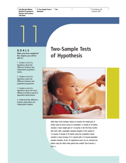
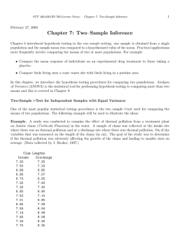
CHAPTER 11
Hypothesis Tests
Two
g
Sampl
n
i
v
l
o
Inv s or Proporti e
n
o
a
ns
e
M
GENDER STEREOTYPES AND
ASKING FOR DIRECTIONS
Many of us have heard the stereotypical observa-
this much lower just byВ chance. Section 11.6 of
tion that men absolutely refuse to stop and ask
this chapter will provideВ some guidance regarding
for directions, preferring instead to wander about
a statistical test with which you can compare
until they “find their own way.” Is this just a
these gender resultsВ and verify the conclusion for
stereotype, or is there really something to it?
yourself. ThereВ will be no need to stop at Section
When Lincoln Mercury was carrying out research
11.5 to askВ for directions.
prior to the design and introduction of its
Source: Jamie LaReau, “Lincoln Uses Gender Stereotypes to Sell
Navigation System,” Automotive News, May 30, 2005, p. 32.
in-vehicle navigational systems, the company
surveyed men and women with regard to their
driving characteristics and navigational habits.
According to the survey, 61% of the female
respondents said they would stop and ask for
directions once they figured out they were lost.
On the other hand, only 42% of the male respondents said they would stop and ask for directions
under the same circumstances. For purposes of our
discussion, we’ll assume that Lincoln Mercury surveyed 200 persons of each gender.
asking for men—a sample proportion of just 0.42
(84 out of 200) versus 0.61 (122 out of 200)—may
have occurred simply by chance variation? Actually,
if the population proportions were really the
same, there would be only a 0.0001 probability
ned way
of the direction-asking proportion for men being
-fashio
les the old
two samp
g
n
ri
a
p
Com
364
Reza Estakhrian/Stone/Getty Images
Is it possible that the lower rate of direction-
365
•
Select and use the appropriate hypothesis test in comparing the
means of two independent samples.
•
Test the difference between sample means when the samples
are not independent.
•
Test the difference between proportions for two independent
samples.
•
Determine whether two independent samples could have come
from populations having the same standard deviation.
LEARNING
OBJECTIVES
After reading this chapter,
you should be able to:
( )
INTRODUCTION
11.1
One of the most useful applications of business statistics involves comparing
two samples to examine whether a difference between them is (1) significant or
(2)В likely to have been due to chance. This lends itself quite well to the analysis
of data from experiments such as the following:
Comparing Samples
A local YMCA, in the early stages of telephone solicitation to raise funds for
expanding its gymnasium, is testing two appeals. Of 100 residents approached
with appeal A, 21% pledged a donation. Of 150 presented with appeal B, 28%
pledged a donation.
SOLUTION
Is B really a superior appeal, or could its advantage have been merely the result of
chance variation from one sample to the next? Using the techniques in this chapter, we can reach a conclusion on this and similar questions. The approach will
be very similar to that in Chapter 10, where we dealt with one sample statistic
(either }
x or p), its standard error, and the level of significance at which it differed
from its hypothesized value.
Sections 11.2–11.4 and 11.6 deal with the comparison of two means or two
proportions from independent samples. Independent samples are those for which
the selection process for one is not related to that for the other. For example, in
an experiment, independent samples occur when persons are randomly assigned
to the experimental and control groups. In these sections, a hypothesis-testing
procedure very similar to that in Chapter 10 will be followed. As before, either
one or two critical value(s) will be identified, and then a decision rule will be
applied to see if the calculated value of the test statistic falls into a rejection
region specified by the rule.
When comparing two independent samples, the null and alternative hypotheses
can be expressed in terms of either the population parameters (вђ®1 and вђ®2, or
вђІ1 and вђІ2) or the sampling distribution of the difference between the sample
statistics (}
x1 and }
x2, or p1 and p2). These approaches to describing the null and
alternative hypotheses are equivalent and are demonstrated in Table 11.1.
EXAMPLEEXAMPLEEXAMPLE
EXAMPLE
366
Part 4: Hypothesis Testing
TABLE 11.1
When comparing means from
independent samples, null and
alternative hypotheses can
be expressed in terms of the
population parameters (on the
left) or described by the mean
of the sampling distribution
of the difference between the
sample statistics (on the right).
This also applies to testing
two sample proportions. For
example, H0: вђІ1 5 вђІ2 is the
same as H0: вђ®(p 2p )5 0.
1
2
Null and Alternative
Hypotheses Expressed
in Terms of the
Population Means
Hypotheses Expressed in
Terms of the Sampling
Distribution of the Difference
Between the Sample Means
Two-tail test:
H 0:
вђ®1 5 вђ®2
H0:
вђ®( x} 2 x} ) 5 0
1
2
H1:
вђ®( x} 2 x} )
1
2
H0:
вђ®( x} 2 x} ) $ 0
H1:
вђ®( x} 2 x} ) , 0
H0:
вђ®( x} 2 x} ) # 0
1
2
H1:
вђ®( x} 2 x} ) . 0
1
2
or
H 1:
вђ®1
вђ®2
0
Left-tail test:
H 0:
вђ®1 $ вђ®2
or
H 1:
вђ®1 , вђ®2
1
1
2
2
Right-tail test:
H 0:
вђ®1 # вђ®2
or
H 1:
вђ®1 . вђ®2
Section 11.5 is concerned with the comparison of means for two dependent
samples. Samples are dependent when the selection process for one is related to
the selection process for the other. A typical example of dependent samples occurs
when we have before-and-after measures of the same individuals or objects. In
this case we are interested in only one variable: the difference between measurements for each person or object.
In this chapter, we present three different methods for comparing the means
of two independent samples: the pooled-variances t-test (Section 11.2), the
unequal-variances t-test (Section 11.3), and the z-test (Section 11.4). Figure 11.1
summarizes the procedure for selecting which test to use in comparing the sample
means.
As shown in Figure 11.1, an important factor in choosing between the
pooled-variances t-test and the unequal-variances t-test is whether we can assume the population standard deviations (and, hence, the variances) might be
equal. Section 11.7 provides a hypothesis-testing procedure by which we can actually test this possibility. However, for the time being, we will use a less rigorous
standard—that is, based on the sample standard deviations, whether it appears
that the population standard deviations might be equal.
( )
11.2
THE POOLED-VARIANCES t-TEST FOR COMPARING
THE MEANS OF TWO INDEPENDENT SAMPLES
Situations can arise where we’d like to examine whether the difference between
the means of two independent samples is large enough to warrant rejecting the
possibility that their population means are the same. In this type of setting, the
alternative conclusion is that the difference between the sample means is small
enough to have occurred by chance, and that the population means really could
be equal.
Chapter 11: Hypothesis Tests Involving Two Sample Means or Proportions
367
FIGURE 11.1
Selecting the test statistic for
hypothesis tests comparing the
means of two independent
samples.
Hypothesis test
m1 – m2
Are the population standard
deviations equal?
Does s1 = s2?
No
Yes
For any sample sizes
Compute the pooled estimate
of the common variance as
s2p =
(n1 – 1)s21 + (n2 – 1)s22
n1 + n2 – 2
and perform a pooled-variances
t-test where
t=
(x1 – x2) – (m1 – m 2)0
в€љ(
1
1
s2p –– + ––
n1
n2
)
Perform an unequal-variances
t-test where
t=
(x1 – x2) – (m1 – m 2)0
в€љ
s21
n1
+
s22
n2
and
[(s21 / n1) + (s22 / n2)]2
df =
(s21 / n1)2 (s22 / n2)2
+
n1 – 1
n2 – 1
df = n1 + n2 – 2
and (m1 – m2)0 is from H0
and (m1 – m2)0 is from H0
Test assumes samples are from
normal populations. When either
test can be applied to the same
data, the unequal-variances t-test is
preferable to the z-test—especially
when doing the test with computer
assistance.
Test assumes samples are from
normal populations with equal
standard deviations.
Section 11.2
See Note 1
Only if n1 and n2 both ≥ 30
A z-test approximation can be
performed where
z=
(x1 – x2) – (m1 – m 2)0
в€љ
s21 s22
+
n1 n2
with s21 and s22 as
s 21 and s 22 ,
estimates of
and (m1 – m2)0 is from H0
The central limit theorem
prevails and there are no
limitations on the population
distributions. This test may also
be more convenient for solutions
based on pocket calculators.
Section 11.4
See Note 3
Section 11.3
See Note 2
1. Section 11.7 describes a procedure for testing the null hypothesis that вђґ1 5 вђґ2. However,
when using a computer and statistical software, it may be more convenient to simply
bypass this assumption and apply the unequal-variances t-test described in Section 11.3.
2. This test involves a corrected df value that is smaller than if вђґ1 5 вђґ2 had been assumed.
When using a computer and statistical software, this test can be used routinely instead of
the other two tests shown here. The nature of the df expression makes hand calculations
somewhat cumbersome. The normality assumption becomes less important for larger
sample sizes.
3. When sample sizes are large (each n $ 30), the z-test is a useful alternative to the
unequal-variances t-test, and may be more convenient when hand calculations are
involved.
4. For each test, Computer Solutions within the chapter describe the Excel and Minitab
procedures for carrying out the test. Procedures based on data files and those based on
summary statistics are included.
368
Part 4: Hypothesis Testing
Our use of the t-test assumes that (1) the (unknown) population standard
deviations are equal, and (2) the populations are at least approximately normally
distributed. Because of the central limit theorem, the assumption of population
normality becomes less important for larger sample sizes. Although it is often
associated only with small-sample tests, the t distribution is appropriate when
the population standard deviations are unknown, regardless of how large or
small the samples happen to be.
The t-test used here is known as the pooled-variances t-test because it involves
the calculation of an estimated value for the variance that both populations are
assumed to share. This pooled estimate is shown in Figure 11.1 as s2p. The number
of degrees of freedom associated with the test will be df 5 n1 1 n2 2 2, and the
test statistic is calculated as follows:
Test statistic for comparing the means of two independent samples, вђґ1 and вђґ2
assumed to be equal:
x1 2 }
x2) 2 (вђ®1 2 вђ®2)0
(}
t 5 _____________________
wwwwww
1
1
s2p ___ 1 ___
n1 n2
ГЏ (
with
)
x1 and }
x2 5 means of samples 1 and 2
where }
(вђ®1 2 вђ®2)0 5 the hypothesized difference
between the population
means
n1 and n2 5 sizes of samples 1 and 2
s1 and s2 5 standard deviations of
samples 1 and 2
sp 5 pooled estimate of the
common standard deviation
(n1 2 1)s21 1 (n2 2 1)s22
s2p 5 _____________________
n1 1 n2 2 2
and
df 5 n1 1 n2 2 2
Confidence interval for вђ®1 2 вђ®2:
(}
x1 2 }
x2) 6 tвђЈy2
ГЏ (
wwwwww
1
1
2
sp ___ 1 ___
n1 n2
)
with
вђЈ 5 (1 2 confidence coefficient)
The numerator of the t-statistic includes (вђ®1 2 вђ®2)0, the hypothesized value
of the difference between the population means. The hypothesized difference is
generally zero in tests like those in this chapter. The term in the denominator of
the t-statistic is the estimated standard error of the difference between the sample
means. It is comparable to the standard error of the sampling distribution for the
sample mean discussed in Chapter 10. Also shown is the confidence interval for
the difference between the population means.
Chapter 11: Hypothesis Tests Involving Two Sample Means or Proportions
Pooled-Variances t-Test
Entrepreneurs developing an accounting review program for persons preparing
to take the Certified Public Accountant (CPA) examination are considering two
possible formats for conducting the review sessions. A random sample of 10 students are trained using format 1, and then their number of errors is recorded for
a prototype examination. Another random sample of 12 individuals are trained
according to format 2, and their errors are similarly recorded for the same examination. For the 10 students trained with format 1, the individual performances
are 11, 8, 8, 3, 7, 5, 9, 5, 1, and 3 errors. For the 12 students trained with format
2, the individual performances are 10, 11, 9, 7, 2, 11, 12, 3, 6, 7, 8, and 12 errors.
These data are in file CX11CPA.
SOLUTION
Since the study was not conducted with directionality in mind, the appropriate test will be two-tail. The null hypothesis is H0: вђ®1 5 вђ®2, and the alternative
hypothesis is H1: вђ®1
вђ®2. The null and alternative hypotheses may also be
expressed as follows:
•
Null hypothesis
H0:
•
вђ®(x}12x}2) 5 0
The two review formats are equally effective.
Alternative hypothesis
H1:
вђ®(x}12x}2)
0
The two review formats are not equally effective.
In comparing the performances of the two groups, the 0.10 level of significance
will be used. Based on these data, the 10 members of group 1 made an average
of 6.000 errors, with a sample standard deviation of 3.127. The 12 students
trained with format 2 made an average of 8.167 errors, with a standard deviation
of 3.326. The sample standard deviations do not appear to be very different,
and we will assume that the population standard deviations could be equal. (As
noted previously, this rather informal inference can be replaced by the separate
hypothesis test in Section 11.7.) In applying the pooled-variances t-test,
the pooled estimate of the common variance, s2p, and the test statistic, t, can
be calculated as
(10 2 1)(3.127)2 1 (12 2 1)(3.326)2
s2p 5 _________________________________ 5 10.484
10 1 12 2 2
and
(6.000 2 8.167) 2 0
t 5 ___________________ 5 21.563
wwwwwwww
1
1
10.484 ___ 1 ___
10
12
ГЏ
(
)
For the 0.10 level of significance, the critical values of the test statistic will be
t 5 21.725 and t 5 11.725. These are based on the number of degrees of
freedom, df 5 (n1 1 n2 2 2), or (10 1 12 2 2) 5 20, and the specification that
EXAMPLEEXAMPLEEXAMPLEEXAMPLEEXAMPLEEXAMPLEEXAMPLEEXAMPLEEXAMPLEEXA
EXAMPLE
369
370
Part 4: Hypothesis Testing
FIGURE 11.2
EXAMPLEEXAMPLEEXAMPLEEXAMPLEEXAMPLEEXAMPLEEXAMPLEEXAMPLE
In this two-tail pooled-variances
t-test, we are not able to reject
the null hypothesis that the
two accounting review formats
could be equally effective.
H0: m(x1 – x2) = 0
The two training formats are equally effective.
The two training formats are not equally effective.
H1: m(x1 – x2) ≠0
x1 and x2 are the mean numbers of errors for group 1 and group 2.
Reject H0
Do not reject H0
Reject H0
Area = 0.05
Area = 0.05
m(x1 – x2) = 0
t = –1.725
Test statistic:
t = –1.563
t = +1.725
the two tail areas must add up to 0.10. The decision rule is to reject the null
hypothesis (i.e., conclude that the population means are not equal for the two
review formats) if the calculated test statistic is either less than t 5 21.725 or
greater than t 5 11.725.
As Figure 11.2 shows, the calculated test statistic, t 5 21.563, falls into the
nonrejection region of the test. At the 0.10 level, we must conclude that the review
formats are equally effective in training individuals for the CPA examination. For
this level of significance, the observed difference between the groups’ mean errors
is judged to have been due to chance.
Based on the sample data, we will also determine the 90% confidence interval
for (вђ®1 2 вђ®2). For df 5 20 and вђЈ 5 0.10, this is
(}
x1 2 }
x2) 6 tвђЈy2
ГЏ(
wwwww
1
2 1
)
sp ___ 1 ___ 5 (6.000 2 8.167) 6 1.725
n1 n2
ГЏ10.484( 10 1 12 )
wwwwwwww
1
1
___
___
5 22.167 6 2.392, or from 24.559 to 10.225
The hypothesized difference (zero) is contained within the 90% confidence
interval, so we are 90% confident the population means could be the same. As
discussed in Chapter 10, a nondirectional test at the вђЈ level of significance and
a 100(1 2 вђЈ)% confidence interval will lead to the same conclusion. Computer
Solutions 11.1 shows Excel and Minitab procedures for the pooled-variances
t-test.
Chapter 11: Hypothesis Tests Involving Two Sample Means or Proportions
371
COMPUTER 11.1 SOLUTIONS
Pooled-Variances t-Test for (вђ®1 2 вђ®2), Population Variances Unknown but
Assumed Equal
These procedures show how to use the pooled-variances t-test to compare the means of two independent
samples. The population variances are unknown, but assumed to be equal.
EXCEL
Excel pooled-variances t-test for (вђ®1 2 вђ®2), based on raw data
1. For the sample data (Excel file CX11CPA) on which Figure 11.2 is based, with the label and 10 data values for
format 1 in column A, and the label and 12 data values for format 2 in column B: From the Data ribbon, click Data
Analysis. Click t-Test: Two-Sample Assuming Equal Variances. Click OK.
2. Enter A1:A11 into the Variable 1 Range box and B1:B13 into the Variable 2 Range box. Enter 0 into the
Hypothesized Mean Difference box. Click to select Labels. Specify the significance level for the test by entering
0.10 into the Alpha box. Select Output Range and enter D1 into the box. Click OK. The results will be as shown
above. This is a two-tail test, so we refer to the 0.134 p-value. (Excel doesn’t ask whether our test is one-tail or
two-tail, but it provides critical values and p-values for both.)
3. To obtain a confidence interval for (вђ®1 2 вђ®2), it will be necessary to refer to the procedure described below. It is
based on summary statistics for the samples.
Excel Unstacking Note: When this analysis is based on raw data, Excel requires that the two samples be in two
distinctly separate fields (e.g., two separate columns). If the data are in one column and the subscripts identifying group
membership are in another column, it will be necessary to “unstack” the data. For example, if the data were in column
A and theВ subscripts (1 and 2, to denote prep formats 1 and 2) were in column B, and each column had a label at the
top: Click and drag to select the numbers and labels in columns A and B. From the Data ribbon, click Sort. In the Sort
by box, select the category variable in column B (i.e., Format). Click OK. The data for sample 1 will now be listed directly
above the data for sample 2—from here, we need only select each grouping of data (e.g., scores) and either move
or copy it toВ its own column. The result will be one column for the scores of group 1 and an adjacent column for the
scores of group 2.
Excel pooled-variances t-test and confidence interval for (вђ®1 2 вђ®2), based on summary statistics
1. Using the summary statistics associated with CX11CPA: Open the TEST STATISTICS workbook.
2. Using the arrows at the bottom left, select the t-Test_2 Means (Eq-Var) worksheet.
(continued )
372
Part 4: Hypothesis Testing
3. Enter the sample means, variances, and sizes into the appropriate cells. Enter the hypothesized difference (0, in this
case) and the desired alpha level for the test. The calculated t-statistic and a two-tail p-value will be shown at the right.
4. To obtain a confidence interval for (␮1 2 ␮2), follow steps 1–3, but open the ESTIMATORS workbook and select the
t-Estimate_2 Means (Eq-Var) worksheet. Enter the desired confidence level as a decimal fraction (e.g., 0.90).
Note: As an alternative, you can use Excel worksheet template TMT2POOL. It simultaneously conducts the test and reports
a confidence interval. The steps are described within the template.
MINITAB
Minitab pooled-variances t-test and confidence interval for (вђ®1 2 вђ®2), based on raw data
1. For example, using the data (Minitab file CX11CPA) on which Figure 11.2 is based, with the data values for format 1 in
column C1 and the data values for format 2 in column C2: Click Stat. Select Basic Statistics. Click 2-Sample t.
2. Select Samples in different columns. Enter C1 into the First box and C2 into the Second box. Click to select
Assume equal variances. (Note: If all the data had been in a single column [i.e., “stacked”], it would have been
necessary to select the Samples in one column option, then to specify the column containing the data and the
column containing the subscripts identifying group membership.)
3. Click Options. Enter the desired confidence level as a percentage (e.g., 90.0) into the Confidence Level box. Enter
the hypothesized difference (0) into the Test difference box. Within the Alternative box, select not equal. Click
OK. Click OK.
Minitab pooled-variances t-test and confidence interval for (вђ®1 2 вђ®2), based on summary data
Follow steps 1 through 3 above, but select Summarized data in step 2 and insert the appropriate summary statistics
into the Sample size, Mean, and Standard deviation boxes for each sample.
ERCISES
X
E
11.1 “When comparing two sample means, the t-test
should be used only when the sample sizes are less than
30.” Comment.
11.2 An educator is considering two different videotapes for use in a half-day session designed to introduce
students to the basics of economics. Students have been
randomly assigned to two groups, and they all take the
same written examination after viewing the videotape.
The scores are summarized here. Assuming normal populations with equal standard deviations, does it appear
that the two videotapes could be equally effective? What
is the most accurate statement that could be made about
the p-value for the test?
} 5 77.1
Videotape 1: x
1
} 5 80.0
Videotape 2: x
2
s1 5 7.8
n1 5 25
s2 5 8.1
n2 5 25
11.3 Using independent random samples, a researcher
is comparing the number of hours of television viewed
last week for high school seniors versus sophomores. The
results are shown here. Assuming normal populations
Chapter 11: Hypothesis Tests Involving Two Sample Means or Proportions
with equal standard deviations, does it appear that the
average number of television hours per week could
be equal for these two populations? What is the most
accurate statement that could be made about the p-value
for the test?
Seniors:
Sophomores:
} 5 3.9 hours s 5 1.2 hours n 5 32
x
1
1
1
} 5 3.5 hours s 5 1.4 hours n 5 30
x
2
2
2
11.4 An ambulance service located at the edge of town is
responsible for serving a large office building in the downtown area. Testing different routes for getting from the
ambulance station to the office building, a driver finds that
five trips using route A take an average of 5.9 minutes,
with a standard deviation of 1.4 minutes; six trips using
route B take an average of 4.2 minutes, with a standard
deviation of 1.8 minutes. Assuming normal populations
with equal standard deviations, and using the 0.10 level,
is there a significant difference between theВ two routes?
Construct and interpret the 90% confidence interval for
the difference between the population means.
11.5 A maintenance supervisor is comparing the standard
version of an instructional booklet with one that has been
claimed to be superior. An experiment is conducted in
which 26 technicians are divided into two groups,
provided with one of the booklets, then given a test a
week later. For the 13 using the standard version, the
average exam score was 72.0, with a standard deviation
of 9.3. For the 13 given the new version, the average
score was 80.2, with a standard deviation of 10.1. Assuming
normal populations with equal standard deviations, and
using the 0.05 level of significance, does the new booklet
appear to be better than the standard version?
11.6 A sample of 40 investment customers serviced by
an account manager are found to have had an average
of $23,000 in transactions during the past year, with a
standard deviation of $8500. A sample of 30 customers
serviced by another account manager averaged $28,000
in transactions, with a standard deviation of $11,000.
Assuming the population standard deviations are equal,
use the 0.05 level of significance in testing whether the
population means could be equal for customers serviced
by the two account managers. Using the appropriate
statistical table, what is the most accurate statement we
can make about the p-value for this test? Construct and
interpret the 95% confidence interval for the difference
between the population means.
11.7 Comparing dexterity-test scores of workers on the
day shift versus those on the night shift, the production
manager of a large electronics plant finds that a sample
of 37 workers from the day shift have an average score of
73.1, with a standard deviation of 12.3. For 42 workers
from the night shift, the average score was 77.3, with
a standard deviation of 8.4. Assuming the population
standard deviations are equal, use the 0.05 level of
significance in comparing the average scores for the two
373
shifts. Using the appropriate statistical table, what is
theВ most accurate statement we can make about the
p-value for this test? Construct and interpret the 95%
confidence interval for the difference between the
population means.
11.8 Sheila Smith, the manager of a large resort’s main
hotel, has been receiving complaints from some guests
that they are not being provided with prompt service
upon approaching the front desk. In particular, she is
concerned that desk staff might be providing female
guests with less prompt service than their male counterparts. In observing a sample of 34 male guests, she finds
it takes an average of 15.2 seconds, with a standard
deviation of 5.9 seconds, for them to be greeted after
their arrival at the front desk. For a sample of 39 female
guests, the mean and standard deviation are 17.4 seconds
and 6.4 seconds, respectively. Assuming the population
standard deviations to be equal, use the 0.05 level of
significance in examining whether the populationВ mean
time for serving female guests might actually be no
greater than that for serving male guests. Using the
appropriate statistical table, what is the most accurate
statement we can make about the p-value for theВ test?
11.9 Media observers have been examining the numberВ of minutes devoted to business and financial news
duringВ the half-hour evening news broadcasts of two
local television channels. For each channel, they have
randomly selected 10 weekday broadcasts and observed
the number of minutes spent on business andВ financial
news during that broadcast. The times measured in these
independent samples are shown here.В Assuming normal
populations with equal standard deviations, use the 0.10
level of significance inВ testing whether the population
means might actually be the same. Using the appropriate
statistical table, what is the most accurate statement we
can make aboutВ the p-value for the test? Construct and
interpretВ the 90% confidence interval for the difference
between the population means.
Channel 2: 3.8 2.7 4.9 3.4 3.7 4.5 4.2 2.8 3.5 4.6 minutes
Channel 4: 3.6 4.0 4.5 5.2 4.8 4.3 5.7 3.5 3.7 5.8 minutes
11.10 In a test of the effectiveness of a new battery design,
16 battery-powered music boxes are randomly provided
with either the old design or the new version. Hours of
playing time before battery failure were as follows:
8 boxes,
new battery type:
3.3, 6.4, 3.9, 5.4,
5.1, 4.6, 4.9, 7.2 hrs
8 boxes,
old battery type:
4.2, 2.9, 4.5, 4.9,
5.0, 5.1, 3.2, 4.0 hrs
Assuming normal populations with equal standard
deviations, use the 0.05 level to determine whether the
new battery could be better than the old design. Using
the appropriate statistical table, what is the most accurate
statement we can make about the p-value for this test?
374
Part 4: Hypothesis Testing
11.11 A nutritionist has noticed a FoodFarm ad stating the company’s peanut butter contains less fat than
that produced by a major competitor. She purchases
11 8-ounce jars of each brand and measures the fat
content of each. The 11 FoodFarm jars had an average of 31.3В grams of fat, with a standard deviation of
2.1 grams. The 11 jars from the other company had an
average of 33.2 grams of fat, with a standard deviation
of 1.8 grams. Assuming normal populations with equal
standard deviations, use the 0.05 level of significance in
examining whether FoodFarm’s ad claim could be valid.
What is the most accurate statement that could be made
about the p-value for this test?
0.05 level, was the mean return speed for the flattened bat
significantly greater than for the regulation bat? Identify
and interpret the p-value for the test. Source: Andy Gardiner,
( DATA SET ) Note: Exercises 11.12–11.17 require a
computer and statistical software.
Source: ”Primates on Facebook,” economist.com, February 26, 2009.
11.12 A study published in the Archives of Internal
Medicine examined the prevalence of so-called “difficult”
patients who ask for unneeded prescriptions, unnecessarily
complain, or otherwise cause extraordinary frustrations
for their medical provider. Researchers found the mean
age of doctors having the greatest problems with difficult
patients was 41, while the mean age of doctors having the
least problems with difficult patients was 46. Assume that
data file XR11012 contains the ages for doctors in each of
these patient-difficulty samples. In a suitable one-tail test
at the 0.01 level, was the mean age for doctors having the
greatest problems with difficult patients significantly less
than that for those having the least problems with difficult
patients? Identify and interpret the p-value for the test.
Source: Rita Rubin, “�Difficult Patients Can Test Doctors’ Patience,“ USA
Today, February 24, 2009, p. 5D.
11.13 It has been claimed that flattening (“rolling”) the
barrel of a graphite baseball bat can stretch the fibers
and result in a pitched baseball being returned faster than
with a regulation bat. This was a controversial topic during the 2009 baseball College World Series. Assume that
data file XR11013 describes the results of a controlled test
measuring the return speeds of balls pitched to a flattened
bat and a regulation bat, respectively. Based on these
sample results, and using a suitable one-tail test at the
( )
11.3
“NCAA on Guard for �Rolled’ Bats,” USA Today, June 17, 2009, p. 8C.
11.14 Comparing the number of Facebook “friends” for
men and women, observers have speculated about whether
the mean number of friends could be the same for each
group. Assume that data file XR11014 lists the number of
Facebook friends for independent samples of male and
female Facebook users. Based on the results of a two-tail
test at the 0.05 level, comment on whether the difference
between the sample means could have simply occurred by
chance. Identify and interpret the p-value for the test.
11.15 Using the sample results in Exercise 11.14, construct and interpret the 95% confidence interval for the
difference between the population means. Is the hypothesized difference (0.00) within the interval? Given the
presence or absence of the 0.00 value within the interval,
is this consistent with the findings of the hypothesis test
conducted in Exercise 11.14?
11.16 An engineer has measured the hardness scores
for a sample of conveyor-belt support bearings that
have been hardened by two different methods. The first
method is used by her company, and the second method
is known to be used by a number of other companies
in the industry. With the resulting data in file XR11016,
use the 0.05 level of significance in comparing the mean
hardness scores of the two samples, and comment on the
possibility that the difference between the sample means
could have occurred by chance. Identify and interpret the
p-value for the test.
11.17 Using the sample results in Exercise 11.16, construct and interpret the 95% confidence interval for the
difference between the population means. Is the hypothesized difference (0.00) within the interval? Given the
presence or absence of the 0.00 value within the interval,
is this consistent with the findings of the hypothesis test
conducted in Exercise 11.16?
THE UNEQUAL-VARIANCES t-TEST FOR COMPARING
THE MEANS OF TWO INDEPENDENT SAMPLES
When the population standard deviations are unknown and are not assumed to
be equal, pooling the sample standard deviations into a single estimate of their
common population value is no longer applicable. As a result, s1 and s2 must be
used to estimate their respective population standard deviations, вђґ1 and вђґ2. The
test assumes the populations to be at least approximately normally distributed,
an assumption that becomes less important for larger sample sizes.
In the unequal-variances t-test, the t-statistic expression is straightforward, but
the df formula is a little more complex—it is a correction formula that provides a
Chapter 11: Hypothesis Tests Involving Two Sample Means or Proportions
375
df value that is smaller than its counterpart in the preceding section. For accuracy,
it’s best to maintain a lot of decimal places if you are computing df with a pocket calculator. If we are using the computer and statistical software, the unequal-variances
t-test presents no computational difficulties, and is the preferred method for
comparing the means of two independent samples, regardless of the sample sizes.
The test statistic, df, and confidence interval expressions for this test are shown here:
Unequal-variances t-test for comparing the means of two independent samples,
вђґ1 and вђґ2 unknown and not assumed to be equal:
x1 2 }
x2) 2 (вђ®1 2 вђ®2)0
(}
t 5 _____________________
wwww
s22
s21
___
1 ___
n1 n2
ГЏ
with
where }
x1 and }
x2 5 means of samples 1 and 2
(вђ®1 2 вђ®2)0 5 hypothesized difference
between the population
means
n1 and n2 5 sizes of samples 1 and 2
s1 and s2 5 standard deviations of
samples 1 and 2
f ( s21yn1 ) 1 ( s22yn2 ) g2
df 5 __________________
( s21yn1 )2 _______
( s22yn2 )2
_______
1
n1 2 1
n2 2 1
Confidence interval for вђ®1 2 вђ®2:
with
} 2}
(x
x2) 6 tвђЈ/2
1
ГЏ
wwww
s2
s2
1
2
___
1 ___
n1
n2
вђЈ 5 (1 2 confidence coefficient)
Unequal-Variances t-Test
The makers of Graphlex, a graphite additive for engine oil, have conducted an
experimental study to determine the effectiveness of their product in improving
the fuel efficiency of automobiles. In cooperation with the Metropolitan Cab
Company, they’ve randomly divided the company’s cabs into two groups of equal
size. Graphlex was added to the engine oil of the 45 cabs in the experimental
group, while the 45 cabs in the control group continued to operate with the
usual lubricant. Drivers were not informed of the experiment. After 1 month,
fuel efficiency records were examined. For the 45 cabs using Graphlex, the
average cab achieved 18.94 miles per gallon (mpg), with a standard deviation
of 3.90 mpg. For the 45 cabs not using Graphlex, the average mpg was 17.51,
with a standard deviation of 2.87 mpg. The underlying data are in file CX11MPG.
Graphlex is preparing a national advertising campaign to promote its ability to
improve fuel efficiency.
EXAMPLEEXAMPLEEXAMPLEEXAM
EXAMPLE
376
Part 4: Hypothesis Testing
FIGURE 11.3
The makers of Graphlex claim
their graphite oil additive
improves the fuel efficiency of
automobiles. InВ this right-tail
unequal-variances test at the
0.05 level, the results indicate
they may be correct.
H0: m(x1 – x2) ≤ 0
mpg with Graphlex is no higher than for ordinary oil.
Graphlex improves fuel economy.
H1: m(x1 – x2) > 0
x1 and x2 are mpg averages for cabs with and without Graphlex.
Do not reject H0
Reject H0
Area = 0.05
m(x1 – x2) = 0
LEEXAMPLEEXAMPLEEXAMPLEEXAMPLEEXAMPLEEXAMPLE
t = +1.664
Test statistic:
t = +1.98
SOLUTION
The results will be evaluated at the 0.05 level of significance. Since the purpose of
the study was to determine whether cabs using Graphlex (group 1) get better fuel
economy than cabs without it (group 2), the null and alternative hypotheses are
H0: вђ®1 # вђ®2, and H1: вђ®1 . вђ®2. Expressed in terms of the sampling distribution
of the difference between sample means, the null and alternative hypotheses can
be stated as follows:
•
•
Null hypothesis
H0: вђ®(}x12}x2) # 0
mpg with Graphlex is no higher than
with conventional oil.
Alternative hypothesis
H1: вђ®(}x12}x2) . 0
mpg with Graphlex is higher.
For these data, the values for the test statistic (t) and the number of degrees of
freedom (df ) are calculated as
x1 2 }
x2) 2 (вђ®1 2 вђ®2)0
(}
(18.94 2 17.51) 2 0
t 5 _____________________ 5 ___________________ 5 1.98
2
2
wwww
wwwwwww
s1
s2
3.902 _____
2.872
_____
___
1
1 ___
n1
n2
45
45
and
[(3.902Y45) 1 (2.872Y45)]2
3 ( s21Yn1 ) 1 ( s22Yn2 ) 42
df 5 _________________ 5 ________________________ 5 80.85, rounded to 81
(3.902Y45)2
(2.872Y45)2
( s21Yn1 )2 _______
( s22Yn2 )2 ___________
___________
_______
1
1
45 2 1
45 2 1
n1 2 1
n2 2 1
ГЏ
ГЏ
For the 0.05 level of significance, df 5 81, and a right-tail test, the critical
value of the test statistic is t 5 11.664. The decision rule is, “Reject H0 if the
calculated test statistic is greater than t 5 11.664, otherwise do not reject.” As
Figure 11.3 shows, the calculated test statistic exceeds the critical value, the null
hypothesis is rejected, and we conclude that Graphlex really works.
Chapter 11: Hypothesis Tests Involving Two Sample Means or Proportions
377
NOTE
As we saw in Chapter 10, different levels of significance can lead to different
conclusions. For example, at the 0.01 level (critical t 5 12.373), the null hypothesis would not have been rejected. While the Graphlex Company would likely
stress the additive’s effectiveness by relying on the 0.05 level of significance, the
manufacturer of a competing brand would tend to prefer a more demanding test
(e.g., вђЈ 5 0.01) in order to boast that Graphlex has no effect.
You may have noticed that the degrees of freedom value for this test, df 5
81, was near the upper part of the df range of the t distribution table. Should you
encounter a test in which df happens to be over 100, just use the “infinity” row of
the table to determine the critical value(s) of the test statistic. This row represents the
normal distribution, toward which the t distribution converges as df becomes larger.
Based on the sample data, we will also determine the 90% confidence interval
for (вђ®1 2 вђ®2). For df 5 81 and вђЈ 5 0.10, this will be
x1 2 }
x2) 6 tвђЈy2
(}
ГЏ
wwww
s2
s2
ГЏ
1
2
___
1 ___ 5 (18.94 2 17.51) 6 1.664
n1
n2
wwwwwww
3.902
2.872
_____ 1 _____
45
45
5 1.43 6 1.20, or from 0.23 to 2.63
Computer Solutions 11.2 shows Excel and Minitab procedures for the
unequal-variances t-test.
COMPUTER 11.2 SOLUTIONS
Unequal-Variances t-Test for (вђ®1 2 вђ®2), Population Variances
Unknown and Not Equal
These procedures show how to use the unequal-variances t-test to compare the means of two independent
samples. The population variances are unknown and not assumed to be equal.
EXCEL
Excel unequal-variances t-test for (вђ®1 2 вђ®2), based on raw data
1. For the sample data (Excel file CX11MPG) on which Figure 11.3 is based, with the label and 45 mpg values for the
Graphlex cabs in column A, and the label and 45 data values for the standard cabs in column B: From the Data ribbon,
click Data Analysis. Click t-Test: Two-Sample Assuming Unequal Variances. Click OK.
(continued )
378
Part 4: Hypothesis Testing
2. Enter A1:A46 into the Variable 1 Range box and B1:B46 into the Variable 2 Range box. Enter 0 into the
Hypothesized Mean Difference box. Click to select Labels. Specify the significance level by entering 0.05 into
the Alpha box. Select Output Range and enter D1 into the box. Click OK. This is a one-tail test, so we refer to
the 0.026 p-value.
3. To obtain a confidence interval for (вђ®1 2 вђ®2), it will be necessary to refer to the procedure described next. It is based
on summary statistics for the samples.
Note: For an analysis based on raw data, Excel requires the two samples to be in two distinctly separate fields (e.g., two
separate columns). If the data are in one column and the subscripts identifying group membership are in another column,
see the Excel Unstacking Note in Computer Solutions 11.1.
Excel unequal-variances t-test and confidence interval for (вђ®1 2 вђ®2), based on summary statistics
1. Using the summary statistics associated with CX11MPG (the test is summarized in Figure 11.3): Open the TEST
STATISTICS workbook.
2. Using the arrows at the bottom left, select the t-Test_2 Means (Uneq-Var) worksheet.
3. Enter the sample means, variances, and sizes into the appropriate cells. Enter the hypothesized difference (0, in
this case) and the desired alpha level for the test. The calculated t-statistic and a one-tail p-value will be shown
at the right.
4. To get a confidence interval for (␮1 2 ␮2), follow steps 1–3, above, but open the ESTIMATORS workbook and select
the t-Estimate_2 Means (Uneq-Var) worksheet. Enter the desired confidence level as a decimal fraction (e.g.,В 0.90).
Note: As an alternative, you can use Excel worksheet template TMT2UNEQ. It simultaneously conducts the test and
reports a confidence interval. The steps are described within the template.
MINITAB
Minitab unequal-variances t-test and confidence interval for (вђ®1 2 вђ®2), based on raw data
1. For example, using the data (Minitab file CX11MPG) on which Figure 11.3 is based, with the data values for the
Graphlex cabs in column C1 and the data values for the standard cabs in column C2: Click Stat. Select Basic
Statistics. Click 2-Sample t.
2. Select Samples in different columns. Enter C1 into the First box and C2 into the Second box. Do NOT select the
“Assume equal variances” option. (Note: If all the data had been in a single column [i.e., “stacked”], it would have
been necessary to select the Samples in one column option, then to specify the column containing the data and
the column containing the subscripts identifying group membership.)
3. Click Options. Enter the desired confidence level as a percentage (e.g., 90.0) into the Confidence Level box.
Enter the hypothesized difference (0) into the Test difference box. Within the Alternative box, select greater
than. Click OK. Click OK.
Minitab unequal-variances t-test and confidence interval for (вђ®1 2 вђ®2), based on summary data
Follow steps 1 through 3 above, but select Summarized data in step 2 and insert the appropriate summary statistics
into the Sample size, Mean, and Standard deviation boxes for each sample.
Chapter 11: Hypothesis Tests Involving Two Sample Means or Proportions
379
ERCISES
X
E
11.18 In two independent samples from populations that
are normally distributed, 2
x1 5 35.0, s1 5 5.8, n1 5 12
and 2
x2 5 42.5, s2 5 9.3, n2 5 14. Using the 0.05 level of
significance, test H0: вђ®1 5 вђ®2 versus H1: вђ®1 ? вђ®2.
11.19 In two independent samples, 2
x1 5 165.0, s1 5
21.5, n1 5 40 and 2
x2 5 172.9, s2 5 31.3, n2 5 32.
Using the 0.10 level of significance, test H0: вђ®1 $ вђ®2
versus H1: вђ®1 , вђ®2.
11.20 In two independent samples, 2
x1 5 125.0, s1 5
21.5, n1 5 40, and 2
x2 5 116.4, s2 5 10.8, n2 5 35.
Using the 0.025 level of significance, test H0: вђ®1 # вђ®2
versus H1: вђ®1 . вђ®2.
11.21 Fred and Martina, senior agents at an airline secu-
rity checkpoint, carry out advanced screening procedures
for hundreds of randomly selected passengers per day. For
a random sample of 30 passengers recently processed by
Fred, the mean processing time was 124.5 seconds, with a
standard deviation of 20.4 seconds. For a random sample
of 36 passengers recently processed by Martina, the corresponding mean and standard deviation were 133.0 seconds and 38.7 seconds, respectively. Using the 0.05 level
of significance, can we conclude that the population mean
processing times for Fred and Martina could be the same?
Using the appropriate statistical table, what is the most
accurate statement we can make about the p-value for
the test? Construct and interpret the 95% confidence
interval for the difference between the population
means.
11.22 A tire company is considering switching to a new
type of adhesive designed to improve tire reliability in
high-temperature and overload conditions. In laboratory “torture” tests with temperatures and loads 90%
higher than the maximum normally encountered in the
field, 15В tires constructed with the new adhesive run
an average of 65 miles before failure, with a standard
deviation of 14 miles. For 18 tires constructed with the
conventional adhesive, the mean mileage before failure
was 53 miles, with a standard deviation of 22 miles.
Assuming normal populations and using the 0.05 level
ofВ significance, can we conclude that the new adhesive
is superior to the old under such test conditions? What
is the most accurate statement that could be made about
the p-value for this test?
11.23 The credit manager for Braxton’s Department
Store, in examining the accounts for various types of customers served by the establishment, has noticed that the
mean outstanding balance for a sample of 20 customers
from the local ZIP code is $375, with a standard deviation of $75. For a sample of 25 customers from a nearby
ZIP code, the mean and standard deviation were $425
and $143, respectively. Assuming normal populations
and using the 0.05 level of significance, examine whether
credit customers from the two ZIP codes might have the
same mean outstanding balance. What is the most
accurate statement that could be made about the p-value
for this test? Construct and interpret the 95% confidence
interval for the difference between the population means.
Is the hypothesized difference (0.00) within the interval?
Given the presence or absence of the 0.00 value within
the interval, is this consistent with the findings of the
hypothesis test?
11.24 Safety engineers at a manufacturing plant are
evaluating two brands of 50-ampere electrical fuses
for possible purchase and use in the plant. One of the
performance characteristics they are considering is how
long the fuse will carry 50 amperes before it blows. In a
sample of 35 fuses from the Shockley Fuse Company, the
mean timeВ was found to be 240 milliseconds, with a standard deviation of 50 milliseconds. In comparable tests of
a sample of 30 fuses from the Fusemaster Corporation,
theВ mean time was 221 milliseconds, with a standard
deviation of 28 milliseconds. Using the 0.10 level of
significance, examine whether the population mean times
for fuses from the two companies might be the same.
What is the most accurate statement that could be made
about the p-value for this test? Construct and interpret
the 90% confidence interval for the difference between
the population means. Is the hypothesized difference
(0.00) within the interval? Given the presence or absence
of the 0.00 value within the interval, is this consistent
with the findings of the hypothesis test?
11.25 According to a national Gallup poll, men visit the
doctor’s office an average of 3.8 times per year, while
women visit an average of 5.8 times per year. In a similar
poll conducted in a Midwest county, a sample of 50 men
visited the doctor an average of 2.2 times in the past
year, with a standard deviation of 0.6 visits. For a sample
of 40 women from the same county, the mean and standard deviation were 3.9 and 0.9, respectively. In a twotail test at the 0.05 level, test whether the observed difference between x}1 and x}2 is significantly different from
the (3.8 2 5.8)5 22.0 visits per year that was found
for the nation as a whole. Construct and interpret the
95% confidence interval for (вђ®1 2 вђ®2) for the county. Is
the hypothesized difference (22.0) within the interval?
Given the presence or absence of the 22.0 value within
the interval, is this consistent with the findings of the
hypothesis test? Source: Cindy Hall and Marcy E. Mullins, “Doctors
See Women More Often,” USA Today, May 2, 2000, p. 7D.
380
Part 4: Hypothesis Testing
11.26 One of the measures of the effectiveness of a stimulus
is how much the viewer’s pulse rate increases on exposure
to it. In testing a lively new music theme for its television
commercials, an advertising agency shows ads with the new
music to a sample of 25 viewers. Their mean pulse rate
increase is 20.5 beats per minute, with a standard deviation
of 7.4. For a comparable sample of 25В viewers seeing the
same ads with the previous music theme, the mean pulse
rate increase is 16.4 beats per minute, with a standard deviation of 4.9. Assuming normal populations and using the
0.025 level of significance, can we conclude that the new
music theme is better than the old in terms of increasing the
pulse rate of viewers? What is the most accurate statement
that could be made about the p-value for this test?
( DATA SET ) Note:
Exercises 11.27–11.30 require a
computer and statistical software.
11.27 According to a Yankelovich poll, women spend
anВ average of 19.1 hours shopping during the month of
December, compared to 12.7 hours for men. Assuming
that file XR11027 contains the survey data underlying
these results, use the 0.01 level in examining whetherВ the
sample mean for women is significantly higher than that
for men. Identify and interpret the p-value for the test.
Source: Anne R. Carey and Gary Visgaitis, “�Tis the Season, Health,” USA
Today 1999 Snapshot Calendar, December 8.
11.28 When companies are designing a new product, one
of the steps typically taken is to see how potential buyers
react to a picture or prototype of the proposed product. The
product-development team for a notebook computer company has shown picture A to a large sample of potential
buyers and picture B to another, asking each person to indicate what they “would expect to pay” for such a product.
The data resulting from the two pictures are provided in
( )
11.4
file XR11028. Using the 0.05 level of significance, determine
whether the prototypes might not really differ in terms of
the price that potential buyers would expect to pay. Identify
and interpret the p-value for the test. Construct and interpret the 95% confidence interval for the difference between
the population means. Is the hypothesized difference (0.00)
within the interval? Given the presence or absence of the
0.00 value within the interval, is this consistent with the
findings of the hypothesis test?
11.29 It has been reported that the average visitor from
Japan spent $3120 during a trip to the United States, while
the average for a visitor from the United Kingdom was
$2654. Assuming that file XR11029 contains the survey
data underlying these results, use the 0.05 level inВ examining whether the sample mean for Japanese visitors is
significantly higher than that for visitors from the United
Kingdom. Identify and interpret the p-value for the test.
Source: The World Almanac and Book of Facts 2009, p. 127.
11.30 During May 2009, visitors to usatoday.com spent
an average of 12.2 minutes per visit, compared to 11.0
minutes for visitors to washingtonpost.com. Assuming
that file XR11030 contains the sample data underlying
these results, use the 0.01 level of significance in examining whether the population mean visiting times for
the two sites might really be the same. Identify and
interpret the p-value for the test. Construct and interpret the 99% confidence interval for the difference
between the population means. Is the hypothesized
difference (0.00) within the interval? Given the presence or absence of the 0.00 value within the interval, is
this consistent with the findings of the hypothesis test?
Source: Jennifer Saba, “Average Time Spent on Top 30 Newspaper Web
Sites Declines,” editorandpublisher.com, June 22, 2009.
THE z-TEST FOR COMPARING THE MEANS
OF TWO INDEPENDENT SAMPLES
The z-test approximation is included in Figure 11.1 and presented here as an
alternative to the unequal-variances t-test whenever both n1 and n2 are $30.
Besides requiring no assumptions about the shape of the population distributions, it offers the advantages of slightly greater simplicity and avoidance of the
cumbersome df correction formula used in the unequal-variances t-test; thus, it
can be useful to those who are not relying on a computer and statistical software. This test has been popular for many years as a method for comparing the
means of two large, independent samples when вђґ1 and вђґ2 are unknown, and of
two independent samples of any size when вђґ1 and вђґ2 are known and the two
populations are normally distributed. Like the unequal-variances t-test, the z-test
approximation does not assume the population standard deviations are equal,
and s1 and s2 are used to estimate their respective population standard deviations, вђґ1 and вђґ2.
Chapter 11: Hypothesis Tests Involving Two Sample Means or Proportions
381
z-test approximation for comparing the means of two independent samples, вђґ1
and вђґ2 unknown, and each n Х† 30:
} 2x
} ) 2 (вђ® 2 вђ® )
(x
1
2
1
2 0
} and x
} 5 means of samples 1 and 2
where x
z 5 _____________________
1
2
wwww
s22
s21
(вђ®
2
вђ®
)
5 hypothesized difference
1
2
0
___ П© ___
between the population means
n1 n2
n1 and n2 5 sizes of samples 1 and 2
s1 and s2 5 standard deviations of
samples 1 and 2
Confidence interval for вђ®1 2 вђ®2:
wwww
s22
s21
} 2x
} )6z
___
___
(x
1
1
2
вђЈy2 n
n2
1
with
вђЈ 5 (1 2 confidence coefficient)
ГЏ
ГЏ
z-Test
A university’s placement center has collected data comparing the starting salaries
of graduating students with surnames beginning with the letters A through M
with those whose surnames begin with N through Z. For a sample of 30 students
in the A–M category, the average starting salary was $37,233.33, with a standard
deviation of $3475.54. For a sample of 36 students with surnames beginning
with N–Z, the average starting salary was $35,855.81, with a standard deviation
of $2580.02. The underlying data are in file CX11GRAD.
SOLUTION
For this study, the null hypothesis is that there is no difference between the population means, or H0: вђ®1 5 вђ®2. Because the intent of the test is nondirectional, the
null hypothesis can be rejected by an extreme difference in either direction, and
the alternative hypothesis is H1: ␮1 ? ␮2. For testing the null hypothesis, we’ll use
the 0.02 level of significance. As described in Table 11.1, the null and alternative
hypotheses can also be stated as follows:
•
Null hypothesis
H0: вђ®(2x 22x ) 5 0
1
•
2
Alternative hypothesis
H1: вђ®(2x 22x ) Гћ 0
1
2
The starting salaries are the same
for both populations.
The starting salaries are not the same.
For these data, the calculated value of the test statistic, z, can be computed as
} 2x
} ) 2 0 (37,233.33 2 35,855.81) 2 0
(x
1
2
z 5 ____________ 5 __________________________ 5 1.80
2
wwww
wwwwwwwwww
s1
s22
3475.542 _________
2580.022
_________
1
___
1 ___
30
36
n1 n2
ГЏ
ГЏ
For the 0.02 level of significance, the critical values will be z 5 22.33 and
z 5 12.33. The decision rule will be to reject the null hypothesis of equal population means if the calculated z is either less than 22.33 or greater than 12.33,
as shown in Figure 11.4. Because the calculated test statistic, z 5 1.80, falls into
the nonrejection region of the diagram, the null hypothesis cannot be rejected at
EXAMPLEEXAMPLEEXAMPLEEXAMPLEEXAMPLEEXAMPLEEXAM
EXAMPLE
382
Part 4: Hypothesis Testing
FIGURE 11.4
This is an application of the
z-test in comparing two
sample means. From the
results, we are not able to
reject the possibility that
graduates with surnames
beginning with A–M receive
the same starting salaries as
graduates whose names begin
with N–Z.
H0: m(x1 – x2) = 0
Starting salaries are the same for the two groups.
Starting salaries are not the same.
H1: m(x1 – x2) ≠0
x1 and x2 are the mean starting salaries for the A–M and N–Z samples.
Reject H0
Do not reject H0
Reject H0
Area = 0.01
Area = 0.01
m(x1 – x2) = 0
z = –2.33
z = +2.33
LEEXAMPLE
Test statistic:
z = +1.80
the 0.02 level of significance. From this analysis, we cannot conclude that people
with surnames in the first part of the alphabet receive different starting salaries
than persons whose names are in the latter portion.
The approximate p-value for this test can be determined by finding the area to
the right of the calculated test statistic, z 5 1.80, then (because it is a nondirectional
test) multiplying this quantity by 2. Referring to the normal distribution table, we
find the cumulative area to z 5 1.80 is 0.9641. Subtracting 0.9641 from 1.0000
gives the right-tail area as 0.0359. The approximate p-value for this two-tail test
will be 2(0.0359), or 0.0718.
Based on the sample data, we will also determine the 98% confidence interval
for (вђ®1 2 вђ®2). This corresponds to вђЈ 5 0.02 and, to the best accuracy possible
using the normal table with z 5 2.33, the interval will be
wwww
s21
s22
___
} 2x
} )6z
(x
1 ___
1
2
вђЈ/2
n1 n2
ГЏ
5 (37,233.33 2 35,855.81) 6 2.33
ГЏ
wwwwwwwwww
3475.542 2580.022
_________ 1 _________
30
36
5 1377.52 6 1785.99 or from 2408.47 to 13163.51
The hypothesized difference (zero) is contained within the 98% confidence
interval, so we are 98% confident the population means could be the same. As
we discussed in Chapter 10, a nondirectional test at the вђЈ level of significance and
a 100(1 2 вђЈ)% confidence interval will lead to the same conclusion. Computer
Solutions 11.3 describes Excel procedures for the z-test and confidence interval
for the difference between population means. The computer-generated confidence
interval differs very slightly from ours because our z-value (2.33) contained only
the standard two decimal places from the normal distribution table.
Seeing Statistics Applet 14, at the end of the chapter, allows you to visually
examine the sampling distribution of the difference between sample means and
how it responds to the changes you select.
Chapter 11: Hypothesis Tests Involving Two Sample Means or Proportions
383
COMPUTER 11.3 SOLUTIONS
The z-Test for (вђ®1 2 вђ®2)
These procedures show how to use the z-test to compare the means of two independent samples.
Each sample size should be Х†30. Excel offers the z-test; Minitab does not.
EXCEL
Excel z-test for (вђ®1 2 вђ®2), based on raw data
1. Open Excel data file CX11GRAD. It corresponds to Figure 11.4 and has the label and 30 salary values for the A–M
group in column A, and the label and 36 salary values for the N–Z group in column B.
2. Excel does this test assuming the population variances are known. To estimate these using the sample variances,
first compute the variances of the two samples: Select any available cell and enter 5VAR(A2:A31) and hit return.
Select another available cell, enter 5VAR(B2:B37), and hit return. From the Data ribbon, click Data Analysis.
Click z-Test: Two Sample for Means. Click OK.
3. Enter A1:A31 into the Variable 1 Range box and B1:B37 into the Variable 2 Range box. Enter 0 into the
Hypothesized Mean Difference box. Click to select Labels. Specify the significance level by entering 0.02 into
the Alpha box.
4. Enter the variances for columns A and B, obtained in step 2, into the Variable 1 Variance (known) and Variable
2 Variance (known) boxes, respectively. Select Output Range and enter D1 into the box. Click OK. This is a
two-tail test, so we refer to the 0.072 p-value.
5. To get a confidence interval for (вђ®1 2 вђ®2), it will be necessary to refer to the Excel worksheet template and procedure described below. It is based on summary statistics for the samples.
Note: For an analysis based on raw data, Excel requires the two samples to be in two distinctly separate fields (e.g.,
two separate columns). If the data are in one column and the subscripts identifying group membership are in another
column, see the Excel Unstacking Note in Computer Solutions 11.1.
Excel z-test and confidence interval for (вђ®1 2 вђ®2), based on summary data
(continued )
384
Part 4: Hypothesis Testing
1. Open Excel worksheet TMZ2TEST. Enter the hypothesized difference between the population means (0) into cell B3.
Enter the summary statistics for the example on which Figure 11.4 is based into cells B6:B11. Enter the desired
confidence level as a decimal fraction (e.g., 0.98) into cell B13.
2. Refer to the p-value that corresponds to the type of test being conducted. The test in Figure 11.4 is a two-tail test,
so the p-value is in cell D11, or 0.072.
ERCISES
X
E
11.31 Under what conditions is it appropriate to use the
z-test as an approximation to the unequal-variances t-test
when comparing two sample means?
11.32 For the following independent random samples,
use the z-test and the 0.01 level of significance in testing
H0: вђ®1 5 вђ®2 versus H1: вђ®1 ? вђ®2.
} 5 33.5
x
1
} 5 27.6
x
2
s1 5 6.4
s2 5 2.7
n1 5 31
n2 5 30
11.33 For the following independent random samples,
use the z-test and the 0.05 level of significance in testing
H0: вђ®1 # вђ®2 versus H1: вђ®1 . вђ®2.
} 5 85.2
x
1
} 5 81.7
x
2
s1 5 9.6
s2 5 4.1
n1 5 40
n2 5 32
11.34 Repeat Exercise 11.20 using the z-test approximation to the unequal-variances t-test.
of significance in determining whether the population
means might actually be the same. Determine and interpret the p-value for the test; then construct and interpret
the 95% confidence interval for the difference between
the population means.
11.38 A study of 102 patients who had digestive-tract
surgery found that those who chewed a stick of gum for
15 minutes at mealtimes ended up being discharged after
an average of 4.4 days in the hospital, compared to an
average of 5.2 days for their counterparts who were not
provided with gum. Assuming (1) a sample size of 51 for
each group and (2) sample standard deviations of 1.3
and 1.9 days, respectively, use a z-test and the 0.01 level
of significance in examining whether the mean hospital
stay for the gum-chewing patients could have been this
much lower simply by chance. Determine and interpret
the p-value for the test. Source: Jennifer Bails, “Chewing Gum
Might Help Digestive-Tract Patients Get Home Sooner,” Pittsburgh
Tribune-Review, October 15, 2005,В p. A4.
11.35 Repeat Exercise 11.21 using the z-test approxima-
tion to the unequal-variances t-test.
11.36 According to the U.S. Bureau of Labor Statistics,
personal expenditures for entertainment fees and admissions averaged $349 per person in the Northeast and
$420 in the West. Assuming that these data involved
(1) sample sizes of 800 and 600 and (2) standard deviations of $215 and $325, respectively, use a z-test and the
0.01 level of significance in testing the difference between
these means. Determine and interpret the p-value for the
test. Construct and interpret the 99% confidence interval for the test. Source: U.S. Bureau of Labor Statistics, Consumer
Expenditure Survey, Interview Survey, annual.
11.37 Surveys of dog owners in two adjacent towns
found the average veterinary-related expense total for
dog owners in town A during the preceding year was
$240, with a standard deviation of $55, while the comparable results in nearby town B were $225 and $32,
respectively. Assuming a sample size of 30 dog owners
surveyed in each town, use a z-test and the 0.05 level
11.39 A study found that women of normal weight missed
an average of 3.4 days of work due to illness during the preceding year, compared to an average of 5.2 days for women
who were considered overweight. Assuming (1) a sample size
of 30 for each group and (2) sample standard deviations of
2.5 and 3.6 days, respectively, use a z-test and the 0.05 level
of significance in examining whether the mean number of
absence days for the overweight group could have been this
much higher simply by chance. Determine and interpret the
p-value for the test. Source: Nanci Hellmich, “Heavy Workers, Hefty
Price,” USA Today, September 9, 2005, p. 7D.
11.40 According to a psychologist at the Medical
College of Virginia, soccer players who “head” the ball
10 or more times a game are at risk for brain damage
that could lower their intellectual abilities. In tests
involving young male soccer players, those who typically headed the ball 10 or more times a game recorded
a mean IQ score of 103, compared to a mean of 112
for those who usually headed the ball once or less a
game. Assuming 30 players in each sample, with sample
Chapter 11: Hypothesis Tests Involving Two Sample Means or Proportions
standard deviations of 17.4 and 14.5 IQ points for the
“headers” and “nonheaders,” respectively, use an appropriate one-tail z-test and the 0.01 level of significance in
reaching a conclusion as to whether frequent “heading”
of the ball by soccer players might lower intellectual performance. Determine and interpret the p-value for the test.
Source: Marilyn Elias, “Heading Soccer Ball Can Lower IQ,” USA Today,
August 14, 1995, p. 1D.
( DATA SET ) Note:
Exercises 11.41–11.43 require a
computer and statistical software.
11.41 In their 2003 and 2008 studies on how long wireless customers have to spend on hold before speaking
with a customer service representative, J.D. Power and
Associates found the mean times to be 3.3 minutes and
4.4 minutes, respectively. Assume that data file XR11041
contains the data, in minutes, for times on hold during the 2003 and 2008 studies. Use a one-tail test and
the 0.05 level of significance in concluding whether the
population mean time for 2008 could be greater than
that for 2003. Determine and interpret the p-value for
the test. Source: J.D. Power and Associates press release, “Customer
Hold Times for Wireless Phone Customers Reach an All-Time High,”
jdpower.com, August 14, 2008.
11.42 In planning the processes to be incorporated
into a new manufacturing facility, engineers have proposed two possible assembly procedures for one of
the phases in the production sequence. Sixty of the
eventual production line workers have taken part in
preliminary tests, with data representing productivity
(units produced in 1 hour) for 30 workers using procedure A and 30 using procedure B. Given the data in
file XR11042, use the 0.10 level of significance in determining whether the two procedures might be equally
efficient. Identify and interpret the p-value for the test,
then construct and interpret the 90% confidence intervalВ for the difference between the population means.
11.43 A study has been conducted to examine the effectiveness of a new experimental program for preparing
high school students for the Scholastic Aptitude Test.
Eighty students have been randomly divided into two
groups of 40. The eventual SAT scores for those exposed
to the new program and the conventional program are
listed in data file XR11043. Use a one-tail test and the
0.025 level of significance in concluding whether the
experimental program might be better than the conventional method in preparing students for the SAT.
Determine and interpret the p-value for the test.
( )
COMPARING TWO MEANS WHEN THE
SAMPLES ARE DEPENDENT
11.5
In previous comparisons of two sample means, the samples were independent
from each other. That is, the selection process for one sample was not related to
the selection process for the other. However, there may be times when we wish
to test hypotheses involving samples that are not independent. For example, we
may wish to examine the before-and-after productivity of individual employees
after a change in their workstation layout, or compare the before-and-after reading speeds of individual participants in a speed-reading course. In such cases, we
do not really have two different samples of persons, but rather before and after
measurements for the same individuals. As a result, there will be just one variable:
the difference recorded for each individual.
Tests in which the samples are not independent are also referred to as
paired observations, or matched pairs, and they are essentially the same as those
discussed in Chapter 10 for the mean of a single sample. The variable under
consideration in this case is d 5 (x1 2 x2), where x1 and x2 are the before and
after measurements, respectively. As in the tests for one sample mean, the null
and alternative hypotheses will be one of the following, with the test statistic
calculated as shown here:
Null Hypothesis
H0:
H0:
H0:
вђ®d 5 0
вђ®d $ 0
вђ®d # 0
Alternative Hypothesis
H1:
H1:
H1:
вђ®d В± 0
вђ®d , 0
вђ®d . 0
385
Type of Test
Two-tail
Left-tail
Right-tail
386
Part 4: Hypothesis Testing
Test statistic for comparing the means for paired observations:
}
d
where d 5 for each individual or test unit, (x1 2 x2),
t 5 _______
sd НћГЏw
n
the difference between the two measurements
}
d 5 the average difference, 5 odi yn
n 5 number of pairs of observations
wwwwww
o d i2 2 nd} 2
sd 5 the standard deviation of d, or ___________
n21
df 5 n 2 1
Confidence interval for вђ®d:
sd
}
d 6 tвђЈy2 ____
n
ГЏw
ГЏ
EXAMPLEEXAMPLEEXA
EXAMPLE
Dependent Samples
Exploring ways to increase office productivity, a company vice president has
ordered 12 ergonomic keyboards for distribution to a sample of secretarial
employees. If the keyboards substantially increase productivity, she plans to
replace all of the firm’s current keyboards with the new models. Prior to delivery
of the keyboards, each of the 12 sample members types a standard document on
his or her old keyboard, and the number of words per minute is measured. After
receiving the new keyboards and spending a few weeks becoming familiar with
their operation, each employee then types the same document using the ergonomic model. Table 11.2 shows the number of words per minute each of the 12
persons typed in each test. The data are also in file CX11TYPE.
TABLE 11.2
For dependent samples,
only one variable is tested:
the difference between
measurements. For each of 12
individuals, the typing speed
for generating a standard
document is shown before
and after learning to use an
ergonomic keyboard.
Person
x1, Words/Minute
with Old Keyboard
x2, Words/Minute
with New Keyboard
Difference
d 5 (x1 2 x2)
d2
1
2
3
4
5
6
7
8
9
10
11
12
25.5
59.2
38.4
66.8
44.9
47.4
41.6
48.9
60.7
41.0
36.1
34.4
43.6
69.9
39.8
73.4
50.2
53.9
40.3
58.0
66.9
66.5
27.4
33.7
218.1
210.7
21.4
26.6
25.3
26.5
1.3
29.1
26.2
225.5
8.7
0.7
327.61
114.49
1.96
43.56
28.09
42.25
1.69
82.81
38.44
650.25
75.69
0.49
278.7
5 ^d
1407.33
5 ^d 2
SOLUTION
Because the vice president doesn’t want to replace the current stock of keyboards
unless the ergonomic model is clearly superior, the burden of proof is on the new
model, and a one-tail test is appropriate. The 0.025 level will be used to examine
whether the new keyboard has significantly increased typing speeds. For each
person in the sample, the difference in typing speed between the first and second measurements is d 5 (x1 2 x2) words per minute. The null and alternative
hypotheses will be as follows:
•
Null hypothesis
H0:
•
вђ®d $ 0
Typing with the ergonomic keyboard is no faster than with
the current keyboard.
Alternative hypothesis
H1:
вђ®d , 0
The ergonomic keyboard is faster.
The sample mean and standard deviation for d are calculated as in Chapter 3,
and can be expressed as
2 10.7 2 1.4 2 6.6 2 5.3 2 6.5 1 1.3 2 9.1 2 6.2 2 25.5 1 8.7 1 0.7
2 218.1
d 5 _______________________________________________________________ _____
12
5 26.558
sd 5
ГЏ
}2
wwwww
2
o
di 2 nd
__________
n21
5
ГЏ
wwwwwwwwwwww
1407.33 2 12(26.558)2
______________________ 5 9.001
12 2 1
and the test statistic is calculated as
}
26.558
d
t 5 ______ 5 ___________ 5 22.524
sdYГЏw
n
9.001YГЏww
12
The number of degrees of freedom for the test is df 5 (n 2 1), or (12 2 1) 5 11.
For the 0.025 level of significance in a left-tail test, the critical value for the
test statistic will be t 5 22.201. This is obtained by referring to the вђЈ 5 0.025
column and df 5 11 row of the table. The decision rule is, “Reject the null hypothesis if the calculated test statistic is less than t 5 22.201, otherwise do not
reject.”
As Figure 11.5 shows, the calculated test statistic is less than the critical value
and falls into the rejection region for the test. As a result, the null hypothesis is
rejected, and we conclude that the ergonomic keyboard does increase typing
speeds. Following through with the intent of her test, the vice president should
order them for all secretarial personnel.
Based on the sample data, we will also determine the 95% confidence interval
for вђ®d. This corresponds to вђЈ 5 0.05. With df 5 12 2 1 5 11 and t 5 2.201,
the interval will be
sd
}
9.001
d 6 tвђЈy2 ____ 5 26.558 6 2.201 ______
n
ГЏw
12
ГЏww
5 26.558 6 5.719,
or from 212.277 to 20.839
PLEEXAMPLEEXAMPLEEXAMPLEEXAMPLEEXAMPLEEXAMPLEEXAMPLEEXAMPLEEXAMPLEEXAMPL
Chapter 11: Hypothesis Tests Involving Two Sample Means or Proportions
387
388
Part 4: Hypothesis Testing
FIGURE 11.5
A summary of the hypothesis
test for the paired observations
in Table 11.2. At the 0.025
level in a one-tail test, we
conclude that the ergonomic
keyboard increases typing
speeds.
H0: md ≥ 0
The ergonomic keyboard is no faster than the current keyboard.
The ergonomic keyboard increases typing speed.
H1: md < 0
For each person, d = x1 – x2; x1 = words/minute with current keyboard.
x2 = words/minute with ergonomic keyboard.
Reject H0
Do not reject H0
Area = 0.025
md = 0
t = –2.201
Test statistic:
t = –2.524
Computer Solutions 11.4 describes Excel and Minitab procedures for the
t-test and confidence interval when comparing the means of dependent samples.
In a one-tail test, Minitab will provide either an upper or a lower confidence limit
for вђ®d , depending on the directionality of the test.
COMPUTER 11.4 SOLUTIONS
Comparing the Means of Dependent Samples
These procedures show how to use a t-test to compare sample means when the samples are not independent.
EXCEL
Chapter 11: Hypothesis Tests Involving Two Sample Means or Proportions
389
Excel t-test for comparing the means of dependent samples, based on raw data
1. For the sample data (Excel file CX11TYPE) on which Figure 11.5 is based, with the label and 12 “old keyboard” data
values in column A, and the label and 12 “new keyboard” data values in column B: From the Data ribbon, click Data
Analysis. Click t-Test: Paired Two-Sample For Means. Click OK.
2. Enter A1:A13 into the Variable 1 Range box and B1:B13 into the Variable 2 Range box. Enter 0 into the
Hypothesized Mean Difference box. Click to select Labels. Specify the significance level by entering 0.025 into
the Alpha box. Select Output Range and enter D1 into the box. Click OK. This is a one-tail test, so we refer to
the 0.014 p-value.
3. To obtain a confidence interval for (вђ®1 ПЄ вђ®2), it will be necessary to refer to the procedure described below. It is
based on summary statistics for the samples.
Excel t-test for comparing the means of dependent samples, based on summary statistics
1. Using the summary statistics associated with CX11TYPE (the test is summarized in Figure 11.5): Open the TEST
STATISTICS workbook.
2. Using the arrows at the bottom left, select the t-Test_Mean worksheet.
3. For d 5 x1 2 x2, enter the mean of d (26.558), the standard deviation of d (9.001), and the number of pairs (12)
into the appropriate cells. Enter the hypothesized difference (0) and the desired alpha level for the test (0.025). The
calculated t-statistic and a one-tail p-value will be shown at the right.
4. To get a confidence interval for ␮d , follow steps 1–3, but open the ESTIMATORS workbook and select the
t-Estimate_Mean worksheet. Enter the desired confidence level as a decimal fraction (e.g., 0.95).
Note: As an alternative, you can use Excel worksheet template TMTTEST. The steps are described within the template.
MINITAB
Minitab t-test for comparing the means of dependent samples, based on raw data
1. For example, using the data (Minitab file CX11TYPE) on which Figure 11.5 is based, with the “old keyboard” data
values in column C1 and the “new keyboard” data values in column C2: Click Stat. Select Basic Statistics. Click
Paired t.
2. Select Samples in columns and enter C1 into the First sample box and C2 into the Second sample box.
3. Click Options. Enter the desired confidence level as a percentage (e.g., 95.0) into the Confidence Level box.
Enter the hypothesized difference (0) into the Test mean box. Within the Alternative box, select less than. Click OK.
Click OK.
Minitab t-test for comparing the means of dependent samples, based on summary data
Follow steps 1 through 3 above, but select Summarized data (differences) in step 2 and insert the appropriate summary statistics (number of pairs, the mean of d, and the standard deviation of d) into the Sample size, Mean, and
Standard deviation boxes.
390
Part 4: Hypothesis Testing
ERCISES
X
E
11.44 A pharmaceutical firm has checked the cholesterol
levels for each of 30 male patients, then provided them
with fish-oil capsules to take on a daily basis. The cholesterol levels are rechecked after a 1-month period. Does
this study involve independent samples or dependent
samples?
11.45 Each of 20 consumers is provided with a pack-
ageВ containing two different brands of instant coffee.
A week later, they are asked to rate the taste of each coffee on a scale of 1 (poor taste) to 10 (excellent taste). Is
this an example of independent samples or dependent
samples?
11.46 A university president randomly selects 10 tenured
faculty from the College of Arts and Sciences and 10 tenured faculty from the College of Business. Each faculty
member is then asked to rate his or her job satisfaction
on a scale of 1 (very dissatisfied) to 10 (very satisfied).
Would this be an example of independent samples or
dependent samples?
11.47 A trucking firm is considering the installation of
a new, low-restriction engine air filter for its long-haul
trucks, but doesn’t want to make the switch unless the
new filter can be shown to improve the fuel economy of
these vehicles. A test is set up in which each of 10 trucks
makes the same run twice—once with the old filtration
system and once with the new version. Given the sample
results shown below, use the 0.05 level of significance in
determining whether the new filtration system could be
superior.
Truck Number
1
2
3
4
5
6
7
8
9
10
Current Filter
New Filter
7.6 mpg
5.1
10.4
6.9
5.6
7.9
5.4
5.7
5.5
5.3
7.3 mpg
7.2
6.8
10.6
8.8
8.7
5.7
8.7
8.9
7.1
11.48 In an attempt to measure the emotional effect of a
proposed billboard ad, an advertising agency checks the
pulse rate of 10 persons before and after they are shown
a photograph of the billboard. The agency believes that
an effective billboard will increase the pulse rate of
those who view it. In its test, the agency found the mean
change in pulse rate was 15.7 beats per minute, with
a standard deviation of 1.6. Using the 0.01 level of significance, examine whether the billboard stimulus could
meet the agency’s criterion for effectiveness.
11.49 The students in an aerobics class have been weighed
both before and after the 5-week class, with the following
results:
Person
Number
Weight
Before
Weight
After
1
2
3
4
5
6
7
8
198 lb
154
124
110
127
162
141
180
194 lb
151
126
104
123
155
129
165
Using the 0.05 level of significance, evaluate the effectiveness of the program. Using the appropriate statistical
table, what is the most accurate statement we can make
about the p-value for this test?
( DATA SET ) Note:
Exercises 11.50 and 11.51 require
a computer and statistical software.
11.50 For a special pre–New Year’s Eve show, a radio
station personality has invited a small panel of prominent local citizens to help demonstrate to listeners the
adverse effect of alcohol on reaction time. The reaction times (in seconds) before and after consuming four
drinks are in data file XR11050. At the 0.005 level, has
the program host made his point? Identify and interpret
the p-value for the test.
11.51 A plant manager has collected productivity data
for a sample of workers, intending to see whether there
is a difference in the number of units they produce on
Monday versus Thursday. The results (units produced)
are in data file XR11051. Using the 0.01 level of significance, evaluate the null hypothesis that there is no difference in worker productivity between the two days.
Identify and interpret the p-value for the test, then construct and interpret the 99% confidence interval for the
mean difference in productivity between the days.
Chapter 11: Hypothesis Tests Involving Two Sample Means or Proportions
391
( )
COMPARING TWO SAMPLE PROPORTIONS
11.6
The comparison of sample proportions from two independent samples is a frequent
subject for statistical analysis. The following are but a few of the possibilities:
•
•
•
Comparing the percentage of defective parts between shipments provided by
two different suppliers.
Determining whether the proportion of headache sufferers getting relief from
a new medication is significantly greater than for those using aspirin.
Comparing the enlistment percentage of high school seniors who have viewed
version A of a recruiting film versus those seeing version B.
In this section, tests assume that both sample sizes are large (each n $ 30).
In addition, n1p1, n1(1 2 p1), n2p2, and n2(1 2 p2) should all be $5. (These
requirements are necessary in order that the normal distribution used here will
be a close approximation to the binomial distribution.) As in the comparison of
means from independent samples, tests involving proportions can be either nondirectional or directional. Possible null and alternative hypotheses are similar to
those summarized in Table 11.1.
Unlike the previous sections, our choice of test statistic will depend on the
hypothesized difference between the population proportions, (вђІ1 2 вђІ2)0. In the
vast majority of practical applications, the hypothesized difference will be zero
and the appropriate test statistic will be the first of the two alternatives shown
below. Accordingly, that will be our emphasis in this section. The confidence
interval for (вђІ1 2 вђІ2) is not affected.
Test statistic for comparing proportions of two independent samples:
1.
When the hypothesized difference is zero (the usual case):
(p1 2 p2)
z 5 ___________________
where p1 and p2 5 the sample proportions
wwwwwwwww
1
1
}
}
___
___
n1 and n2 5 the sample sizes
p(1 2 p )
1
n1 n2
} 5 pooled estimate of the
p
population proportion
n1p1 1 n2p2
} 5 ____________
with p
n1 1 n2
ГЏ
2.
(
)
When the hypothesized difference is (вђІ1 2 вђІ2)0 Гћ 0:
(p1 2 p2) 2 (вђІ1 2 вђІ2)0
z 5 _________________________
wwwwwwwwwwww
p1(1 2 p1) p2(1 2 p2)
__________
1 __________
n1
n2
ГЏ
In either case, confidence interval for (вђІ1 2 вђІ2):
wwwwwwwwwwww
p (1 2 p ) p (1 2 p )
ГЏ
(p1 2 p2) 6 zвђЈ/2
1
1
2
2
__________
1 __________
n1
n2
Sample Proportions
In a 10-year study sponsored by the National Heart, Lung and Blood Institute,
3806 middle-age men with high cholesterol levels but no known heart problems were divided into two groups. Members of the first group received a new
drug designed to lower cholesterol levels, while the second group received daily
EXAMPLEEXAMPL
EXAMPLE
XAMPLEEXAMPLEEXAMPLEEXAMPLEEXAMPLEEXAMPLEEXAMPLEEXAMPLEEXAMPLEEXAMPLEEX
392
Part 4: Hypothesis Testing
dosages of a placebo. Besides lowering cholesterol levels, the drug appeared to be
effective in reducing the incidence of heart attacks. During the 10 years, 155 of
those in the first group suffered a heart attack, compared to 187 in the placebo
group.1 Assume the underlying data are in file CX11HRT, coded as 1 5 did not
have a heart attack, and 2 5 had a heart attack.
SOLUTION
If we assume the 3806 participants were randomly divided into two groups, there
would have been 1903 men in each group. Under this assumption, the sample
proportions for heart attacks within the two groups are p1 5 155y1903, or p1 5
0.0815, and p2 5 187y1903, or p2 5 0.0983. Since the intent of the study was to
evaluate the effectiveness of the new drug, the hypothesis test will be directional.
In terms of the population proportions, the null and alternative hypotheses are
H0: вђІ1 $ вђІ2 and H1: вђІ1 , вђІ2. The hypotheses can also be expressed as
•
Null hypothesis
H0:
•
вђ®(p 2p ) $ 0
1
Users of the new drug are at least as likely to
experience a coronary.
2
Alternative hypothesis
H1:
вђ®(p 2p ) , 0
1
Users of the new drug are less likely to experience a coronary.
2
In testing the null hypothesis, we will use the 0.05 level of significance.
The pooled estimate of the (assumed equal) population proportions is calculated as
n1p1 1 n2p2 (1903)(0.0815) 1 (1903)(0.0983)
} 5 ___________
p
5 ______________________________ 5 0.0899
n 1 1 n2
1903 1 1903
The calculated value of the test statistic, z, is
p 1 2 p2
0.0815 2 0.0983
z 5 ___________________ 5 __________________________________ 5 21.81
wwwwwwww
wwwwwwwwwwwwwwww
1
1
1
1
}(1 2 p
}) ___
p
1 ___
0.0899(1 2 0.0899) _____ 1 _____
n1 n2
1903 1903
ГЏ
(
) ГЏ
(
)
For the 0.05 level in this left-tail test, the critical value of z will be z 5 21.645.
The decision rule is, “Reject H0 if the calculated test statistic is , 21.645, otherwise do not reject.”
As Figure 11.6 shows, the calculated test statistic, z 5 21.81, is less than the
critical value and falls into the rejection region. At the 0.05 level of significance, the
null hypothesis is rejected, and we conclude that the new medication is effective.
Using the normal distribution table, we find the cumulative area to z 5 21.81
to be 0.0351. This is the approximate p-value for the test.
Based on the sample data, we will also determine the 90% confidence interval
for (вђІ1 2 вђІ2). With z 5 1.645, this will be
(p1 2 p2) 6 zвђЈy2
ГЏ
5 (0.0815 2 0.0983) 6 1.645
ГЏ
wwwwwwwwwww
p (1 2 p ) p (1 2 p )
1
1
2
2
__________
1 __________
n1
wwwwwwwwwwwwwwwwwwww
0.0815(1 2 0.0815) 0.0983(1 2 0.0983)
__________________ 1 __________________
1903
5 20.0168 6 0.0152, or from 20.0320 to 20.0016
1Source:
n2
1903
“News from the World of Medicine,” Reader’s Digest, May 1984, p. 222.
Chapter 11: Hypothesis Tests Involving Two Sample Means or Proportions
393
FIGURE 11.6
H0: m(p1 – p2) ≥ 0
The medication is no more effective than the placebo.
H1: m(p1 – p2) < 0
The medication reduces the likelihood of a coronary.
p1 and p2 are the proportions of each sample who had a coronary during the
10 years of the study.
Reject H0
At the 0.05 level of
significance, the medication
that was the subject of this
study appears to have been
effective in reducing the
incidence of heart attacks in
middle-age men.
Do not reject H0
Area = 0.05
m(p1 – p2) = 0
z = –1.645
Test statistic:
z = –1.81
Computer Solutions 11.5 describes Excel and Minitab procedures for the
z-test and confidence interval when comparing the proportions from two independent samples. In a one-tail test, Minitab will provide either an upper
or a lower confidence limit for (вђІ1 2 вђІ2), depending on the directionality of
the test.
COMPUTER 11.5 SOLUTIONS
The z-Test for Comparing Two Sample Proportions
These procedures show how to use the z-test to compare proportions from two independent samples.
EXCEL—USING SUMMARY DATA
(continued )
394
Part 4: Hypothesis Testing
Excel comparison of p1 and p2 when the hypothesized value of (вђІ1 2 вђІ2) is 0, for summary data
1. For the summary data described in Figure 11.6: Open the TEST STATISTICS workbook.
2. Using the arrows at the bottom left, select the z-Test_2 Proportions (Case 1). For each sample, enter the
sampleВ proportion and the sample size, as shown above. You can also enter the alpha level for the test (0.05).
Along with the z statistic, the printout lists both one-tail and two-tail p-values. Because this is a one-tail test, the
p-value is 0.035.
Note: As an alternative, you can use Excel worksheet template TM2PTEST. The steps are described within the
template.
Excel comparison of p1 and p2 when the hypothesized value of (вђІ1 2 вђІ2) is not 0, for summary data
Follow the procedure above, but select z-Test_2 Proportions (Case 2) in step 2, then specify the value of (вђІ1 2 вђІ2)
associated with the null hypothesis.
Excel confidence interval for (вђІ1 2 вђІ2), based on summary data
Follow the first procedure, but open the ESTIMATORS workbook and select the z-Estimate_2 Proportions worksheet,
then specify the desired confidence level as a decimal fraction (e.g., 0.90).
Note: As an alternative, you can use Excel worksheet template TM2PTEST. The steps are described within the template.
EXCEL—USING RAW DATA
Excel comparison of p1 and p2 for raw data, regardless of the hypothesized value of (вђІ1 2 вђІ2)
1. For the sample data (Excel file CX11HRT) on which Figure 11.6 is based, with the labels and data values for the
drug and placebo groups in columns A and B, and coded as 1 5 did not have a heart attack and 2 5 had a heart
attack: Click on any cell within the data field. From the Add-Ins ribbon, click Data Analysis Plus. Click Z-Test: Two
Proportions. Click OK.
2. Enter A1:A1904 into the Variable 1 Range box. Enter B1:B1904 into the Variable 2 Range box. Enter 2 into the
Code for Success box. Enter the hypothesized difference (in this case, 0) into the Hypothesized Difference box.
Click Labels. Enter 0.05 into the Alpha box. Click OK.
Excel confidence interval for (вђІ1 2 вђІ2), based on raw data
Follow the preceding procedure, but select Z-Estimate: Two Proportions from the Data Analysis Plus menu. Specify the
desired confidence interval by entering the appropriate value for alpha. For example, to get a 95% confidence interval,
input 0.05 into the Alpha box in step 2.
MINITAB—USING SUMMARY DATA
Minitab comparison of p1 and p2 when the hypothesized value of (вђІ1 2 вђІ2) is 0, for summary data
1. Using the summary statistics associated with Figure 11.6: Click Stat. Select Basic Statistics. Click 2 Proportions.
Select Summarized Data. For sample 1, enter the sample size (1903) into the Trials box. Multiply the sample
Chapter 11: Hypothesis Tests Involving Two Sample Means or Proportions
395
proportion (0.0815) times the sample size (1903) to get the number of “successes” (0.0815)(1903) 5 155.1,
rounded to 155, and enter this into the Events box for sample 1. Repeat this for sample 2, entering 1903 into the
Trials box and (0.0983)(1903) 5 187.1, rounded to 187 into the Events box.
2. Click Options. Enter the desired confidence level as a percentage (90.0) into the Confidence Level box. Enter
the hypothesized difference between the population proportions (0) into the Test difference box. Within the
Alternative box, select less than. Click to select Use pooled estimate of p for test. Click OK. Click OK.
Minitab comparison of p1 and p2 when the hypothesized value of (вђІ1 2 вђІ2) is not 0, for summary data
Follow the previous procedure, but in step 2 do NOT select “Use pooled estimate of p for test.” Specify the hypothesized
nonzero difference between the population proportions.
MINITAB —USING RAW DATA
Minitab comparison of p1 and p2 when the hypothesized value of (вђІ1 2 вђІ2) is 0, for raw data
1. For the sample data (Minitab file CX11HRT) on which Figure 11.6 is based, with the data for the drug group in column C1, the data for the placebo group in column C2, and data coded as 1 5 did not have a heart attack and 2 5
had a heart attack: Click Stat. Select Basic Statistics. Click 2 Proportions. Select Samples in different columns.
Enter C1 into the First box and C2 into the Second box. Note that Minitab will select the larger of the two codes
(i.e., 2 5 had heart attack) as the “success” or “event.”
2. Click Options. Enter the desired confidence level as a percentage (90.0) into the Confidence Level box. Enter
the hypothesized difference between the population proportions (0) into the Test difference box. Within the
Alternative box, select less than. Click to select Use pooled estimate of p for test. Click OK. Click OK.
Minitab comparison of p1 and p2 when the hypothesized value of (вђІ1 2 вђІ2) is not 0, for raw data
Follow the previous procedure, but in step 2 do NOT select “Use pooled estimate of p for test.” Specify the hypothesized
nonzero difference between the population proportions.
ERCISES
X
E
11.52 Summary data for two independent samples are
p1 5 0.36, n1 5 150, and p2 5 0.29, n2 5 100. Use the
0.025 level of significance in testing H0: вђІ1 # вђІ2 versus
H1: вђІ1 . вђІ2.
11.53 Summary data for two independent samples are
p1 5 0.31, n1 5 400, and p2 5 0.38, n2 5 500. Use the
0.05 level of significance in testing H0: вђІ1 5 вђІ2 versus
H1: вђІ1 Гћ вђІ2.
11.54 A bank manager has been presented with a new
brochure that was designed to be more effective in
attracting current customers to a personal financial counseling session that would include an analysis of additional
banking services that could be advantageous to both the
bank and the customer. The manager’s assistant, who
created the new brochure, randomly selects 400 current
customers, then randomly chooses 200 to receive the
standard brochure that has been used in the past, with the
other 200 receiving the promising new brochure that he
has developed. Of those receiving the standard brochure,
35% call for more information about the counseling session, while 42% of those receiving the new brochure call
for more information. Using the 0.10 level of significance,
is it possible that the superior performance of the new
brochure was just due to chance and that the new brochure might really be no better than the old one?
11.55 In examining the ability of users to complete a
variety of information-seeking tasks on their mobile
devices, Nielsen Norman Group assigned sample members to get the answers to a variety of questions like,
“How many calories are there typically in a slice of thincrust pizza?” The success rate for achieving such tasks
was 75% for those using touch-screen phones like the
iPhone to access the mobile Internet, compared to 80%
for persons accessing websites on a conventional personal computer. Assuming these percentages to be based
396
on independent samples of 500 persons each, and using
the 0.01 level of significance, can we conclude that the
population success rate with a conventional PC is greater
than that when using the mobile Internet and touchscreen phone? Source: “Study: Mobile Web a Throwback to �90s,”
Part 4: Hypothesis Testing
and the 0.10 level of significance in examining the difference between these two rates. Determine and interpret the
p-value for the test. Source: John Diamond, “Some Veterans Suffer
Bone, Muscle Ailments,” The Indiana Gazette, January 22, 1997, p. 5.
United Dairy Industry Association, Cottage Cheese: Attitudes & Usage,
11.62 According to the ICR Research Group, 63% of
Americans in the 18–34 age group say they are comfortable filing income tax returns electronically, compared to
just 49% of those who are 55–64. Using the 0.025 level
of significance, and assuming there were 200 persons surveyed from each age group, examine whether Americans
in the 18–34 age group might be more comfortable with
electronic filing than their counterparts in the 55–64
group. Determine and interpret the p-value for the test.
p. 21.
Source: Anne R. Carey and Genevieve Lynn, “E-Filing: No Problem,” USA
USA Today, July 20, 2009, p. 3B.
11.56 In a study by the United Dairy Industry
Association, 42% of 655 persons age 35–44 said they
seldom or never ate cottage cheese. For 455 individuals
age 45–54, the corresponding percentage was 34%. At the
0.01 level, can we reject the possibility that the population
percentages could be equal for these two groups? Source:
11.57 During the course of a year, 38.0% of the 213
merchant ships lost were general cargo carriers, while
43.8% of the 219 ships lost during the following year
were in this category. Using a two-tail test at the 0.05
level, examine whether this difference could have been
the result of chance variation from one year to the next.
Source: Bureau of the Census, Statistical Abstract of the United States
1996, p. 657.
11.58 Of 200 subjects approached by interviewer A,
45 refused to be interviewed. Of 120 approached by
interviewer B, 42 refused an interview. At the 0.05 level
of significance, can we reject the possibility that the
interviewers are equally capable of obtaining interviews?
11.59 Community National Bank is using an observational study to examine the utilization of its new 24-hour
banking machine. Of 300 males who used the machine last
week, 42% made two or more transactions before leaving.
Of 250 female users during the same period, 50% made
at least two transactions while at the machine. At the 0.10
level, do males and females differ significantly in terms of
making multiple transactions? Determine and interpret the
p-value for this test, then construct and interpret the 90%
confidence interval for вђІ1 2 вђІ2.
11.60 A telephone sales solicitor, trying to decide between
two alternative sales pitches, randomly alternated between
them during a day of calls. Using approach A, 20% of 100
calls led to requests for the mailing of additional product
information. For approach B in another 100 calls, only
14% led to requests for the product information mailing.
At the 0.05 level, can we conclude that the difference in
results was due to chance? Determine and interpret the
p-value for this test, then construct and interpret the
95%В confidence interval for вђІ1 2 вђІ2.
11.61 In a preliminary study, the U.S. Veterans Affairs
Department found that 30.9% of the 81 soldiers who were
near an accidental nerve gas release just after the 1991
Persian Gulf War had muscle and bone ailments, compared
to a rate of 23.5% for the 52,000 Gulf veterans who
were not near that area. Use an appropriate one-tail test
Today, March 22, 2000, p. 1B.
( DATA SET ) Note: Exercises 11.63–11.65 require a
computer and statistical software.
11.63 An American Express survey of small-business
owners found that 71% of female owners feel stressed
by their work/life balance, compared to 62% of their
male counterparts. Assume that file XR11063 contains the
underlying sample data for female and male smallbusiness owners, respectively, with the data coded
so that 1 5 feels no stress in work/life balance and
2 5 feels stress in work/life balance. Using the 0.01 level
of significance, evaluate the null hypothesis that female
and male small-business owners might really be equally
likely to feel stress in their work/life balance. Identify
and interpret the p-value for the test, then construct and
interpret the 99% confidence interval for the difference
between the population proportions. Source: Jeff Cornwall,
“Small Business Owners Still Struggle with Balance,” smartbiz.com, May
30, 2007.
11.64 Attempting to improve the quality of services pro-
vided to customers, the owner of a chain of high-fashion
department stores randomly selected a number of clerks
for special training in customer relations. Of this group,
only 10% were the subject of complaints to the store
manager during the 3 months following the training. On
the other hand, 15% of a sample of untrained clerks were
mentioned in customer complaints to the manager during
this same period. The data are in file XR11064, with data
for each group coded as 1 5 not mentioned in a complaint and 2 5 mentioned in a complaint. Using the 0.05
level of significance, does the training appear to be effective in reducing the incidence of customer dissatisfaction
with sales personnel? Identify and interpret the p-value for
the test.
11.65 A study by the National Marine Manufacturers
Association found that 12.2% of those who participated
in sailing were females age 25–34. Of those who participated in horseback riding during the same period, 14.7%
were females in this age group. Assume that file XR11065
contains the underlying data for each activity group,
Chapter 11: Hypothesis Tests Involving Two Sample Means or Proportions
coded as 1 5 not a female in this age group and
2 5 a female in this age group. Using the 0.10 level of
significance, test whether the population proportion could
be equal for females age 25–34 participating in each of
these activities. Identify and interpret the p-value for the
test, then construct and interpret the 90% confidence
interval for the difference between the population proportions. Source: National Marine Manufacturers Association, The Boating
Market: A Sports Participation Study, p. 40.
COMPARING THE VARIANCES OF
TWO INDEPENDENT SAMPLES
There are occasions when it is useful to compare the variances of two independent samples. For example, we might be interested in whether one manufacturing process differs from another in terms of the amount of variation among the
units produced. We can examine two different portfolio strategies to determine
whether there is significantly more variation in the performances of the investments in one of the portfolios than in the other. We can also compare the variances of two independent samples to determine the permissibility of using the
pooled-variances t-test of Section 11.2, which assumes that the standard deviations (and, thus, the variances as well) of the respective populations are equal.
The test in this section involves the F distribution. Like the t distribution, it
is a family of distributions and is continuous. Unlike the t distribution, however,
its exact shape is determined by two different degrees of freedom instead of just
a single value. From a theoretical standpoint, the F distribution is the sampling
distribution of s21ys22 that would result if two samples were repeatedly drawn from
the same, normally distributed population.
In terms of the hypothesis-testing procedure introduced in Chapter 10, the
test can be described as follows:
1. Formulate null and alternative hypotheses. The null and alternative hypoth2
2
2
2
eses are H0: вђґ1 5 вђґ2 and H1: вђґ1 вђґ2.
2. Select the significance level, вђЈ. There are three F distribution tables in
Appendix A (Table A.6, Parts A–C). They represent upper-tail areas of 0.05,
0.025, and 0.01, respectively. Since these are one-tail areas, they represent
вђЈ 5 0.10, вђЈ 5 0.05, and вђЈ 5 0.02 for our two-tail test.
3. Calculate the test statistic. The calculated test statistic is
s21
s22
__
__
F5
or
,
whichever is larger
s22
s21
4. Identify the critical value of the test statistic and state the decision rule. Although
2
2
the test is nondirectional (i.e., H1: вђґ1 вђґ2), there will be just one critical value
of F. This is because we have selected the larger of the two ratios in step 3.
The critical value of F will be
F(вђЈy2, n1, n2)
397
where вђЈ 5 specified level of significance:
0.10, 0.05, or 0.02
n1 5 (n 2 1), where n is the size of the sample
that had the larger variance
n2 5 (n 2 1), where n is the size of the sample
that had the smaller variance
The critical value is found by consulting the F table that corresponds to вђЈy2
(0.05, 0.025, or 0.01), with n1 5 the number of degrees of freedom associated
with the numerator of the F ratio, and n2 5 the number of degrees of freedom
for the denominator. If n1 or n2 happens to be one of the larger values not
( )
11.7
398
Part 4: Hypothesis Testing
included in the table, interpolate between the listed entries. The decision rule
is, “Reject H0 if calculated F . critical F, otherwise do not reject.”
5. Compare the calculated and critical values and reach a conclusion. If the calculated F exceeds the critical F, we are not able to assume that the population
variances are equal.
6. Make the related decision. This will depend on the purpose for the test. For
example, if the variance for one investment portfolio strategy differs significantly from the variance for another, we may wish to pursue the one for
which the variance is lower. The ability to assume equal variances would
also allow us to compare two sample means with the pooled-variances t-test
of SectionВ 11.2. However, keep in mind that the unequal-variances t-test of
Section 11.3 can routinely be applied without having to go through the inconvenience of the test for variance equality.
EXAMPLEEXAMPLEEXAMPLEEXAMPLEEXAMPLEEXAMPLEEXAMPLEE
EXAMPLE
Comparing Variances
A sample of 9 technicians exposed to the standard version of a training film
required an average of 31.4 minutes to service a compressor system, with a standard deviation of 14.5 minutes. For 7 technicians viewing an alternative version of
the film, the average time required was 22.3 minutes, with a standard deviation of
10.2 minutes. If the sampled populations are approximately normally distributed,
2
2
can вђґ1 and вђґ2 be assumed to be equal? The underlying data are in file CX11TECH.
SOLUTION
Formulate Null and Alternative Hypotheses
The null and alternative hypotheses are H0: вђґ1 5 вђґ2 and H1: вђґ1
2
2
2
вђґ2.
2
Select the Significance Level, вђЈ
For this test, the level of significance will be вђЈ 5 0.02.
Calculate the Test Statistic
The calculated F statistic will be
s22 10.22
s2 14.52
__1 5 _____
__
or
whichever is larger
5 _____,
s22 10.22
s21 14.52
Since the first ratio is larger, the calculated F is
14.52
_____
5 2.02
10.22
Identify the Critical Value of the Test Statistic and State the Decision Rule
The sample associated with the numerator of the F statistic is the one having the
larger variance. It had a sample size of 9, so n1 is 9 2 1, or n1 5 8. The sample
associated with the denominator of the F statistic is the one having the smaller
variance. It had a sample size of 7, so n2 5 7 2 1, or n2 5 6.
The specified level of significance was вђЈ 5 0.02, and the critical value of F
will be F(вђЈy2, n1, n2) 5 F(0.01, 8, 6). Referring to the F table with an upper-tail
area of 0.01, with n1 5 8 and n2 5 6, we find the critical value to be 8.10. The
decision rule is, “Reject H0 if calculated F . 8.10, otherwise do not reject.”
Compare the Calculated and Critical Values and Reach a Conclusion
As the test summary in Figure 11.7 shows, the calculated F (2.02) does not exceed the
critical value (8.10), so the null hypothesis of equal population variances is not rejected.
Chapter 11: Hypothesis Tests Involving Two Sample Means or Proportions
399
FIGURE 11.7
H0: s1 = s2
H1: s1 в‰ s2
(or H0:
(or H1:
s 21
s 21
Do not reject H0
= s 22 )
в‰ s 22 )
The F distribution can be used
to test the null hypothesis that
the population variances are
equal. In this test at the
вђЈ 5 0.02 level, the calculated
F was less than the critical F, so
the population variances can
be assumed to be equal.
Reject H0
Area = a/2
= 0.01
F = 8.10
Make the Related Decision
At the 0.02 level of significance, we conclude that the variances in service times
associated with the two different technician-training films could be equal. If we
were to compare the means of the two samples, the population standard deviations
could be assumed to be equal and it would be permissible to apply the pooledvariances t-test of Section 11.2. Computer Solutions 11.6 describes Excel and
Minitab procedures for testing whether two population variances could be equal.
EXAMPLEEXAMPLE
Test statistic:
F = 2.02
COMPUTER 11.6 SOLUTIONS
Testing for the Equality of Population Variances
These procedures show how to use the F-test to compare the variances of two independent samples.
EXCEL
(continued )
400
Part 4: Hypothesis Testing
Excel F-test comparing sample variances, based on raw data
1. For Excel data file CX11TECH on which Figure 11.7 is based, the label and 9 data values for method 1 are in column
A, and the label and 7 data values for method 2 are in column B. From the Data ribbon, click Data Analysis. Click
F-Test Two-Sample for Variances. Click OK.
2. Enter A1:A10 into the Variable 1 Range box. Enter B1:B8 into the Variable 2 Range box. (The sample with the
greater variance should always be specified as “Variable 1.”)
3. Select Labels. Specify the significance level by entering 0.01 into the Alpha box. (We are doing a two-tail test at
the 0.02 level, but Excel performs only a one-tail test, so we must tell Excel to do its one-tail test at the 0.01 level
to get comparable results.)
4. Select Output Range and enter D1 into the box. Click OK. The p-value for our two-tail test is 0.407—that is,
double the 0.2035 value that Excel shows for its one-tail test.
Excel F-test comparing sample variances, based on summary statistics
1. Using the summary statistics associated with CX11TECH (the test is summarized in Figure 11.7): Open the TEST
STATISTICS workbook.
2. Using the arrows at the bottom left, select the F-Test_2 Variances worksheet.
3. Enter the sample sizes and variances into the appropriate cells along with an alpha level for the test. The calculated
F-statistic and a two-tail p-value will be shown at the right.
MINITAB
Minitab F-test comparing sample variances, based on raw data
1. Using Minitab data file CX11TECH on which Figure 11.7 is based, with the data for method 1 in column C1 and the
data for method 2 in column C2: Click Stat. Select Basic Statistics. Click 2 Variances.
2. Select Samples in different columns. Enter C1 into the First box and C2 into the Second box. Click OK. A
portion of the printout, including the two-tail p-value, is shown here.
Minitab F-test for comparing sample variances, based on summary data
Follow steps 1 and 2 above, but select Sample variances in step 2 and insert the appropriate summary statistics for
each sample into the Sample size and Variance boxes.
ERCISES
X
E
11.66 For two samples from what are assumed to be
normally distributed populations, the sample sizes and
standard deviations are n1 5 10, s1 5 23.5, n2 5 9, and
s2 5 10.4. At the 0.10 level of significance, test the null
hypothesis that the population variances are equal. Would
your conclusion be different if the test had been conducted at the 0.05 level? At the 0.02 level?
11.67 For two samples from what are assumed to be normally distributed populations, the sample sizes and standard deviations are n1 5 28, s1 5 103.1, n2 5 41, and
s2 5 133.5. At the 0.10 level of significance, test the null
hypothesis that the population variances are equal. Would
your conclusion be different if the test had been conducted at the 0.05 level? At the 0.02 level?
Chapter 11: Hypothesis Tests Involving Two Sample Means or Proportions
401
11.68 Given the information in Exercise 11.10, and using
the 0.02 level of significance in comparing the sample
standard deviations, were we justified in assuming that the
population standard deviations are equal? Would your conclusion change if the standard deviation of playing times for
music boxes equipped with the new battery design had been
20% larger than the value calculated in Exercise 11.10?
average time for shipments to be received is about the
same, regardless of supplier, but the purchasing agent
is concerned about company 2’s higher variability in
shipping time. Using the 0.025 level of significance in
a one-tail test, should the purchasing agent conclude
that company 2’s higher standard deviation in shipping
times is due to something other than chance?
11.69 Given the information in Exercise 11.11, and
using the 0.05 level of significance in comparing the
sample standard deviations, were we justified in assuming that the population standard deviations were equal?
Would your conclusion change if the standard deviation
for the FoodFarm jars had been 3.0 grams?
( DATA SET ) Note: Exercises 11.72–11.74 require a
computer and statistical software.
11.70 According to the National Association of
Homebuilders, the average life expectancies of a dishwasher and a microwave oven are about the same:
9В years. Assume that their finding was based on a
sample of n1 5 60 dishwashers and n2 5 40 microwave
ovens, and that the corresponding sample standard
deviations were s1 5 3.0 years and s2 5 3.7 years.
UsingВ the 0.02 level of significance, examine whether
the population standard deviations for the lifetimes of
theseВ two types of appliances could be the same. Source:
National Association of Homebuilders, Study of Life Expectancy of Home
Components, February 2007, p. 5.
11.71 In conducting her annual review of suppliers,
a purchasing agent has collected data on a sample of
orders from two of her company’s leading vendors. On
average, the 24 shipments from company 1 have arrived
3.4 days after the order was placed, with a standard
deviation of 0.4 days. The 30 shipments from company
2 arrived an average of 3.6 days after the order was
placed, with a standard deviation of 0.7 days. The
11.72 A researcher has observed independent
samples of females and males, recording how long each
person took to complete his or her shopping at a local
mall. The respective times, in minutes, are listed in file
XR11072. Using the 0.025 level of significance in a onetail test, would females appear to exhibit more variability
than males in the length of time shopping in this mall?
11.73 For independent samples of customers of Internet
providers A and B, the ages are as listed in file XR11073.
Using the 0.05 level of significance in a nondirectional
test, examine whether the variation in ages could be the
same for customers of the two providers.
11.74 An investment analyst has data for the past 8В years
on each of two mutual funds, with the annual
rates of return for each listed in file XR11074. On
average, each fund has had an excellent annual rate
of return over the time period for his data, but the
analyst is concerned that a mutual fund with greater
variation in rate of return tends to involve greater risk
for his investment clients. Using the 0.05 level in a
nondirectional test, examine whether the two mutual
funds have differed significantly in their performance
variability.
SUMMARY
• Comparing sample means or proportions
One of the most useful applications of business statistics involves comparing
two samples to examine whether a difference between them is (1) significant or
(2)В more likely due to chance variation from one sample to the next. As with
testing hypotheses for just a single sample, comparing the means or proportions
from two samples requires comparing the calculated value of a test statistic with
its critical value(s), then deciding whether the null hypothesis should be rejected.
• Independent versus dependent samples
Independent samples are those for which the selection process for one is not
related to the selection process for the other. An example of independent samples
occurs when subjects are randomly assigned to the experimental and control
groups of an experiment. Samples are dependent when the selection process for
one is related to the selection process for the other. A typical example of dependent samples occurs with before-and-after measurements for the same individuals
or test units. In this case, there is really only one variable: the difference between
the two measurements recorded for each individual or test unit.
( )
11.8
402
Part 4: Hypothesis Testing
• Tests for comparing means of independent samples
When comparing the means of independent samples, the t-test is applicable whenever the population standard deviations are unknown. The pooled-variances t-test is
used whenever the population standard deviations are assumed to be equal, regardless of the sample size. The population standard deviations are typically unknown.
The chapter describes the unequal-variances t-test to be used if the population standard deviations are unknown and cannot be assumed to be equal. The
unequal-variances t-test involves a special correction formula for the number of
degrees of freedom (df ). The z-test can be used as a close approximation to the
unequal-variances t-test when the population standard deviations are not assumed to be equal, but samples are large (each n $ 30).
• Comparing proportions from independent samples
Comparing proportions from two independent samples involves a z-test. When
samples are large and other conditions described in the chapter are met, the normal distribution is a close approximation to the binomial.
• Comparing variances for independent samples
A special hypothesis test can be applied to test the null hypothesis that the
population variances are equal for two independent samples. Based on the F distribution, it has many possible applications, including determining whether the
pooled-variances t-test is appropriate for a given set of data.
A T I O N S
E Q U
Pooled-variances t-test for comparing the means of two independent samples,
вђґ1 and вђґ2 unknown and assumed to be equal
} 2}
x2) 2 (вђ®1 2 вђ®2)0
(x
1
• t 5 _____________________ where }
x1 and }
x2 5 means of samples 1 and 2
wwwwww
1
1
2 ___
___
(вђ®
2
вђ®
sp
1
1
2)0 5 hypothesized difference between
n1
n2
the population means
ГЏ(
)
n1 and n2 5 sizes of samples 1 and 2
s1 and s2 5 standard deviations of samples 1
and 2
(n1 2 1)s21 1 (n2 2 1)s22
with s2p 5 _____________________
n1 1 n2 2 2
•
and df 5 n1 1 n2 2 2
Confidence interval for вђ®1 2 вђ®2:
x1 2 }
x2) 6 tвђЈy2
(}
ГЏ (
wwwwww
1
1
2
sp __ 1 __
n1
n2
)
Unequal-variances t-test for comparing the means of two independent
samples, вђґ1 and вђґ2 unknown and not assumed to be equal
} 2x
} ) 2 (вђ® 2 вђ® )
(x
1
2
1
2 0
• t 5 _____________________ where 2
x1 and 2
x2 5 means of samples 1 and 2
2
2
wwww
s1
s2
(вђ®
2
вђ®
1
2)0 5 hypothesized difference between
___ 1 ___
n1
n2
the population means
n1 and n2 5 sizes of samples 1 and 2
s1 and s2 5 standard deviations of
samples 1 and 2
3 ( s21Yn1 ) 1 ( s22Yn2 ) 42
with df 5 _________________
( s21Yn1 )2 _______
( s22Yn2 )2
_______
1
n1 2 1
n2 2 1
ГЏ
Chapter 11: Hypothesis Tests Involving Two Sample Means or Proportions
•
Confidence interval for вђ®1 2 вђ®2:
ГЏ
} 2x
})6t
(x
1
2
ay2
wwww
s2
s2
1
2
__
1 __
n1
n2
z -test approximation for comparing the means of two independent samples,
вђґ1 and вђґ2 unknown, and each n Х† 30
} 2x
} ) 2 (вђ® 2 вђ® )
(x
1
2
1
2 0
} and x
} 5 means of samples 1 and 2
• z 5 _____________________ where x
1
2
wwww
s21
s22
(вђ®1 2 вђ®2)0 5 hypothesized difference between
___ 1 ___
the population means
n1
n2
n1 and n2 5 sizes of samples 1 and 2
s1 and s2 5 standard deviations of samples 1
and 2
• Confidence interval for ␮1 2 ␮2:
ГЏ
} 2x
})6z
(x
1
2
ay2
ГЏ
wwww
s2
s2
1
2
__
1 __
n1
n2
Comparing proportions from two independent samples
•
z-test, with test statistic
1.
When the hypothesized difference is zero (the usual case):
(p1 2 p2)
z 5 ___________________ where p1 5 observed proportion, sample 1
wwwwwwwww
1
1
}(1 2 p
}) ___
p2 5 observed proportion, sample 2
p
1 ___
n1
n2
n1 5 sample size, sample 1
n2 5 sample size, sample 2
} 5 pooled estimate of the population
p
proportion
ГЏ
(
)
1p1 1 n2p2
}5 n
___________
with p
n1 1 n2
2.
When the hypothesized difference is (вђІ1 2 вђІ2)0 Гћ 0:
(p1 2 p2) 2 (вђІ1 2 вђІ2)0
z 5 ________________________
wwwwwwwwwww
p1(1 2 p1)
p2(1 2 p2)
__________ 1 __________
n1
n2
ГЏ
•
Confidence interval for (вђІ1 2 вђІ2):
wwwwwwwwwww
p (1 2 p )
p (1 2 p )
ГЏ
(p1 2 p2) 6 zвђЈy2
1
1
2
2
__________
1 __________
n1
n2
Comparing the means when samples are dependent
•
t-test, with test statistic:
}
d
t 5 ______
sd yГЏw
n
where d 5 for each individual or test unit, (x1 2 x2),
the difference between the two measurements
}
d 5 the average difference, 5 odi yn
n 5 number of pairs of observations
sd 5 the standard deviation of d, or
df 5 n 2 1
•
Confidence interval for вђ®d:
sd
}
d 6 tвђЈy2 ____
n
ГЏw
wwwww
od 2 2 n}d2
ГЏ
i
_________
n21
403
404
Part 4: Hypothesis Testing
Comparing variances from two independent samples
•
•
F-test, with test statistic:
Critical value of F:
F(ay2, n1, n2)
s21
F 5 __
s22
s22
or __,
s21
whichever is larger
where a 5 specified level of significance for a nondirectional
test: 0.10, 0.05, or 0.02
n1 5 (n 2 1), where n is the size of the sample that had
the larger variance
n2 5 (n 2 1), where n is the size of the sample that had
the smaller variance
TER EXERCISES
P
A
H
C
Reminder: Be sure to refer to Figure 11.1 in selecting the
testing procedure for an exercise. When either test can be
applied to the same data, the unequal-variances t-test is
preferable to the z-test— especially when doing the test
with computer assistance.
11.75 Suspecting that television repair shops tend to
charge women more than they do men, Emily disconnected the speaker wire on her portable television and
took it to a sample of 12 shops. She was given repair
estimates that averaged $85, with a standard deviation of
$28. Her friend John, taking the same set to another sample of 9 shops, was provided with an average estimate of
$65, with a standard deviation of $21. Assuming normal
populations with equal standard deviations, use the 0.05
level in evaluating Emily’s suspicion. Using the appropriate
statistical table, what is the approximate p-value for this
test?
11.76 The manufacturer of a small utility trailer is interested in comparing the amount of fuel used in towing
the trailer with that required to overcome the weight and
wind resistance of a rooftop carrier. Over a standard test
route at highway speeds, 8 trips with the trailer resulted
in an average fuel consumption of 0.28 gallons, with a
standard deviation of 0.03. Under similar conditions,
10 trips with the rooftop carrier led to an average consumption of 0.35 gallons, with a standard deviation of
0.05 gallons. Assuming normal populations with equal
standard deviations, use the 0.01 level in examining
whether pulling the trailer uses significantly less fuel than
driving with the rooftop carrier.
11.77 A compressor manufacturer is testing two differ-
ent designs for an air tank. Testing involves pumping air
into a tank until it bursts, then noting the air pressure just
prior to tank failure. Four tanks of design A are found to
fail at an average of 1400 pounds per square inch (psi),
with a standard deviation of 250 psi. Six tanks of design
B fail at an average of 1620 psi, with a standard deviation of 230В psi. Assuming normal populations with equal
standard deviations, use the 0.10 level of significance in
comparing the two designs. Construct and interpret the
90% confidence interval for the difference between the
population means.
11.78 An industrial engineer has designed a new workstation layout that she claims will increase production
efficiency. For a sample of 8 workers using the new
workstation layout, the average number of units produced per hour is 36.4, with a standard deviation of 4.9.
For a sample of 6 workers using the standard layout, the
average number of units produced per hour is 30.2, with
a standard deviation of 6.2. Assuming normal populations with equal standard deviations, use the 0.025 level
of significance in testing the engineer’s claim.
11.79 Bob Techster is very serious about winning this
year’s All-American Soap Box Derby competition. Since
there is no wind-tunnel time available at the aerospace
firm where his father works, Bob is using a local hill to
test the effectiveness of an aerodynamic design change.
In 10 runs with the standard car, the average time was
22.5 seconds, with a standard deviation of 1.3 seconds.
With the design change, 12 runs led to an average time of
21.1 seconds, with a standard deviation of 0.9 seconds.
Assuming normal populations with equal standard deviations, use the 0.01 level in helping Bob determine whether
the modifications are really effective in improving his
racer’s speed. Using the appropriate statistical table, what
is the approximate p-value for this test?
11.80 The developer of a new welding rod claims that
spot welds using his product will have greater strength
Chapter 11: Hypothesis Tests Involving Two Sample Means or Proportions
than conventional welds. For 45 welds using the new
rod, the average tensile strength is 23,500 pounds per
square inch, with a standard deviation of 600 pounds.
For 40 conventional welds on the same materials, the
average tensile strength is 23,140 pounds per square
inch, with a standard deviation of 750 pounds. Use the
0.01 level in testing the claim of superiority for the new
rod. Using the appropriate statistical table, what is the
approximate p-value for this test?
11.81 Independent random samples of vehicles traveling
past a given point on an interstate highway have been
observed on Monday versus Wednesday. For 16В cars
observed on Monday, the average speed was 59.4 mph,
with a standard deviation of 3.7 mph. For 20 cars
observed on Wednesday, the average speed was 56.3 mph,
with a standard deviation of 4.4 mph. At the 0.05 level,
and assuming normal populations, can we conclude that
the average speed for all vehicles was higher on Monday
than on Wednesday? What is the most accurate statement
that can be made about the p-value for this test?
11.82 A sample of 25 production employees has been
tested twice on a standard test of manual dexterity. The
average change in the time required to finish the test was
a decrease of 1.5 minutes, with a standard deviation of
0.3 minutes. At the 0.05 level, can we conclude that the
average production employee will complete the test more
quickly the second time he or she takes it?
11.83 For a sample of 48 finance majors, the average
time spent reading each issue of the campus newspaper is
19.7 minutes, with a standard deviation of 7.3 minutes.
The corresponding figures for a sample of 40 management
information systems majors are 16.3 and 4.1 minutes.
Using the 0.01 level of significance, test the null hypothesis that the population means are equal. Using the appropriate statistical table, what is the approximate p-value
for this test? Construct and interpret the 99% confidence
interval for the difference between the population means.
11.84 Two machines are supposed to be producing steel
bars of approximately the same length. A sample of 35
bars from one machine has an average length of 37.013
inches, with a standard deviation of 0.095 inches. For
38 bars produced by the other machine, the corresponding figures are 36.974 inches and 0.032 inches. Using the
0.05 level of significance, test the null hypothesis that the
population means are equal. Using the appropriate statistical table, what is the approximate p-value for this test?
Construct and interpret the 95% confidence interval for
the difference between the population means.
11.85 Observing a sample of 35 morning customers at
a convenience store, a researcher finds their average stay
in the store is 3.0 minutes, with a standard deviation of
0.9 minutes. For a sample of 43 afternoon customers, the
mean and standard deviation were 3.5 and 1.8 minutes,
respectively. Using the 0.05 level of significance, determine
405
whether the population means could be equal. Construct
and interpret the 95% confidence interval for the difference between the population means.
11.86 In an experiment comparing a new long-distance
golf ball with the conventional design, each of 20 golfers
hits one drive with each ball. The average golfer in the
sample hit the new ball 9.3 yards farther, with a standard
deviation of 10.5 yards. At the 0.005 level, evaluate the
effectiveness of the new ball in increasing distance. Using
the appropriate statistical table, what is the approximate
p-value for this test?
11.87 The idling speed of 14 gasoline-powered generators is measured with and without an oil additive that
is designed to lower friction. With the additive installed,
the mean change in speed was 123 revolutions per
minute (rpm), with a standard deviation of 3.5 rpm. At
the 0.05 level of significance, is the additive effective in
increasing engine rpm?
11.88 A motel manager, concerned with customer theft
of towels, decided that the theft rate might be reduced by
changing from white, imprinted towels to a drab green
version. Of the 120 guests provided with the white towels, 35% took at least one towel with them when they
checked out. Of the 160 guests given the drab green towels, only 25% checked out with one or more towels in
their possession. At the 0.01 level of significance, can we
conclude that the manager’s idea is effective in reducing
the rate of towel theft?
11.89 An Internal Revenue Service manager is comparing the results of recent taxpayer interviews conducted
by two auditors. Of 200 taxpayers audited by Ms. Smith,
30% had to pay additional taxes. Of 100 audited by Mr.
Burke, only 19% paid additional taxes. At the 0.01 level
of significance, can the manager conclude that Ms. Smith
is a more effective auditor than Mr. Burke?
11.90 A pharmaceutical manufacturer has come up
with a new drug intended to provide greater headache
relief than the old formula. Of 250 patients treated with
the previous medication, 130 reported “fast relief from
headache pain.” Of 200 individuals treated with the new
formula, 128 said they got “fast relief.” At the 0.05 level,
can we conclude that the new formula is better than the
old? Using the appropriate statistical table, what is the
approximate p-value for this test?
11.91 In tests of a speed-reading course, it is found that
10 subjects increased their reading speed by an average
of 200 words per minute, with a standard deviation of
75 words. At the 0.10 level, does this sample information
suggest that the course is really effective in improving
reading speed? Using the appropriate statistical table,
what is the approximate p-value for this test?
11.92 A maintenance engineer has been approached by
a supplier who promises less downtime for machines
406
using its new molybdenum-based super lubricant. Of 120
machines maintained with the new lubricant, only 20%
were out of service for more than an hour during the
month of the test, while 30% of the 100 machines using
the previous lubricant were down for more than an hour.
Using the 0.05 level in an appropriate test, evaluate the
supplier’s contention. Using the appropriate statistical
table, what is the approximate p-value for this test?
11.93 According to the National Center for Education
Statistics, 88% of elementary, middle-school, and secondaryschool students from families earning $75,000 or more
per year use a computer at school, compared to 81% from
families earning less than $20,000. Using a one-tail test at
the 0.01 level, and assuming that the percentages are from
independent samples of 500 families each, is the percentage
of more-affluent students using computers at school significantly greater than for those from lower-income families?
Determine and interpret the p-value for the test. Source:
Bureau of the Census, Statistical Abstract of the United States 2009, p. 163.
11.94 A study by Experian found that 20% of consum-
ers in New Jersey have 10 or more credit cards, compared to 11% in Tennessee. In a two-tail test at the 0.05
level of significance, and assuming the percentages are
from independent samples of 100 consumers each, can
we conclude that New Jersey and Tennessee consumers
might not differ in terms of the percentage who have
10 or more credit cards? Determine and interpret the
p-value for the test, then construct and interpret the 95%
confidence interval for the difference between the population proportions. Source: “1 in 7 Americans Carry 10 or More
Credit Cards,” moneycentral.msn.com, July 25, 2009.
11.95 Given the information in Exercise 11.75, and
using the 0.05 level of significance in comparing the
sample standard deviations, were we justified in assuming that the population standard deviations were equal?
Would your conclusion change if the standard deviation
of the estimates received by Emily had been $35?
11.96 Given the information in Exercise 11.76, and using
the 0.01 level of significance in comparing the sample
standard deviations, were we justified in assuming that the
population standard deviations were equal? Would your
conclusion change if the standard deviation of the data
values with the rooftop carrier had been 0.07 gallons?
( DATA SET ) Note: Exercises 11.97–11.101 require a
computer and statistical software.
11.97 Three years after receiving their degrees, graduates of a university’s MBA program have reported
their annual salary rates, with a portion of the data
listed in file XR11097. Graduates in one of the groups
represented in the data are employed by consulting
firms, while another group consists of graduates who
are with national-level corporations. Considering these
groups as data from independent samples, use the 0.05
level in determining whether the sample means differ
Part 4: Hypothesis Testing
significantly from each other. Identify and interpret the
p-value for the test, then generate and interpret the 95%
confidence interval for the difference between the population means.
11.98 A supermarket manager is examining whether a
new plastic bagging configuration in the produce area
might make it more efficient for customers who are
bagging their own fruits and vegetables. She observes a
sample of customers using the new system and a sample
of customers using the standard system, and she notes
how many seconds it took each of them to unroll and
open the plastic bag in preparation for bagging the veggies. The data are in file XR11098. Considering these as
data from independent samples, use the 0.025 level of
significance in examining whether the population mean
for the new bagging system might be less than that
for the conventional system. Identify and interpret the
p-value for the test.
11.99 A company that makes an athletic shoe designed
for basketball has stated in its advertisements that the
shoe increases the jumping ability of players who wear it.
The general manager of a professional team has conducted
a test in which each player’s vertical leap is measured with
the current shoe versus the new model, with the data as
listed in file XR11099. At the 0.05 level of significance,
evaluate the claim that has been made by the shoe company. Identify and interpret the p-value for the test.
11.100 The data in file XR11100 are the weights (in
grams) for random samples of grain packages filled by
two different filling machines. The machines have a fine
adjustment for the mean amount of fill, but the standard
deviations are inherent in the design of the grain delivery mechanism. Based on these data, and using the 0.01
level of significance, is there reason to conclude that the
population standard deviations might not be equal for
the quantities being delivered from the two machines?
Identify and interpret the p-value for the test.
11.101 An anthropologist studying personal advertisements in a Utica, New York, newspaper has observed
whether the advertiser included a mention of an interest in the outdoors in his or her ads. According to the
anthropologist, citing the outdoors “may be taken to
imply not only good life habits, but also sound character.” Overall, 58% of men and 62% of women mentioned the outdoors in their ad. Assuming that the data
are in file XR11101, coded as 1 5 did not mention the
outdoors and 2 5 mentioned the outdoors, use the 0.10
level of significance in examining whether the population
percentages for men and women who mention the outdoors might be the same. Identify and interpret the
p-value for the test, then construct and interpret the 90%
confidence interval for the difference between the population proportions. Source: Karen S. Peterson, “Personal Ads Get
Back To Nature,” USA Today, November 23, 1999, p. 1D.
Chapter 11: Hypothesis Tests Involving Two Sample Means or Proportions
G
INTE
407
R AT E D C A S E
S
Thorndike Sports Equipment
The Thorndikes have submitted a bid to be the sole
supplier of swimming goggles for the U.S. Olympic team.
OptiView, Inc. has been supplying the goggles for many
years, and the Olympic committee has said it will switch
to Thorndike only if the Thorndike goggles are found to
be significantly better in a standard leakage test.
For purposes of fairness, the committee has purchased 16 examples from each manufacturer in the retail
marketplace. This is to avoid the possibility that either
manufacturer might supply goggles that have been specially modified for the test. Testing involves installing the
goggles on a surface that simulates the face of a swimmer,
then submitting them to increasing water pressure (expressed in meters of water depth) until the goggles leak.
The greater the number of meters before leakage, the better the quality of the goggles.
Both companies have received copies of the test results
and have an opportunity to offer their respective comments before the final decision is made. Ted Thorndike has
just received his company’s copy of the results, rounded to
the nearest meter of water depth. The data are also listed
in file THORN11.
Thorndike Goggles (meters)
82
106
117
114
91
106
95
95
110
101
81
92
101
94
108
108
86
107
100
73
OptiView Goggles (meters)
73
92
95
108
83
94
106
77
70
109
103
90
1. Based on analysis of these data, formulate a commentary that Ted Thorndike might wish to make to the
committee.
2. Based on analysis of these data, formulate a commentary that OptiView might wish to make toВ the
committee.
3. What would be your recommendation to the
committee?
Springdale Shopping Survey
Item C of the Springdale Shopping Survey, introduced at
the end of Chapter 2, describes variables 7–9 of the survey.
These variables represent the general attitude respondents
have toward each of the three shopping areas, and range
from 5 (like very much) to 1 (dislike very much). Samples
involving consumer groups often differ in their results,
andВ managers find it useful to determine whether the differences could be due to sampling variation or whether
there is “something going on” regarding the attitudes,
perceptions, and behaviors of one consumer group versus
another.
Variable 7 5 Attitude toward Springdale Mall
Variable 8 5 Attitude toward Downtown
Variable 9 5 Attitude toward West Mall
Part I: Attitude Comparisons Based on Marital
Status of Respondents
1. For variable 7 (attitude toward Springdale Mall),
carry out an appropriate hypothesis test to determine
whether married persons (code 5 1 on variable 28,
marital status) have a different mean attitude than
unmarried persons (code 5 2 on variable 28). Interpret the resulting computer printout, including the
p-value for the test.
2. Repeat step 1 for variable 8 (attitude toward
Downtown).
3. Repeat step 1 for variable 9 (attitude toward West
Mall).
4. Comment on the extent to which attitudes toward each
of the shopping areas differ between married and unmarried respondents.
Part II: Attitude Comparisons Based on
GenderВ of Respondent
Repeat Part I, using variable number 26 (gender of respondent) instead of variable 28 (marital status of respondent)
as the basis on which the groups are identified.
408
Part 4: Hypothesis Testing
INESS
S
U
B
CASE
Circuit Systems, Inc., located in northern California, is a company that produces integrated circuit boards for the
microcomputer industry. In addition to
salaried management and office staff
personnel, Circuit Systems currently
employs approximately 250 hourly production workers involved in the actual
assembly of the circuit boards. These
hourly employees earn an average of
$11.00 per hour.
Thomas Nelson, the Director of Human Resources at
Circuit Systems, has been concerned with hourly employee
absenteeism within the company. Presently, each hourly
employee earns 18 days of paid sick leave per year. Thomas
has found that many of these employees use most or all
of their sick leave well before the year is over. After an
informal survey of employee records, Thomas is convinced
that while most hourly employees make legitimate use of
their sick leave, there are many who view paid sick leave
as “extra” vacation time and “call in sick” when they want
to take off from work. This has been a source of conflict
between the hourly production workers and management.
The problem is due in part to a restrictive vacation policy
at Circuit Systems in which hourly employees receive only
one week of paid vacation per year in addition to a few
paid holidays. With only one week of paid vacation and a
few paid holidays, the hourly production employees work
a 50-week year, not counting paid sick leave.
In an effort to save money and increase productivity, Thomas has developed a two-point plan that was recently approved by the president of Circuit Systems. To
combat the abuse of paid sick leave, hourly workers will
now be allowed to convert unused paid sick leave to cash
on a “three-for-one” basis, i.e., each unused day of sick
leave can be converted into an additional one-third of a
day’s pay. An hourly employee could earn up to an additional six days of pay each year if he or she does not
take any paid sick leave during the year. Even though a
worker could gain more time off by dishonestly “phoning
in sick,” Thomas hopes that the majority of hourly employees will view this approved conversion of sick leave
into extra pay as a more acceptable alternative. In the second part of his plan, Thomas is instituting a voluntary
exercise program for hourly employees to improve their
overall health. At an annual company expense of $200 for
each hourly employee who participates, Circuit Systems
will subsidize membership in a local health club. In return,
the participating employee is required to exercise at least
three times per week outside of regular
working hours to maintain his or her
free membership. Circuit Systems believes
that, in the long term, an investment in
employees’ physical well-being may increase their productivity as well as reduce
the company’s future health insurance
premiums. In discussions with hourly
employees, Thomas has found that many
of them approve of the exercise program
and are willing to participate.
Many of the supervisors that Thomas has spoken with
believe that the paid sick leave conversion and the exercise
program may help in curbing the absenteeism problem,
but others do not give it much hope for succeeding and
think the cost would outweigh any benefits. The president
of Circuit Systems agreed to give the proposal a one-year
trial period. At the end of the trial period, Thomas must
evaluate the new anti-absenteeism plan, present the results, and make a recommendation to either continue or
discontinue the plan.
Assignment
Over the next year, during which time the sick leave conversion and exercise program are in place, Thomas Nelson
has maintained data on employee absences, use of the sick
leave conversion privilege, participation in the exercise program, and other pertinent information. He has also gone
back to collect data from the year prior to starting the new
program in order to better evaluate the new program. His
complete data are in the file CIRCUIT. A description of this
data set is given in the Data Description section.
Using this data set and other information given in
the case, help Thomas Nelson evaluate the new program
to determine whether it is effective in reducing the average cost of absenteeism by hourly employees, thereby
increasing worker productivity. In particular, you need to
compare this year’s data to last year’s data to determine
whether there has been a reduction in the average cost of
absenteeism per hourly production worker by going to
the new program. The case questions will assist you in
your analysis of the data. Use important details from your
analysis to support your recommendation.
Data Description
The CIRCUIT file contains data for the past two years on
the 233 hourly production employees in the company who
were with the company for that entire period of time. A
partial listing of the data is shown here.
Photodisc/Getty Images
Circuit Systems, Inc. (A)
Chapter 11: Hypothesis Tests Involving Two Sample Means or Proportions
Employee
6631
7179
2304
9819
4479
1484
A
409
Hourly
Pay
Sick Leave
Last Year
Sick Leave
This Year
Exercise
Program
$10.97
11.35
10.75
10.96
10.59
11.41
A
3.50
24.00
18.00
21.25
16.50
16.50
A
2.00
12.50
12.75
14.00
11.75
9.75
A
0
0
0
0
0
1
A
These data are coded as follows:
Employee:
Employee ID number.
Hourly Pay:
Hourly pay of the employee in both years. Unfortunately, due to economic conditions, there
were no pay raises last year.
Sick Leave Last Year: Actual number of days of sick leave taken by the employee last year before the new program
started.
Sick Leave This Year: Actual number of days of sick leave taken by the employee this year under the new program.
Exercise Program:
1, if participating in the exercise program.
0, if not participating.
1. Using the method presented in the chapter for comparing the means of paired samples, compare the two
years in terms of days missed before and after the new
program was implemented. On this basis alone, does it
appear that the program has been effective in reducing
the number of days missed?
2. Keeping in mind that the goal of the program is to reduce the cost of absenteeism, you will need to create
two new variables for each employee: (1) the cost of
paid absences last year, and (2) the cost associated with
absences this year. A few hints on creating these variables for each person: For (1), assume an 8-hour workday and consider both the person’s daily pay and his or
her number of absence days. For (2), assume an 8-hour
workday and keep in mind that the total cost associated
with absenteeism for each person must include the cost
of paid absences, the extra pay for unused sick leave
(if any), and health club membership (if applicable).
You might call these new variables Cost_Before and
Cost_After. Use these new variables in repeating the
procedure you followed in Question 1, then discuss the
results and make a recommendation to Mr. Nelson regarding the effectiveness and possible continuation of
the new program.
3. Using the new variables you created in Question 2,
use this year’s costs and an appropriate statistical test
in evaluating the effectiveness of the exercise program.
Discuss the results and make a recommendation to Mr.
Nelson regarding the effectiveness and possible continuation of the company-paid health club memberships.
TATISTICS: APPLET 1
S
G
N
I
4
SEE
Distribution of Difference Between Sample Means
This applet has three parts:
1. The upper portion shows two normally distributed
populations. For purposes of simplicity in the applet,
their standard deviations are the same. By moving
the slider at the top of the applet, we can shift one
of theВ population curves back and forth, thus changing the difference between the population means.
By moving the upper of the two sliders at the right,
weВ can change the standard deviations of the
populations.
2. The center portion of the applet shows the sampling
distribution of the means for simple random samples
taken from each of the populations at the top. To
reduce complexity within the applet, the sample sizes
are the same. By moving the lower of the two sliders
at the right, we can change the sizes of the samples.
3. The bottom portion of the applet shows the sampling
distribution of (}x1 2 x}2), the difference between the
sample means. The standard error of this sampling
distribution is shown at the lower right as “sigma,”
and the applet calculates it using the formula provided
in text Section 11.4, but with вђґ1 and вђґ2 replacing s1
and s2, respectively. Despite the small sample sizes,
this is appropriate because the populations are normal
and the population standard deviations are known. In
real-world applications, we almost never know both
population standard deviations, but don’t let this
detract from your use of this very interesting applet.
Applet Exercises
14.1 Set the top slider so that the difference between the
population means is 23.0. Set the slider at the upper right
so that the standard deviation of each population is 2.5.
Set the slider at the lower right so that n1В 5 n2 5 20.
a. Is there very much overlap between the two population
curves at the top of the applet?
b.В Is there very much overlap between the two sampling
distribution curves in the center part of the applet?
c. Viewing the bottom portion of the applet, and assuming
that a sample is going to be taken from each of the two
populations, does it seem very likely that (x}1 2 x}2) will
be greater than zero?
14.2 Repeat Applet Exercise 14.1, but with the top slider
set so the difference between the sample means is 10.5.
14.3 Repeat Applet Exercise 14.1, but with the top slider
set so the difference between the sample means is 13.0.
14.4 Use the top slider to gradually change the difference
between the population means from 20.5 to 4.5. Describe
how this affects the graphs in the three portions of the
applet.
14.5 Use the upper right slider to gradually increase the
population standard deviations from 1.1 to 3.0. Describe
how this affects the graphs in the three portions of the
applet.
14.6 Use the lower right slider to gradually increase the
sample sizes from 2 to 20. Describe how this affects the
graphs in the three portions of the applet.
Try out the Applets: http://www.cengage.com/bstatistics/weiers

PSY315 Week4 Worksheet[1]

Sample Exam #1 Elementary Statistics

contrast

Chapters 7 and 8 Sample Exercises SHORT - Blinn College

STA 2023 STATISTICS Sample Final Exam Nishant Patel The Final

Two-Sample Tests of Hypothesis - BrainMass

Chapter 7: Estimates and Sample Sizes

4 HYPOTHESIS TESTING: TWO SAMPLE TESTS

1. Height, in meters, is measured for each person in a sample. After

OTHESIS TESTING USING NGLE SAMPLE - Brunswick School

Camden County College MTH-111 Final Exam Sample Questions 1

Chapter 7: Two–Sample Inference - Wright State University