Downloaded from http://biorxiv.org/ on November 10, 2014
When is selection effective?
Simon Gravel
bioRxiv first posted online October 30, 2014
Access the most recent version at doi: http://dx.doi.org/10.1101/010934
Copyright
The copyright holder for this preprint is the author/funder. All rights reserved. No
reuse allowed without permission.
Downloaded from http://biorxiv.org/ on November 10, 2014
When is selection effective?
Simon Gravel, McGill University, Montreal, Canada
October 29, 2014
Abstract
Deleterious alleles are more likely to reach high frequency in small populations because of chance
fluctuations in allele frequency. This may lead, over time, to reduced average fitness in the population.
In that sense, selection is more �effective’ in larger populations. Many recent studies have considered
whether the different demographic histories across human populations have resulted in differences in the
number, distribution, and severity of deleterious variants, leading to an animated debate. This article seeks
to clarify some terms of the debate by identifying differences in definitions and assumptions used in these
studies and providing an intuitive explanation for the observed similarity in genetic load among populations.
The intuition is verified through analytical and numerical calculations. First, even though rare variants
contribute to load, they contribute little to load differences across populations. Second, the accumulation
of non-recessive load after a bottleneck is slow for the weakly deleterious variants that contribute much
of the long-term variation among populations. Whereas a bottleneck increases drift instantly, it affects
selection only indirectly, so that fitness differences can keep accumulating long after a bottleneck is over.
Third, drift and selection tend to have opposite effects on load differentiation under dominance models.
Because of this competition, load differences across populations depend sensitively and intricately on past
demographic events and on the distribution of fitness effects. A given bottleneck can lead to increased or
decreased load for variants with identical fitness effects, depending on the subsequent population history.
Because of this sensitivity, both classical population genetic intuition and detailed simulations are required
to understand differences in load across populations.
One of the best-known predictions of population
genetics is that smaller populations harbor less diversity at any one time but accumulate a higher number
of deleterious variants over time [1]. The reduction in
diversity has been observed in populations that have
undergone strong population bottlenecks: Diversity
is much decreased in populations that left Africa,
and further decreases with successive founder events
[2, 3, 4, 5]. The effect of demography on the accumulation of deleterious variation has been more elusive
in both humans and non-human species. In conservation genetics, where fitness can be measured directly
and effective population sizes are small, a modest
correlation between population size and fitness was
observed [6]. In humans, fitness is usually estimated
through bioinformatic prediction [7, 8]. Lohmueller et
al. [9] found a higher proportion of predicted delete-
rious variants among Europeans than among AfricanAmericans, and attributed the finding to a reduced
efficacy of selection in Europeans because of the Outof-Africa (OOA) bottleneck. However, recent simulation studies [10, 11] suggest that there has not been
enough time for substantial differences in fitness to
accumulate in these populations, at least under an
additive model of dominance. Peischl et al. [12], by
contrast, have claimed significant differences among
populations under range expansion models, and Fu
[13] claims a slight excess in the number of deleterious alleles in European-Americans compared to that
in African-Americans. These results have sparked a
heated debate as to whether the efficacy of selection
has indeed been different across human populations
[14, 13].
What does it mean for selection to be �effective’ ?
1
Downloaded from http://biorxiv.org/ on November 10, 2014
20
1
Probability density
Some genetic variants increase the expected number
of offspring by carriers. As a result, these variants
tend to increase in frequency in the population. This
relation between the fitness of a variant and its ultimate fate in the population—that is, natural selection—holds independently of the biology and the
history of the population. However, the rate of increase in frequency for favorable alleles depends on
mutation, dominance, linkage, and demography, and
can vary across populations. Differences in this rate
can be thought of as differences in the efficacy of selection.
The purpose of this article is to provide an intuitive but quantitative understanding of the interplay of mutation, selection, and drift in the variation in genetic load across human populations, and
more specifically to discuss how the classical prediction about the reduced efficacy of selection in small
populations could be verified in real populations.
t=1, N=в€ћ
t=0
15
10
5
t=1, N=500
t=1, N=100
0
0.20 0.25 0.30 0.35 0.40 0.45 0.50 0.55 0.60
Allele frequency
Figure 1: Frequency distribution of a deleterious allele after one generation, assuming population sizes
of 2N = 100, 500, and в€ћ; an initial frequency of 0.5;
a selection coefficient s = в€’0.3; and no dominance
(h = 0.5). The variance in frequency depends on
N , but the mean does not. The probability of a
deleterious variant increasing in frequency is larger
in the smaller populations, but the genetic load is
unchanged.
Models
We will assume that alleles have constant fitness coefficients s and that selection is additive over genes
(no epistasis). Given alleles a and A, we assume that
genotype aa has fitness 1, aA has fitness 1 + 2sh, and
AA has fitness 1 + 2s. In a random-mating population, an allele A at frequency x adds an average of
2s 2hx + (1 в€’ 2h)x2 to individual fitness compared
to the aa genotype. Fitness and favorable allele frequency are proportional only for genic selection (no
dominance; h = 1/2).
I consider natural selection to be intense if the
average frequency of favorable alleles increases by a
large amount. I will say that natural selection is reliable if the frequency of favorable alleles increases
with high probability, and that it is thorough if a
large proportion of deleterious mutations are eradicated from the population. In addition, I will say
that fitness increases if the mean fitness in the population increases. Since the genetic load is the difference between the mean fitness and optimal fitness,
a fitness increase corresponds to a reduction in the
genetic load. Intensity, reliability, thoroughness, and
increase in fitness are all measures of the dynamics of
selected alleles that can be compared across populations, and that have been used to define the efficacy
of selection [11, 9, 15].
If we wait for the frequency of alleles to reach 0 or
1, all four definitions are in agreement: In that case,
the average frequency of favorable alleles equals the
proportion of favorable alleles with frequency 1 and
also equals the proportion of favorable alleles whose
frequency has increased. However, these concepts are
not equivalent if we consider evolution over a shorter
time span. In some cases, differences across populations may have little to do with the action of selection. This short-term disagreement among definitions that are equivalent in the long term has led to
much confusion (see [14] and references therein).
Figure 1 illustrates the difference between intensity, reliability, and thoroughness for populations
with different sizes. During Wright–Fisher reproduction, an allele with parental frequency x, fitness coefficient s, and dominance coefficient h will be drawn
with probability x
x + 2sx(1 в€’ x)(h + x(1 в€’ 2h))
in the descending population. Figure 1 shows the re2
Downloaded from http://biorxiv.org/ on November 10, 2014
Rate of fitness increase
Distribution before drift
sulting binomial distributions in offspring allele fre0.0025
|s|=0.1
quency for x = 0.5, s = в€’0.3, h = 0.5, and 2N =
Distribution
0.0020
after drift
100, 500, and в€ћ. The average frequency x is inde*
Population
mean
after drift
pendent of N , hence the intensity of selection is the
0.0015
same in all populations. By contrast, the variance in
|s|=0.067
0.0010
allele frequency is much larger in the smaller population, and so selection is much less reliable. Since very
0.0005
|s|=0.033
little time has elapsed, a vanishingly small proportion
s=0
0.0000
of deleterious alleles have been eliminated. The thor0.0
0.2
0.4
0.6
0.8
1.0
oughness of selection over that period is close to 0.
Finally, the sign and magnitude of fitness changes deAllele frequency
pend on the population size as well as on the selection
and dominance coefficients.
Figure 2: Effect of drift on the rate of fitness increase for h = 0.5. We consider two populations
If we let these populations evolve further, how- with initial allele frequency 0.5 and fitness coefficient
ever, we will eventually find that deleterious allele s = в€’0.1. The red population does not undergo drift,
frequencies decrease more slowly in the smaller pop- and the blue population undergoes one generation of
ulation. This is because selection requires favorable neutral drift, leading to increased variance in allele
alleles to outcompete deleterious ones, and has lit- frequency. Even though drift has not affected the
tle effect on the frequency of very common delete- mean frequency of alleles in the blue population, the
rious variants. If drift pushes a deleterious variant added variance results in a lower average rate of fitto fixation, selection can no longer act to reduce its ness increase per generation (blue star). The convexfrequency. Mathematically, the average increase in ity of the curve means that this holds for arbitrary
frequency of favorable alleles after one generation, starting frequency.
∆x = 2sx(1 − x)(h + x(1 − 2h)), is a convex function of x when 31 ≤ h ≤ 23 (Figure 2). The smaller
population, having accumulated more variance in allele frequency, will be able to eliminate fewer deleterious alleles. The intensity of selection does not
depend on the current amount of drift in a population, but on the drift accumulated in previous generations. Conversely, drift during one generation can
affect the intensity of selection for many future generations. When 0 ≤ h ≤ 13 or 23 ≤ h ≤ 1, the increase
in favorable allele frequency ∆x is not a convex function of x, and drift can lead to increased intensity of
selection and eventually to increased fitness, as discussed below.
2
Asymptotics
To quantify these arguments, we calculate the moments of the allele frequency distribution П†(x, t) under the diffusion approximation. Specifically, П†(x, t)
represents the number of alleles with frequency x at
time t. In a randomly mating population of size
Ne = Ne (t)
1, it obeys
∂φ(x, t)
∂t
1 ∂2
x(1 в€’ x)П†(x, t)
4Ne ∂x2
∂
в€’ 2s
(h + (1 в€’ 2h)x) x(1 в€’ x)П†(x, t)
∂x
1
+ 2Ne uОґ(x в€’
),
2Ne
(1)
Figure 2 also suggests that substantial differences
in the efficacy of genic selection require deleterious
alleles to reach appreciable frequencies. Thus, rare
alleles may contribute to load, but their contribution where u is the total mutation rate. The first term
is relatively insensitive to recent demography as long describes the effect of drift; the second term, the effect of selection; and the third term, with Dirac’s
as they are not pushed to high frequency.
3
Downloaded from http://biorxiv.org/ on November 10, 2014
delta distribution Оґ, describes the influx of new mutations. From this equation we can easily calculate
evolution equations for moments of the expected allele frequency distribution Вµk = xk . For example,
1
the rate of change in allele frequencies ∂µ
∂t , is driven
by mutation and selection:
∂µ1
sО“1,h
=u+
,
∂t
2
sizes N1 and N2 . The populations may experience
migration and continuous size fluctuations. Using the
moments method, the Appendix shows that the difference in fitness ∆(t) = F1 (t) − F2 (t) between populations 1 and 2 is
∆(t) =
(2)
where О“i,h = 4(Вµi в€’Вµi+1 )h+4(1в€’2h)(Вµi+1 в€’Вµi+2 ) is a
function of the diversity in the population that generalizes the heterozygosity ПЂ1,0 = О“1,1/2 (see Appendix
for detailed calculations). We can define the contrisО“
butions of selection and mutation as ВµЛ™ 1s в‰Ў 21,h and
ВµЛ™ 1u в‰Ў u . The effect of mutation is constant and
independent of population size, but the effect of selection is modulated by О“1,h , and therefore depends
on the history of the population.
Similarly, changes in the expected fitness F can be
decomposed into contributions from mutation, drift,
and selection:
1
1
в€’
N2
N1
+ O(t2 ), (4)
where t is the time in generations, ПЂ1,0 is the expected heterozygosity in the source population, and
O(t2 ) represents terms at least quadratic in t—these
will eventually dominate, but are small right after
the split. This rapid, linear differentiation is entirely
driven by drift coupled with dominance, and is independent of the effect of selection after the split.
The smallest population has higher fitness when the
heterozygote is at a disadvantage.
By contrast, the effect of selection on load differences ∆s (t) grows only quadratically:
FЛ™ = FЛ™u + FЛ™N + FЛ™s
= 2s 2hu +
в€’s(1 в€’ 2h)tПЂ1,0
2
∆s (t) =
(1 в€’ 2h)ПЂ
N
s2 t2 О h
4
1
1
в€’
N2
N1
+ O(t3 ),
(5)
(3) where О h is a moment of the ancestral frequency distribution that also reduces to ПЂ1,0 when h = 0.5 (see
+ s(hО“1,h + (1 в€’ 2h)О“2,h ) .
Appendix). This slower response is the mathematical consequence of the intuition provided by Figures 1
Favorable mutations increase fitness, drift increases and 2: Differences in drift need to accumulate before
fitness when fitness of the heterozygote is below the differences in the rate of selection can be observed,
mean of the homozygotes, and selection always in- and differences in the rate of selection need to accucreases fitness.
mulate to produce differences in fitness.
It is therefore natural to define the cumulative efThe effect of new mutations is even slower to apt
fect of selection on load as Fs = 0 FЛ™s dt, the change pear, since the direct effect of mutation on load is
in fitness caused directly by selection. Fisher’s Fun- independent of demography [Equation (3)], as is the
damental Theorem, for example, equates the effect of combined effect of mutation and selection (Table 1).
selection on fitness change, FЛ™s , to the additive vari- An extra factor of ut accounts for the time necessary
ance in fitness [16]. The relationship does not hold for new mutations to accumulate in the population,
for total fitness changes FЛ™ [17]: in the presence of before drift and selection can induce differences in
dominance and drift, fitness can decrease despite the load:
favorable action of selection. Similarly, a population
2s2 t3 uh(5h в€’ 2)
1
1
in a fluctuating environment is constantly adapting,
∆s,new (t) =
в€’
+ O(t4 ).
Л™
in the sense that Fs > 0, but may not gain fitness in
3
N2
N1
(6)
the long term [17, 18].
Finally, even though a bottleneck inexorably leads
Now consider an ancestral population that splits
into two randomly mating populations with initial to increased load when no dominance is present, we
4
Downloaded from http://biorxiv.org/ on November 10, 2014
and (6) capture the initial increase in load (Figures
4B, 5B, 6B, and 7B).
YRI
NA
3.1
OOA Second
Split Bottleneck
CEU
Ancient
Growth
The models predict differences in load that are small
and limited to intermediate-effect variants (.3 < |Оі| <
30, 2 Г— 10в€’5 < |s| < 0.002). Assuming the distribution of fitness effects from Boyko et al. [22], the excess
load in the OOA population is about 0.27 per Gb of
amino-acid–changing variants, compared to a total
load of 18.69 per Gb. If we consider the 24 Mb of
exome covered by the 1000 Genomes project, and assume that 70% of mutations are coding in that region
[23], the model predicts a non-synonymous load difference of 0.01. The total estimated non-synonymous
load, excluding mutations fixed in the ancestral state,
is 0.7. In this model, the reduced efficacy of selection
caused by the OOA bottleneck leads to a relative increase in non-recessive load of 1.4%. Since we did
not consider fixed ancestral deleterious alleles in the
total load, we expect the relative increase in load due
to the bottleneck to be even smaller. The relative increase reaches a maximum of 8% for mutations with
в€’20 < Оі < в€’10.
The contribution of new mutations is important for
very deleterious variants, but these contribute a small
fraction of total load differences. The fast response
of very deleterious variants to changes in population
sizes described in Equation (5) can also be seen at
the time of the second bottleneck in Figures 4B and
4C. By contrast, load due to benign additive variants
reacts much more slowly: To date, its evolution is
almost entirely determined by ancient diversity and
the size of the early bottleneck.
Figure 3: The demographic model used in simulations, where time flows from left to right and population sizes are indicated by line thickness. Vertical
arrows represent migrations. The OOA split was inferred at 51 thousand years ago in [20], using a mutation rate of Вµ = 2.35 Г— 10в€’8 per base pair per generation. Recent estimates of the mutation rate suggest
a lower value for Вµ [21]. Using Вµ = 1.2 Г— 10в€’8 , we
get a split at 100kya, which would imply that the
first bottleneck started well before the Out-Of-Africa
event.
show in the Appendix that the generic intermediateterm effect of a bottleneck is to reduce the genetic
load caused by recessive variants. However, we will
see in simulations that the familiar short-term increase in recessive load can last hundreds or thousands of generations for weakly deleterious variants.
3
Genic selection; h = 1/2
Simulations
Evolution was simulated using ∂a∂i [19] and the
Out-Of-Africa demographic model inferred from synonymous variation in [20] and illustrated in Figure
3. Simulated genetic loads were obtained for all
combinations of selection coefficients Оі в‰Ў 2Nr s в€€
{0, в€’0.01, в€’0.1, в€’0.3, в€’1, в€’3, в€’10, в€’30, в€’100}, with
Nr = 7300, and dominance coefficients h в€€
{0, 0.05, 0.5, 1}. The contributions of selection and
drift were obtained using Equation (3). Simulations
were carried beyond the present time by assuming
equal and large population sizes (Ne = 20Nr ) to emphasize the long-lasting effect of past drift on the efficacy of selection. In all cases, Equations (4), (5),
3.2
Partial and complete dominance
The picture changes dramatically when we consider
recessive deleterious variants (h = 0, Figure 5). Reactions to changes in population size are linear rather
than quadratic, and they are more substantial than in
the additive case (Figure 5). The load due to variants
with Оі = в€’100 almost doubles after 500 generations,
excluding fixed ancestral deleterious alleles. This excess load in the OOA population is due entirely to
5
Downloaded from http://biorxiv.org/ on November 10, 2014
A)
OOA split
Future, assuming N=20 Nref
Today
drift, and leads to an increased intensity of selection
in the OOA population (Figure 5C), since a higher
proportion of deleterious alleles are now visible to
selection. The difference in load for the most deleterious variants is not sustained. Both the number
of very deleterious variants and the associated genetic load eventually becomes higher in the Yoruba
population model. In this case, both the early bottleneck and later growth in the European population
model act to reduce recessive load from strong-effect
variants. By contrast, weak-effect deleterious variants contribute more load in the European population model.
The opposite occurs for dominant deleterious variants (Figure 6). Drift tends to increase fitness by
combining more of the deleterious alleles into homozygotes, reducing their average effect on fitness.
The difference is much less pronounced and less sustained than in the recessive case. Equation (4) shows
that the reduced magnitude is caused by reduced ancestral heterozygosity ПЂ1,0 : Dominant deleterious alleles are much less likely to reach appreciable allele
frequencies before drift. Here again, the population
with the highest load depends on the selection coefficient, with a higher load in the European population
model for strongly deleterious variants and a higher
load in the Yoruba population model for the weakly
deleterious variants.
If a deleterious allele is not completely recessive
(h = 0.05, Figure 7), load differentiation is suppressed for the most deleterious alleles. This effect
can be traced back to a reduction in the initial diversity. However, load differentiation is largely unchanged compared to that in the recessive case for
weakly deleterious alleles.
Оі=-3
Load per Gbp
-1
-10
-30,-100
-0.3
-0.1
African population (YRI)
OOA population (CEU)
-0.01
B)
Excess OOA load per Gbp
Оі=-3
-1
Simulation
Asymptote
-10
-30
-0.3
-100
-0.1
0
Rates of load differentiation
C)
Fitness increases more
in African population (YRI)
Оі=-3
-1
-0.3
0 -0.1
-10
-100
-30
Fitness increases more
in OOA population (CEU)
Effect of selection
(Drift has no effect at h=0.5)
Time since split (generations)
4
Figure 4: Changes in load after the split between
ancestors of Yoruba and CEU populations, assuming
no dominance (h = 0.5) and Оі = 2NA s. (A) Overall
genetic load evolution. We subtracted the load due
to variants fixed in all populations. (B) Difference in
load between the two populations. The dashed lines
represent the asymptotic results derived in the text.
(C) Rate of load differentiation due to selection. Drift
does not contribute to load when h = 0.5.
Discussion
Selection affects evolution in many ways. It tends
to increase the frequency of favorable alleles and the
overall fitness of a population living in a constant
environment, and it often reduces diversity. The
rates at which it performs these tasks varies across
populations, and population geneticists like to frame
these differences in terms of the �efficacy’ of selection.
6
Downloaded from http://biorxiv.org/ on November 10, 2014
A)
OOA split
Future, assuming N=20 Nref
Today
-100 -30
-10
A)
African population (YRI)
OOA population (CEU)
Оі=-1
-3
Load per Gbp
Load per Gbp
Оі=-3
-1
-0.3
-10
-30,-100
-0.3
-0.1
-0.1
-0.01
African population (YRI)
OOA population (CEU)
-0.01
B)
B)
Simulation
Asymptote
Оі=-3
-10
-1
-0.3
-0.1
Оі=-3
-10
Excess OOA load per Gbp
Excess OOA load per Gbp
Future, assuming N=20 Nref
Today
OOA split
-1
-100
0
-30
-0.01
-0.1
-0.3
-30
Simulation
Asymptote
-100
C)
Effect of selection
Effect of drift
Оі=-100
-30
-10
Fitness increases more
in African population (YRI)
Rates of load differentiation
Rates of load differentiation
C)
Fitness increases more
in OOA population (CEU)
Fitness increases more
in African population (YRI)
Оі=-3
-0.3
-1
0
-0.1
Fitness increases more
in OOA population (CEU)
Effect of Selection
Effect of drift
Time since split (generations)
Time since split (generations)
Figure 6: Inferred changes in load after the split between ancestors of the Yoruba and CEU populations,
assuming a dominant deleterious variant (h = 1 and
Оі = 2NA s). (A) Overall genetic load evolution. The
load due to variants that are fixed in all populations is
not included. (B) Difference in load between the two
populations. The dashed lines represent the asymptotic results derived in the text. (C) Rate of load
differentiation due to selection and drift.
Figure 5: Inferred changes in load after the split between ancestors of the Yoruba and CEU populations,
assuming a recessive deleterious variant (h = 0) and
Оі = 2NA s. (A) Overall genetic load evolution. The
load due to variants that are fixed in all populations is
not included. (B) Difference in load between the two
populations. The dashed lines represent the asymptotic results derived in the text. (C) Rate of load
differentiation due to selection and drift.
7
Downloaded from http://biorxiv.org/ on November 10, 2014
A)
OOA split
Future, assuming N=20 Nref
Today
Оі=-3
Load per Gbp
Defining such an �efficacy’ suggests a purpose to evolution, and unacknowledged disagreement about this
purpose can lead to confusion.
One class of definitions focuses on the outcome of
the entire evolutionary process: Selection is deemed
effective if the final product looks �selected’—as measured by fitness, by the frequency of deleterious alleles, or by the relative impact of fitness and drift.
This approach is convenient, because it enables us to
compare the �efficacy’ of selection across populations
without having to worry about what exactly led to
the current state. On the other hand, because it is
not tied to what selection is actually doing, it can lead
to paradoxes. For example, considering only fitness
differences would force us to conclude that selection
is �effective’ even during a period when it is entirely
turned off.
The other class of definitions attempts to measure
what selection is actually doing. Here we define the
efficacy of selection as the instantaneous rate of fitness increase due to selection, FЛ™s . This is the definition implicitly used by Fisher in the derivation of his
fundamental theorem [17], which relates the direct
effect of selection on fitness to the additive variance
in fitness. Importantly, FЛ™s does not correspond to
the total rate of fitness increase, because drift and
mutation can impact fitness as well. Unfortunately,
Fisher’s efficacy is difficult to measure even for constant fitness, because it requires dense time-series
data or accurate models.
An alternate observable is the intensity of selection, that is, the rate of increase in favorable allele
frequency, which has expectation ВµЛ™ 1s . The intensity
of selection can be directly attributed to selection,
and it can be compared across populations without
the need for time-series data. In addition, because
the weight we assign to each variant can be an arbitrary constant, we can use any a priori information
about the importance of the variant in our definition.
A polyphen-weighted intensity of selection is equally
valid a measure of the effects of selection as a gerpweighted one or a selection-coefficient–weighted one.
There are many ways to assess the role of selection
in shaping genetic diversity. The optimal measure
ultimately depends on the biological phenomenon we
are attempting to model. When seeking to determine
African population (YRI)
OOA population (CEU)
-30
-100
-1
-10
-0.3
-0.1
-0.01
B)
Excess OOA load per Gbp
Simulation
Asymptote
Оі=-3
-1
-0.3
-0.1
-0.01
-10
-30
-100
C)
Оі=-100
Rates of load differentiation
-30
-10
-3
-1
Effect of selection
Effect of drift
Fitness increases more
in African population (YRI)
-0.3,-0.1,
Fitness increases more
in OOA population (CEU)
Time since split (generations)
Figure 7: Inferred changes in load after the split
between ancestors of the Yoruba and CEU populations, assuming incomplete dominance (h = 0.05)
and Оі = 2NA s. (A) Overall genetic load evolution.
The load due to variants that are fixed in all populations is not included. (B) Difference in load between
the two populations. The dashed lines represent the
asymptotic results derived in the text. (C) Rate of
load differentiation due to selection and drift.
8
Downloaded from http://biorxiv.org/ on November 10, 2014
References
whether selection is �less effective’ in a population going through a bottleneck, I believe that the effect that
we are trying to demonstrate is the one illustrated in
Figures 1 and 2: Drift tends to reduce the number of
beneficial alleles that an average deleterious allele has
to outcompete. This effect can be measured equally
as a change in the efficacy of selection, as in Fisher’s
Fundamental Theorem, or as a change in the intensity of selection. In cases with dominance, drift initially affects the efficacy of selection by increasing
homozygosity. The more subtle action of drift—the
reduction in the number of competitors per deleterious allele—can be the dominant long-term effect,
but it may be extraordinarily difficult to measure at
short time scales given the overbearing effect of drift
on homozygosity.
[1] Kimura M, Maruyama T, Crow JF (1963) The
mutation load in small populations. Genetics
48:1303.
[2] Tishkoff SA, et al. (1996) Global patterns of linkage disequilibrium at the CD4 locus and modern
human origins. Science 271:1380–1387.
[3] Ramachandran S, et al. (2005) Support from the
relationship of genetic and geographic distance
in human populations for a serial founder effect
originating in Africa. Proc Natl Acad Sci USA
102:15942–15947.
[4] Consortium GP, et al. (2012) An integrated map
of genetic variation from 1,092 human genomes.
Nature 491:56–65.
Recessive, fairly deleterious alleles have the most
potential to cause substantial differences in load
across populations, because drift causes rapid and
pronounced increase in recessive load in a bottleneck population. However, this increase in load is
tied to an increase in the efficacy and intensity of
selection: Drift pushes rare recessive alleles to frequencies where selection is more likely to remove
them. These competing effects create complex dynamics. In simulations, the CEU model population showed a reduced load caused by very deleterious recessive variants—and an increased load due
to intermediate-effect recessive variants—compared
to the YRI model. By contrast, differences in load
for additive variants systematically favor the larger
population, but are smaller and limited to a narrow
range of fitness effects. In both cases, the effect of the
bottleneck on the efficacy of selection continues long
after the bottleneck is over and is modulated by the
later history of the populations: The OOA bottleneck
has had a different effect on the efficacy of selection
for all the populations that have experienced it.
5
[5] Casals F, et al. (2013) Whole-exome sequencing
reveals a rapid change in the frequency of rare
functional variants in a founding population of
humans. PLoS Genet 9:e1003815.
[6] Reed D, Frankham R (2003) Correlation between Fitness and Genetic Diversity. Conservation biology.
[7] Davydov EV, et al. (2010) Identifying a high
fraction of the human genome to be under selective constraint using GERP++. PLoS Comput
Biol 6:e1001025.
[8] Adzhubei I, Jordan DM, Sunyaev SR (2013)
Predicting functional effect of human missense
mutations using PolyPhen-2. Curr Protoc Hum
Genet Chapter 7:Unit7.20.
[9] Lohmueller KE, et al. (2008) Proportionally
more deleterious genetic variation in European
than in African populations. Nature 451:994–
997.
Acknowledgements
[10] Simons YB, Turchin MC, Pritchard JK, Sella G
(2014) The deleterious mutation load is insenI thank S. Baharian, M. Barakatt, B. Henn, and D.
sitive to recent population history. Nat Genet
Nelson for useful comments on this manuscript.
46:220–224.
9
Downloaded from http://biorxiv.org/ on November 10, 2014
[11] Do R, et al. (2014) No evidence that natural se- [22] Boyko AR, et al. (2008) Assessing the evolulection has been less effective at removing deletionary impact of amino acid mutations in the
terious mutations in Europeans than in West
human genome. PLoS Genet 4:e1000083.
Africans. arXiv.
[12] Peischl S, Dupanloup I, Kirkpatrick M, Excoffier
L (2013) On the accumulation of deleterious
mutations during range expansions. Mol Ecol
22:5972–5982.
[13] Fu W, Gittelman RM, Bamshad MJ, Akey JM
(2014) Characteristics of neutral and deleterious
protein-coding variation among individuals and
populations. Am J Hum Genet 95:421–436.
[14] Lohmueller KE (2014) The impact of population demography and selection on the genetic
architecture of complex traits. PLoS Genet [23] Hwang DG, Green P (2004) Bayesian Markov
10:e1004379.
chain Monte Carlo sequence analysis reveals
varying neutral substitution patterns in mam[15] Gazave E, Chang D, Clark AG, Keinan A (2013)
malian evolution. Proc Natl Acad Sci USA
Population growth inflates the per-individual
101:13994–14001.
number of deleterious mutations and reduces
their mean effect. Genetics 195:969–978.
[16] Fisher RA (1958) The genetical theory of natural
selection, 2nd edition (Dover Publications, New
York).
[17] Price GR (1972) Fisher’s �fundamental theorem’
made clear. Ann. Hum. Genet. 36:129–140.
[18] Mustonen V, Lassig M (2010) Fitness flux
and ubiquity of adaptive evolution. Proceedings
of the National Academy of Sciences 107:4248–
4253.
[19] Gutenkunst RN, Hernandez RD, Williamson [24] Kimura M (1964) Diffusion models in population
SH, Bustamante CD
(2009) Inferring the
genetics. Journal of Applied Probability 1:177.
joint demographic history of multiple populations from multidimensional SNP frequency
data. PLoS Genet 5:e1000695.
[20] Gravel S, et al. (2011) Demographic history and
rare allele sharing among human populations.
Proc Natl Acad Sci USA 108:11983–11988.
[21] Scally A, Durbin R (2012) Revising the human
mutation rate: implications for understanding
human evolution. Nat Rev Genet 13:745–753.
10
Downloaded from http://biorxiv.org/ on November 10, 2014
6
Appendix
6.1
where ПЂk and О“k,h are moments of the distribution:
ПЂk = 2(Вµk в€’ Вµk+1 )
Background
To derive the asymptotic results in the text, we start and
with the diffusion approximation
∂φ(x, t)
∂t
О“k,h = 2 (hПЂk + (1 в€’ 2h)ПЂk+1 ) .
2
1 ∂
x(1 в€’ x)П†(x, t)
4Ne ∂x2
∂
в€’ 2s
(h + (1 в€’ 2h)x) x(1 в€’ x)П†(x, t)
∂x
1
+ 2Ne uОґ(x в€’
).
2Ne
(7)
6.2
Response in allele frequencies
Solving Equation (8) is challenging, but it can be used
to calculate the response of allele frequency to a sudden change in demographic or selective conditions.
Consider a population of size N0 that experiences a
change in size to N1 at time t = 0. We can expand
The mutational model, described using Dirac’s δ, is µk for short times:
an infinite-sites model that neglects the possibility of
back mutations. A complete solution of this probВµk (t) = Вµk,0 + Вµk,1 t + Вµk,2 t2 + O(t3 ),
lem can be expressed as a superposition of Gegenbauer polynomials [24]. However, here we are look- where Вµk,0 is the kth moment prior to the population
ing for simple asymptotic results that will help us size change. The other terms can be evaluated by
understand the dynamics of the problem. We inte- collecting powers of t in Equation (8). For example,
1в€’
grate both sides using
dxxk to obtain the time we get
0+
dependence of the moments of the allele frequency
О“1,h
1в€’
+ u)t + O(t2 ).
Вµ1 (t) = Вµ1,0 + (s
distribution: Вµk в‰Ў 0+ dxxk П†(x, t). Thus, Вµ0 is the
2
number of segregating sites, and Вµ1 is the average allele frequency over all sites. Using some integration Load increases even if N1 = N0 , since our model
assumes a constant supply of irreversible mutations.
by parts, we get
Since this linear term is independent of N1 , it does
П†(0, t) + П†(1, t)
∂
not contribute to differences across populations that
Вµ0 = в€’
+ 2Ne u,
∂t
4Ne
share a common ancestor. Differences appear at the
where П†(0, t) and П†(1, t) are defined by continuity next order:
from the function values in the open interval (0, 1).
That is, we lose segregating sites due to fixation,
st2
and we win them due to mutation. Similarly, if h =
∆µ1 (t) =
((3h в€’ 1)ПЂ1,0 + 2(1 в€’ 2h)ПЂ2,0 ) Г—
4
1/2,
(9)
1
1
∂
П†(1, t)
Г—
в€’
+ O(t3 ).
Вµ1 = в€’
+ s(Вµ1 в€’ Вµ2 ) + u.
N2
N1
∂t
4Ne
Segregating alleles can disappear due to fixation,
change in frequency due to selection, or appear due 6.3 Response in genetic load
to mutation. Of course, alleles that fix at frequency
1 do not really disappear; they just stop segregating. To compute the fitness in the diploid case, we write
If we keep track of fixed alleles, the first term vanF = 2s (2hВµ1 + (1 в€’ 2h)Вµ2 ) .
ishes. If we account for both segregating and fixed
non-ancestral sites, the general term is
Using (8), we get
k(k в€’ 1)
sk
u
∂
Вµk =
ПЂkв€’1 + О“k,h +
,
∂t
8Ne
2
(2N )kв€’1
(8)
FЛ™ = FЛ™s + FЛ™u + FЛ™N ,
11
(10)
Downloaded from http://biorxiv.org/ on November 10, 2014
where
FЛ™s = 2s (s (hО“1,h + (1 в€’ 2h)О“2,h )) ,
FЛ™u = 2s (2hu) ,
∆F = F1 − F2 =
в€’s(1 в€’ 2h)tПЂ1,0
2
1
1
в€’
N2
N1
+ O(t2 ),
where ПЂ1,0 is the heterozygosity in the ancestral population. This reduction in load is driven purely by
drift and dominance, and would happen even if the
selection term were removed from the diffusion equation. It does not lead to �natural selection’, in that
it does not increase the frequency of the favorable
allele.
The changes in load due to selection are quadratic
in time:
s2 t2 О h
4
1
1
в€’
N2
N1
0.5
h=0.5
0.0
-0.5
h=0
-1.0
0.0
0.2
0.4
0.6
0.8
1.0
Allele Frequency
Figure 8: О h as a function of initial allele frequency
and dominance ratio, representing the difference between the effect in a large population and that in a
small population. Negative values indicate that selection has a bigger impact in the smaller population.
This happens when drift increases the load, bringing
more variants to the attention of selection.
Quantity
Frequency of mutation created t generations ago
Individual fitness reduction
due to a mutation created t
generations ago
Number of new mutations
created t generations ago
Load from all mutations created t generations ago
Load from all mutations created in last t generations
+ O(t3 ),
where О h is a moment of the ancestral frequency distribution:
О h =4hПЂ1,0 (5h в€’ 2) в€’ 12ПЂ2,0 (1 в€’ 2h)(1 в€’ 4h)
+ 24ПЂ3,0 (1 в€’ 2h)2 ,
which reduces to the heterozygosity ПЂ1,0 when h =
1/2. The statistic О h depends only on the ancestral
frequency distribution and the dominance coefficient.
If we imagine that the source population has frequency distribution П†(x) = Оґ(x в€’ f ), we can compute
the efficacy of selection as a function of h and the
frequency f (Figure 8).
h=-0.5
1.0
(1 в€’ 2h)
ПЂ1
4N
are the contributions of selection, mutation, and drift
to changes in fitness. The mutation term is constant
in time and independent of population size; it will
not lead to differences across populations. The drift
term, by contrast, has an explicit dependence on the
population size; this leads to differentiation between
populations that grows linearly in time:
∆Fs =
1.5
(11)
О FЛ™N = 2s
2.0
Expectation
(t
N)
(1в€’2hs)t
Nt
2hs(1в€’2hs)t
Nt
Nt Вµ
2hs(1 в€’ 2hs)t Вµ
(1 в€’ (1 в€’ 2hs)t )Вµ
Table 1: Expected impact of demography on recent
deleterious variation, assuming t
N . As long as
the number of generations t is much smaller than the
population size N , copies of the new allele evolve almost independently of one another, and roughly independently of the overall population size N .
12
Downloaded from http://biorxiv.org/ on November 10, 2014
Future, assuming N=20 Nref
Today
OOA split
-30
Simulation
Asymptote
-10
-100
Оі=-3
-1
-0.3 -0.1 -0.01
Figure 9: Changes in load after the split between
ancestors of the Yoruba and CEU populations due
to post-split mutations, assuming h = 0.5 and Оі =
2NA s. The dashed lines represent the asymptotic
results derived in the text.
6.4
Effect of new mutations
If we set ПЂi,0 = 0 in the equations above, we can
calculate the impact of new mutations on the genetic
load. The leading term is again due to drift and dominance:
∆Fnew
в€’sut2 (1 в€’ 2h)
=
2
1
1
в€’
N2
N1
us that drift acts faster than selection, and that the
initial effect of the bottleneck will be an increase in
load. Can the increased intensity of selection eventually overcome the increased homozygosity and lead to
an overall reduction in load? Kimura found that for
h = 0.05, smaller populations could have a slightly reduced load compared to larger populations [1], leading us to expect that drift can indeed increase fitness
in some cases. In fact, increased fitness to deleterious
alleles may be the generic response to a bottleneck for
all but the very shortest and very longest times.
To see this in the recessive case (h = 0), consider
two randomly mating populations with identical frequency spectrum П†0 (x) at t = 0 and identical infinite
population sizes for t > 0, except for a brief but intense bottleneck in population 1. The expected load
contributed by mutations that occur after the bottleneck are identical in the two populations, so differences in load can be traced back to the effect of drift
on the initial distribution. Furthermore, drift after
the bottleneck can be ignored, and the frequency of
an allele with initial frequency x0 can be approximated by
∂x
2sx2 (1 в€’ x).
∂t
If в€’st
1, we have
1
x
,
в€’2st +
1
x0
+ log
1
x0
.
в€’1
while the leading term describing the efficacy of se- The fitness is simply F (t) = 2sx(t)2 , and therefore
lection is now cubic in t:
2s
F (x0 , t)
(12)
2s2 t3 uh(5h в€’ 2)
1
1
2.
1
1
∆Fs,new =
в€’
.
в€’2st
+
+
log
в€’
1
x0
x0
3
N2
N1
To study the effect of drift on fitness, we can use
intuition similar to that suggested by Figure 2: If
6.5 Intermediate and long-term ef- the genetic load в€’F (x0 , t) is a concave function of
fects of a bottleneck under a com- x0 , drift leads to higher load. Conversely, a convex
function means that drift leads to reduced load. Figpletely recessive model
ure 10 shows that the function becomes convex after
Under recessive models, drift will make deleterious a finite amount of time, at least for variants with low
alleles more visible to selection, and therefore selec- frequency. We have
tion will become more intense. However, drift also
increases the expected genetic load by increasing ho∂2F
s(2 в€’ 3x0 )
1
=
+ sO
.
mozygosity. The short-time asymptotic results tell
∂x20
2(st)3 (x0 в€’ 1)2 x30
(st)4
13
Downloaded from http://biorxiv.org/ on November 10, 2014
st=0 1
Genetic Load/|s|
0.008
2
3
can write the fitness change ∆Ft at generation t as
4
5
0.006
6
0.004
7
8
9
10
F (xt + ∆xt ) − F (xt )
0.002
0.000
0.00
0.05
0.10
0.15
0.20
Initial allele frequency
Figure 10: Genetic load at time t as a function of
initial allele frequency for variants with fitness s, according to equation (12). An early bottleneck spreads
the initial allele frequencies, leading to increased load
when the function is concave but decreased load when
it is convex. See also Figure 2.
For variants with x0 < 23 , a small spread in allele frequency leads to a decrease in load. However,
even a slight amount of drift can lead a minuscule
number of variants to fixation. After a long enough
time, unfixed deleterious variants will be eliminated
by selection, and only fixed variants will be kept. It
may take a very long time to reach this situation,
but this guarantees that the very long-term effect of
the bottleneck in the infinite-sites model is a reduction in fitness. However, even though the short- and
long-term consequence of a bottleneck is an increase
in genetic load, the generic behavior for intermediate
times is an increase in fitness.
6.6
Microscopic and macroscopic efficacy and intensity of selection
(∆xt )2
,
2
where ∆xt = xt+1 − xt and F represents the partial
derivative of the fitness function with respect to frequency x. In the constant-fitness models discussed
above, F (xi ) = 4s(h + (1 в€’ 2h)x) and F (xi ) =
4s(1 в€’ 2h). It is not possible in general to attribute
specific changes in frequency to the effect of drift or
to selection, just as it is impossible to attribute the
precise number of offspring borne by an individual
to drift or fitness alone—these attributions can be
made only in an average sense. We note that the
expectation of F (xt )∆xt gives our F˙s , and the ex2
1.
pectation of F (xt ) (∆x2t ) gives F˙N when |s|
We therefore define the quantities σt = F (xt )∆xt
and νt = F (xt )(∆xt )2 as microscopic analogs of the
macroscopic efficiency of selection FЛ™s and drift FЛ™N .
These are not the only possible analogs—for example, we could consider the expectation of the linear
term Пѓ t as the microscopic effect of selection, and
ОЅt + Пѓt в€’ Пѓt as the microscopic effect of drift, without changing the expected values. The combination
σt + νt corresponds to the change in fitness of existing alleles, or �fitness flux’ ρt (labeled φt in [18]). The
fitness flux definition is almost identical to our definition for σ, namely ρt = i F (yi )∆yi , where yi is
a dense allele frequency trajectory. Whereas our trajectory {x}t is labeled by the time in generation, the
1
time steps in {yi } are chosen so that ∆yi
N . In
other words, frequencies yi are interpolated within
generations so that the quadratic terms can be neglected.
The intensity of selection i measures the rate of
increase in frequency of favorable alleles. At a microscopic level, the intensity of selection is simply
i(t) =
The main text discusses the evolution of the expected
allele frequency distributions by averaging over all
possible allelic trajectories. Here we want to measure
the efficacy and intensity of selection for individual
allelic trajectories. If the allele frequency has trajectory {xt }t=1,...,T , with t the time in generations, we
F (xt )∆xt + F (xt )
F (x)
∆x.
|F (x)|
When 0 ≤ h ≤ 1 and selection coefficients do not
F (x)
change sign over time, |F
(x)| is 1 for favorable alleles, and в€’1 for deleterious ones: The intensity of
selection is simply the average change in frequency
of favorable alleles. If h < 0 or h > 1, we have
14
Downloaded from http://biorxiv.org/ on November 10, 2014
overdominance, and the favored allele is frequency
dependent. In that case, the intensity of selection
is also independent of the trajectory followed, and is
given by I = в€’ sgn(sh) (|xf в€’ x
ВЇ| в€’ |xi в€’ x
ВЇ|) , where
в€’h
represents the frequency of optimal fitness.
x
ВЇ = 1в€’2h
As discussed in the main text, there are many ways
to weight the intensity of selection when the effect is
to be measured across multiple sites. As long as the
weighing scheme is not frequency or time-dependent,
it remains possible to directly compare the intensity
of selection across populations without the need for
detailed modeling.
15
© Copyright 2026 Paperzz