Write You a Haskell
Building a modern functional compiler from first principles
Stephen Diehl
January 2015 (Draft)
Write You a Haskell
by Stephen Diehl
Copyright © 2013-2015.
www.stephendiehl.com
is written work is licensed under a Creative Commons Attribution-NonCommercial-ShareAlike 4.0
International License. You may reproduce and edit this work with attribution for all non-commercial purposes.
e included source is released under the terms of the MIT License.
Git commit: 23a5afe76a51032ecfd08ac8c69932364520906c
Contents
Introduction
6
Goals . . . . . . . . . . . . . . . . . . . . . . . . . . . . . . . . . . . . . . . . . . . . . . .
6
Prerequisites . . . . . . . . . . . . . . . . . . . . . . . . . . . . . . . . . . . . . . . . . . . .
6
Concepts
7
Functional Languages . . . . . . . . . . . . . . . . . . . . . . . . . . . . . . . . . . . . . . .
7
Static Typing . . . . . . . . . . . . . . . . . . . . . . . . . . . . . . . . . . . . . . . . . . .
8
Functional Compilers . . . . . . . . . . . . . . . . . . . . . . . . . . . . . . . . . . . . . .
9
Parsing . . . . . . . . . . . . . . . . . . . . . . . . . . . . . . . . . . . . . . . . . . . . . .
10
Desugaring . . . . . . . . . . . . . . . . . . . . . . . . . . . . . . . . . . . . . . . . . . . .
11
Type Inference . . . . . . . . . . . . . . . . . . . . . . . . . . . . . . . . . . . . . . . . . .
11
Transformation . . . . . . . . . . . . . . . . . . . . . . . . . . . . . . . . . . . . . . . . . .
12
Code Generation . . . . . . . . . . . . . . . . . . . . . . . . . . . . . . . . . . . . . . . . .
12
Haskell Basics
14
Functions . . . . . . . . . . . . . . . . . . . . . . . . . . . . . . . . . . . . . . . . . . . . .
14
Datatypes . . . . . . . . . . . . . . . . . . . . . . . . . . . . . . . . . . . . . . . . . . . . .
15
Values . . . . . . . . . . . . . . . . . . . . . . . . . . . . . . . . . . . . . . . . . . . . . . .
15
Pattern matching . . . . . . . . . . . . . . . . . . . . . . . . . . . . . . . . . . . . . . . . .
16
Recursion . . . . . . . . . . . . . . . . . . . . . . . . . . . . . . . . . . . . . . . . . . . . .
17
Laziness . . . . . . . . . . . . . . . . . . . . . . . . . . . . . . . . . . . . . . . . . . . . . .
17
Higher-Kinded Types . . . . . . . . . . . . . . . . . . . . . . . . . . . . . . . . . . . . . . .
19
Typeclasses . . . . . . . . . . . . . . . . . . . . . . . . . . . . . . . . . . . . . . . . . . . .
19
Operators . . . . . . . . . . . . . . . . . . . . . . . . . . . . . . . . . . . . . . . . . . . . .
20
Monads . . . . . . . . . . . . . . . . . . . . . . . . . . . . . . . . . . . . . . . . . . . . . .
20
Applicatives . . . . . . . . . . . . . . . . . . . . . . . . . . . . . . . . . . . . . . . . . . . .
21
Monoids . . . . . . . . . . . . . . . . . . . . . . . . . . . . . . . . . . . . . . . . . . . . .
22
Deriving . . . . . . . . . . . . . . . . . . . . . . . . . . . . . . . . . . . . . . . . . . . . . .
22
IO . . . . . . . . . . . . . . . . . . . . . . . . . . . . . . . . . . . . . . . . . . . . . . . . .
23
Monad Transformers . . . . . . . . . . . . . . . . . . . . . . . . . . . . . . . . . . . . . . .
24
1
Text . . . . . . . . . . . . . . . . . . . . . . . . . . . . . . . . . . . . . . . . . . . . . . . .
28
Cabal . . . . . . . . . . . . . . . . . . . . . . . . . . . . . . . . . . . . . . . . . . . . . . .
28
Resources . . . . . . . . . . . . . . . . . . . . . . . . . . . . . . . . . . . . . . . . . . . . .
29
Parsing
30
Parser Combinators . . . . . . . . . . . . . . . . . . . . . . . . . . . . . . . . . . . . . . . .
30
NanoParsec . . . . . . . . . . . . . . . . . . . . . . . . . . . . . . . . . . . . . . . . . . . .
30
Parsec . . . . . . . . . . . . . . . . . . . . . . . . . . . . . . . . . . . . . . . . . . . . . . .
36
Evaluation . . . . . . . . . . . . . . . . . . . . . . . . . . . . . . . . . . . . . . . . . . . . .
39
REPL . . . . . . . . . . . . . . . . . . . . . . . . . . . . . . . . . . . . . . . . . . . . . . .
40
Soundness . . . . . . . . . . . . . . . . . . . . . . . . . . . . . . . . . . . . . . . . . . . . .
41
Full Source . . . . . . . . . . . . . . . . . . . . . . . . . . . . . . . . . . . . . . . . . . . .
42
Lambda Calculus
43
SKI Combinators . . . . . . . . . . . . . . . . . . . . . . . . . . . . . . . . . . . . . . . . .
44
Implementation . . . . . . . . . . . . . . . . . . . . . . . . . . . . . . . . . . . . . . . . . .
45
Substitution . . . . . . . . . . . . . . . . . . . . . . . . . . . . . . . . . . . . . . . . . . . .
46
Conversion and Equivalences . . . . . . . . . . . . . . . . . . . . . . . . . . . . . . . . . .
47
Reduction . . . . . . . . . . . . . . . . . . . . . . . . . . . . . . . . . . . . . . . . . . . . .
48
Let . . . . . . . . . . . . . . . . . . . . . . . . . . . . . . . . . . . . . . . . . . . . . . . . .
48
Recursion . . . . . . . . . . . . . . . . . . . . . . . . . . . . . . . . . . . . . . . . . . . . .
49
Pretty Printing . . . . . . . . . . . . . . . . . . . . . . . . . . . . . . . . . . . . . . . . . .
50
Full Source . . . . . . . . . . . . . . . . . . . . . . . . . . . . . . . . . . . . . . . . . . . .
52
Type Systems
53
Rules . . . . . . . . . . . . . . . . . . . . . . . . . . . . . . . . . . . . . . . . . . . . . . .
53
Type Safety . . . . . . . . . . . . . . . . . . . . . . . . . . . . . . . . . . . . . . . . . . . .
54
Types . . . . . . . . . . . . . . . . . . . . . . . . . . . . . . . . . . . . . . . . . . . . . . .
55
Small-Step Semantics . . . . . . . . . . . . . . . . . . . . . . . . . . . . . . . . . . . . . . .
56
Observations . . . . . . . . . . . . . . . . . . . . . . . . . . . . . . . . . . . . . . . . . . .
60
Simply Typed Lambda Calculus . . . . . . . . . . . . . . . . . . . . . . . . . . . . . . . . .
61
Type Checker . . . . . . . . . . . . . . . . . . . . . . . . . . . . . . . . . . . . . . . . . . .
61
2
Evaluation . . . . . . . . . . . . . . . . . . . . . . . . . . . . . . . . . . . . . . . . . . . . .
64
Observations . . . . . . . . . . . . . . . . . . . . . . . . . . . . . . . . . . . . . . . . . . .
64
Notation Reference . . . . . . . . . . . . . . . . . . . . . . . . . . . . . . . . . . . . . . . .
65
Full Source . . . . . . . . . . . . . . . . . . . . . . . . . . . . . . . . . . . . . . . . . . . .
66
Evaluation
67
Evaluation Models . . . . . . . . . . . . . . . . . . . . . . . . . . . . . . . . . . . . . . . .
67
Call-by-value . . . . . . . . . . . . . . . . . . . . . . . . . . . . . . . . . . . . . . . . . . .
68
Call-by-name . . . . . . . . . . . . . . . . . . . . . . . . . . . . . . . . . . . . . . . . . . .
69
Call-by-need . . . . . . . . . . . . . . . . . . . . . . . . . . . . . . . . . . . . . . . . . . .
70
Higher Order Abstract Syntax (HOAS) . . . . . . . . . . . . . . . . . . . . . . . . . . . . .
71
Parametric Higher Order Abstract Syntax (PHOAS) . . . . . . . . . . . . . . . . . . . . . .
73
Embedding IO . . . . . . . . . . . . . . . . . . . . . . . . . . . . . . . . . . . . . . . . . .
75
Full Source . . . . . . . . . . . . . . . . . . . . . . . . . . . . . . . . . . . . . . . . . . . .
76
Hindley-Milner Inference
78
Syntax . . . . . . . . . . . . . . . . . . . . . . . . . . . . . . . . . . . . . . . . . . . . . . .
79
Polymorphism . . . . . . . . . . . . . . . . . . . . . . . . . . . . . . . . . . . . . . . . . .
80
Types . . . . . . . . . . . . . . . . . . . . . . . . . . . . . . . . . . . . . . . . . . . . . . .
80
Context . . . . . . . . . . . . . . . . . . . . . . . . . . . . . . . . . . . . . . . . . . . . . .
81
Inference Monad . . . . . . . . . . . . . . . . . . . . . . . . . . . . . . . . . . . . . . . . .
82
Substitution . . . . . . . . . . . . . . . . . . . . . . . . . . . . . . . . . . . . . . . . . . . .
82
Unification . . . . . . . . . . . . . . . . . . . . . . . . . . . . . . . . . . . . . . . . . . . .
84
Generalization and Instantiation . . . . . . . . . . . . . . . . . . . . . . . . . . . . . . . . .
86
Typing Rules . . . . . . . . . . . . . . . . . . . . . . . . . . . . . . . . . . . . . . . . . . .
87
Constraint Generation . . . . . . . . . . . . . . . . . . . . . . . . . . . . . . . . . . . . . .
91
Typing . . . . . . . . . . . . . . . . . . . . . . . . . . . . . . . . . . . . . . . . . . . . . . .
92
Constraint Solver . . . . . . . . . . . . . . . . . . . . . . . . . . . . . . . . . . . . . . . . .
93
Worked Example . . . . . . . . . . . . . . . . . . . . . . . . . . . . . . . . . . . . . . . . .
94
Interpreter . . . . . . . . . . . . . . . . . . . . . . . . . . . . . . . . . . . . . . . . . . . . .
96
Interactive Shell . . . . . . . . . . . . . . . . . . . . . . . . . . . . . . . . . . . . . . . . . .
97
Observations . . . . . . . . . . . . . . . . . . . . . . . . . . . . . . . . . . . . . . . . . . . 100
Full Source . . . . . . . . . . . . . . . . . . . . . . . . . . . . . . . . . . . . . . . . . . . . 102
3
Design of ProtoHaskell
103
Haskell: A Rich Language . . . . . . . . . . . . . . . . . . . . . . . . . . . . . . . . . . . . 103
Scope . . . . . . . . . . . . . . . . . . . . . . . . . . . . . . . . . . . . . . . . . . . . . . . 104
Intermediate Forms . . . . . . . . . . . . . . . . . . . . . . . . . . . . . . . . . . . . . . . . 105
CompilerM . . . . . . . . . . . . . . . . . . . . . . . . . . . . . . . . . . . . . . . . . . . . 106
Engineering Overview
107
REPL . . . . . . . . . . . . . . . . . . . . . . . . . . . . . . . . . . . . . . . . . . . . . . . 107
Parser . . . . . . . . . . . . . . . . . . . . . . . . . . . . . . . . . . . . . . . . . . . . . . . 109
Renamer . . . . . . . . . . . . . . . . . . . . . . . . . . . . . . . . . . . . . . . . . . . . . . 110
Datatypes . . . . . . . . . . . . . . . . . . . . . . . . . . . . . . . . . . . . . . . . . . . . . 110
Desugaring . . . . . . . . . . . . . . . . . . . . . . . . . . . . . . . . . . . . . . . . . . . . 110
Core . . . . . . . . . . . . . . . . . . . . . . . . . . . . . . . . . . . . . . . . . . . . . . . . 113
Type Classes . . . . . . . . . . . . . . . . . . . . . . . . . . . . . . . . . . . . . . . . . . . . 114
Type Checker . . . . . . . . . . . . . . . . . . . . . . . . . . . . . . . . . . . . . . . . . . . 115
Interpreter . . . . . . . . . . . . . . . . . . . . . . . . . . . . . . . . . . . . . . . . . . . . . 116
Error Reporting . . . . . . . . . . . . . . . . . . . . . . . . . . . . . . . . . . . . . . . . . . 116
Frontend
117
Data Declarations . . . . . . . . . . . . . . . . . . . . . . . . . . . . . . . . . . . . . . . . . 119
Function Declarations . . . . . . . . . . . . . . . . . . . . . . . . . . . . . . . . . . . . . . 120
Fixity Declarations . . . . . . . . . . . . . . . . . . . . . . . . . . . . . . . . . . . . . . . . 121
Typeclass Declarations . . . . . . . . . . . . . . . . . . . . . . . . . . . . . . . . . . . . . . 122
Wired-in Types . . . . . . . . . . . . . . . . . . . . . . . . . . . . . . . . . . . . . . . . . . 123
Traversals . . . . . . . . . . . . . . . . . . . . . . . . . . . . . . . . . . . . . . . . . . . . . 124
Full Source . . . . . . . . . . . . . . . . . . . . . . . . . . . . . . . . . . . . . . . . . . . . 126
Resources . . . . . . . . . . . . . . . . . . . . . . . . . . . . . . . . . . . . . . . . . . . . . 126
Extended Parser
127
Toolchain . . . . . . . . . . . . . . . . . . . . . . . . . . . . . . . . . . . . . . . . . . . . . 127
Alex . . . . . . . . . . . . . . . . . . . . . . . . . . . . . . . . . . . . . . . . . . . . . . . . 129
Happy . . . . . . . . . . . . . . . . . . . . . . . . . . . . . . . . . . . . . . . . . . . . . . . 130
4
Syntax Errors . . . . . . . . . . . . . . . . . . . . . . . . . . . . . . . . . . . . . . . . . . . 132
Type Error Provenance . . . . . . . . . . . . . . . . . . . . . . . . . . . . . . . . . . . . . . 133
Indentation . . . . . . . . . . . . . . . . . . . . . . . . . . . . . . . . . . . . . . . . . . . . 135
Extensible Operators . . . . . . . . . . . . . . . . . . . . . . . . . . . . . . . . . . . . . . . 138
Full Source . . . . . . . . . . . . . . . . . . . . . . . . . . . . . . . . . . . . . . . . . . . . 140
Resources . . . . . . . . . . . . . . . . . . . . . . . . . . . . . . . . . . . . . . . . . . . . . 141
5
Introduction
Goals
Off we go on our Adventure in Haskell Compilers! It will be intense, long, informative, and hopefully
fun.
It’s important to stress several points about the goals before we start our discussion:
a) is is not a rigorous introduction to type systems, it is a series of informal discussions of topics
structured around a reference implementation with links provided to more complete and rigorous
resources on the topic at hand. e goal is to give you an overview of the concepts and terminology
as well as a simple reference implementation to play around with.
b) None of the reference implementations are industrial strength, many of them gloss over fundamental issues that are left out for simplicity reasons. Writing an industrial strength programming
language involves work on the order of hundreds of person-years and is an enormous engineering
effort.
c) You should not use the reference compiler for anything serious. It is intended for study and
reference only.
roughout our discussion we will stress the importance of semantics and the construction of core calculi.
e frontend language syntax will be in the ML-family syntax out of convenience rather than principle.
Choice of lexical syntax is arbitrary, uninteresting, and quite often distracts from actual substance in
comparative language discussion. If there is one central theme is that the design of the core calculus should
drive development, not the frontend language.
Prerequisites
An intermediate understanding at the level of the Real World Haskell book is recommended. We will shy
away from advanced type-level programming that is often present in modern Haskell and will make heavy
use of more value-level constructs. Although a strong familiarity with monads, monad transformers,
applicatives, and the standard Haskell data structures is strongly recommended.
Some familiarity with the standard 3rd party libraries will be useful. Many of these are briefly overviewed
in What I Wish I Knew When Learning Haskell.
In particular we will use:
6
•
•
•
•
•
•
•
•
•
•
•
•
•
•
•
•
•
•
•
•
•
•
•
•
•
•
•
containers
unordered-containers
text
mtl
filepath
directory
process
parsec
pretty
wl-pprint
graphscc
haskeline
repline
cereal
deepseq
uniqueid
pretty-show
uniplate
optparse-applicative
unbound-generics
language-c-quote
bytestring
hoopl
fgl
llvm-general
smtLib
sbv
In later chapters some experience with C, LLVM and x86 Assembly will be very useful, although not
strictly required.
Concepts
We are going to set out to build a statically typed functional programming language with a native code
generation backend. What does all this mean?
Functional Languages
In mathematics a function is defined as a correspondence that assigns exactly one element of a set to
each element in another set. If a function f (x) = a then the function evaluated at x will always have
the value a. Central to the notion of all mathematics is the notion is of equational reasoning, where if
7
a = f (x) then for an expression g(f (x), f (x)), this is always equivalent to g(a, a). In other words the
values computed by functions can always be substituted freely at all occurrences.
e central idea of functional programming is to structure our programs in such a way that we can reason
about them as a system of equations just like one we can in mathematics. e evaluation of a pure
function is one which side effects are prohibited, a function may only return a result without altering the
world in any observable way.
e implementation may perform effects, but central to this definition is the unobservability of such
effects. A function is said to be referentially transparent if replacing a function with its computed value
output yields the same observable behavior.
By contrast impure functions are ones which allow unrestricted and observable side effects. e invocation of an impure function always allows for the possibility of performing any functionality before
yielding a value.
// impure: mutation side effects
function f() {
x += 3;
return 42;
}
// impure: international side effects
function f() {
launchMissiles();
return 42;
}
e behavior of a pure function is independent of where and when it is evaluated, whereas the sequence
a impure function is intrinsically tied to its behavior.
Functional programming is defined simply as programming strictly with pure referentially transparent
functions.
Static Typing
Types are a formal language integrated with a programming language that refines the space of allowable
behavior and degree of expressible programs for the language. Types are the world’s most popular formal
method for analyzing programs.
In a language like Python all expressions have the same type at compile time, and all syntactically valid
programs can be evaluated. In the case where the program is nonsensical the runtime will bubble up
exceptions at runtime. e Python interpreter makes no attempt to analyze the given program for
soundness at all before running it.
>>> True & ”false”
Traceback (most recent call last):
8
File ”<stdin>”, line 1, in <module>
TypeError: unsupported operand type(s) for &: ’bool’ and ’str’
By comparison Haskell will do quite a bit of work to try to ensure that the program is well-defined before
running it. e language that we use to predescribe and analyze static semantics of the program is that
of static types.
Prelude> True && ”false”
<interactive>:2:9:
Couldn’t match expected type ‘Bool’ with actual type ‘[Char]’
In the second argument of ‘(&&)’, namely ‘”false”’
In the expression: True && ”false”
In an equation for ‘it’: it = True && ”false”
Catching minor type mismatch errors is the simplest example of usage, although they occur extremely
frequently as we humans are quite fallible in our reasoning about even the simplest of program constructions! Although this just the tip of the iceberg, the gradual trend over the last 20 years toward more
expressive types in modern type systems; which are capable of guaranteeing a large variety of program
correctness properties.
•
•
•
•
•
•
•
Preventing resource allocation errors.
Enforcing security access for program logic.
Side effect management.
Preventing buffer overruns.
Ensuring cryptographic properties for network protocols.
Modeling and verify theorems in mathematics and logic.
Preventing data races and deadlocks in concurrent systems.
Type systems can never capture all possible behavior of the program. Although more sophisticated type
systems are increasingly able to model a large space of behavior and is one of the most exciting areas
of modern computer science research. Put most bluntly, static types let you be dumb and offload the
checking that you would otherwise have to do in your head to a system that can do the reasoning for
you and work with you to interactively build your program.
Functional Compilers
A compiler is a program for turning high-level representation of ideas in a human readable language
into another form. A compiler is typically divided into parts, a frontend and a backend. ese are loose
terms but the frontend typically deals with converting the human representation of the code into some
canonicalized form while the backend converts the canonicalized form into another form that is suitable
for evaluation.
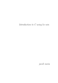
e high level structure of our functional compiler is described by the following block diagram. Each
describes a phase which is a sequence of transformations composed to transform the input program.
9
•
•
•
•
Source - e frontend textual source language.
Parsing - Source is parsed into an abstract syntax tree.
Desugar - Redundant structure from the frontend language is removed and canonicalized.
Type Checking - e program is type-checked and/or type-inferred yielding an explicitly typed
form.
• Transformation - e core language is transformed to prepare for compilation.
• Compilation - e core language is lowered into a form to be compiled or interpreted.
• (Code Generation) - Platform specific code is generated, linked into a binary.
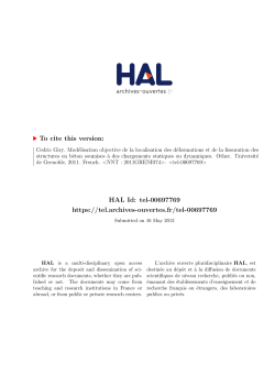
A pass may transform the input program from one form into another or alter the internal state of the
compiler context. e high level description of the forms our final compiler will go through is the
following sequence:
Internal forms used during compilation are intermediate representations and typically any non-trivial language will involve several.
Parsing
e source code is simply the raw sequence of text that specifies the program. Lexing splits the text
stream into a sequence of tokens. Only the presence of invalid symbols is enforced, otherwise meaningless
programs are accepted. Whitespace is either ignored or represented as a unique token in the stream.
let f x = x + 1
For instance the previous program might generate a token stream like the following:
[
TokenLet,
TokenSym ”f”,
TokenSym ”x”,
TokenEq,
TokenSym ”x”,
10
TokenAdd,
TokenNum 1
]
We can then scan the token stream via and dispatch on predefined patterns of tokens called productions
and recursively build up a datatype for the abstract syntax tree (AST) by traversal of the input stream and
generation of the appropriate syntactic.
type Name = String
data Expr
= Var Name
| Lit Lit
| Op PrimOp [Expr]
| Let Name [Name] Expr
data Lit
= LitInt Int
data PrimOp
= Add
So for example the following string is parsed into the resulting Expr value.
let f x = x + 1
Let ”f” [”x”] (Op Add [Var ”x”, Lit (LitInt 1)])
Desugaring
Desugaring is the process by which the frontend AST is transformed into a simpler form of itself by
reducing the number of complex structures by expressing them in terms of a fixed set of simpler constructs.
Haskell’s frontend is very large and many constructs are simplified down. For example where clauses
and operation sections are the most common examples. Where clauses are effectively syntactic sugar for
let bindings and operator sections are desugared into lambdas with the left or right hand side argument
assigned to a fresh variable.
Type Inference
Type inference is the process by which the untyped syntax is endowed with type information by a process
known as type reconstruction or type inference. e inference process may take into account explicit user
annotated types.
11
let f x = x + 1
Let ”f” [] (Lam ”x” (Op Add [Var ”x”, Lit (LitInt 1)]))
Inference will generate a system of constraints which are solved via a process known as unification to yield
the type of the expression.
Int -> Int -> Int
b ~ Int -> c
~
a -> b
f :: Int -> Int
In some cases this type will be incorporated directly into the AST and the inference will transform the
frontend language into an explicitly typed core language.
Let ”f” []
(Lam ”x”
(TArr TInt TInt)
(App
(App
(Prim ”primAdd”) (Var ”x”))
(Lit (LitInt 1))))
Transformation
e type core representation is often suitable for evaluation, but quite often different intermediate representations are more amenable to certain optimizations and make explicit semantic properties of the
language explicit. ese kind of intermediate forms will often attach information about free variables,
allocations, and usage information directly onto the AST to make it
e most important form we will use is called the Spineless Tagless G-Machine ( STG ), an abstract machine
that makes many of the properties of lazy evaluation explicit directly in the AST.
Code Generation
From the core language we will either evaluate it on top of a high-level interpreter written in Haskell
itself, or into another intermediate language like C or LLVM which can itself be compiled into native
code.
let f x = x + 1
Quite often this process will involve another intermediate representation which abstracts over the process
of assigning and moving values between CPU registers and main memory. LLVM and GHC’s Cmm are
two target languages serving this purpose.
12
f:
mov res, arg
add res, 1
ret
define i32 @f(i32 %x) {
entry:
%add = add nsw i32 %x, 1
ret i32 %add
}
From here the target language can be compiled into the system’s assembly language. All code that is
required for evaluation is linked into the resulting module.
f:
movl
movl
addl
movl
ret
%edi, -4(%rsp)
-4(%rsp), %edi
$1, %edi
%edi, %eax
And ultimately this code will be assembled into platform specific instructions by the native code generator,
encoded as a predefined sequence of CPU instructions defined by the processor specification.
0000000000000000
0:
89 7c 24
4:
8b 7c 24
8:
81 c7 01
e:
89 f8
10:
c3
<f>:
fc
fc
00 00 00
mov
mov
add
mov
retq
%edi,-0x4(%rsp)
-0x4(%rsp),%edi
$0x1,%edi
%edi,%eax
13
Haskell Basics
Let us now survey a few of the core concepts that will be used throughout the text. is will be a very
fast and informal discussion. If you are familiar with all of these concepts then it is very likely you will
be able to read the entirety of this tutorial and focus on the subject domain and not the supporting
code. e domain material itself should largely be accessible to an ambitious high school student or
undergraduate; and requires nothing more than a general knowledge of functional programming.
Functions
Functions are the primary building block of all of Haskell logic.
add :: Integer -> Integer -> Integer
add x y = x + y
In Haskell all functions are pure, the only thing a function may do is return a value.
In Haskell all functions are pure. e only thing a function may do is return a value.
All functions in Haskell are curried. For example, when a function of three arguments receives less than
three arguments, it yields a partially applied function, which, when given additional arguments, yields
yet another function or the resulting value if all the arguments were supplied.
g :: Int -> Int -> Int -> Int
g x y z = x + y + z
h :: Int -> Int
h = g 2 3
Haskell supports higher-order functions, i.e., functions which take functions and yield other functions.
compose f g = \x -> f (g x)
iterate :: (a -> a) -> a -> [a]
iterate f x = x : (iterate f (f x))
14
Datatypes
Constructors for datatypes come in two flavors: sum types and product types.
A sum type consists of multiple options of type constructors under the same type. e two cases can be
used at all locations the type is specified, and are discriminated using pattern matching.
data Sum = A Int | B Bool
A product type combines multiple typed fields into the same type.
data Prod = Prod Int Bool
Records are a special product type that, in addition to generating code for the constructors, generates a
special set of functions known as selectors which extract the values of a specific field from the record.
data Prod = Prod { a :: Int , b :: Bool }
-- a :: Prod -> Int
-- b :: Prod -> Bool
Sums and products can be combined.
data T1
= A Int Int
| B Bool Bool
e fields of a datatype may be parameterized, in which case the type depends on the specific types the
fields are instantiated with.
data Maybe a = Nothing | Just a
Values
A list is a homogeneous, inductively defined sum type of linked cells parameterized over the type of its
values.
data List a = Nil | Cons a (List a)
a = [1,2,3]
a = Cons 1 (Cons 2 (Cons 3 Nil))
List have special value-level syntax:
15
(:) = Cons
[] = Nil
(1 : (2 : (3 : []))) = [1,2,3]
A tuple is a heterogeneous product type parameterized over the types of its two values.
Tuples also have special value-level syntax.
data Pair a b = Pair a b
a = (1,2)
a = Pair 1 2
(,) = Pair
Tuples are allowed (with compiler support) to have up to 15 fields in GHC.
Pattern matching
Pattern matching allows us to discriminate on the constructors of a datatype, mapping separate cases to
separate code paths.
data Maybe a = Nothing | Just a
maybe :: b -> (a -> b) -> Maybe a -> b
maybe n f Nothing = n
maybe n f (Just a) = f a
Top-level pattern matches can always be written identically as case statements.
maybe :: b -> (a -> b) -> Maybe a -> b
maybe n f x = case x of
Nothing -> n
Just a -> f a
Wildcards can be placed for patterns where the resulting value is not used.
const :: a -> b -> a
const x _ = x
List and tuples have special pattern syntax.
16
length :: [a] -> Int
length []
= 0
length (x:xs) = 1 + (length xs)
fst :: (a, b) -> a
fst (a,b) = a
Patterns may be guarded by predicates (functions which yield a boolean). Guards only allow the execution of a branch if the corresponding predicate yields True.
filter :: (a -> Bool) -> [a] -> [a]
filter pred []
= []
filter pred (x:xs)
| pred x
= x : filter pred xs
| otherwise
=
filter pred xs
Recursion
In Haskell all iteration over data structures is performed by recursion. Entering a function in Haskell
does not create a new stack frame, the logic of the function is simply entered with the arguments on the
stack and yields result to the register. In the case where a function returns a invocation of itself invoked
in the tail position the resulting logic is compiled identically to while loops in other languages, via a jmp
instruction instead of a call.
sum :: [Int] -> [Int]
sum ys = go ys 0
where
go (x:xs) i = go xs (i+x)
go [] i = i
Functions can be defined to recurse mutually on each other.
even 0 = True
even n = odd (n-1)
odd 0 = False
odd n = even (n-1)
Laziness
A Haskell program can be thought of as being equivalent to a large directed graph. Each edge represents
the use of a value, and each node is the source of a value. A node can be:
17
• A thunk, i.e., the application of a function to values that have not been evaluated yet
• A thunk that is currently being evaluated, which may induce the evaluation of other thunks in the
process
• An expression in weak head normal form, which is only evaluated to the outermost constructor or
lambda abstraction
e runtime has the task of determining which thunks are to be evaluated by the order in which they
are connected to the main function node. is is the essence of all evaluation in Haskell and is called
graph reduction.
Self-referential functions are allowed in Haskell. For example, the following functions generate infinite
lists of values. However, they are only evaluated up to the depth that is necessary.
-- Infinite stream of 1’s
ones = 1 : ones
-- Infinite count from n
numsFrom n = n : numsFrom (n+1)
-- Infinite stream of integer squares
squares = map (^2) (numsfrom 0)
e function take consumes an infinite stream and only evaluates the values that are needed for the
computation.
take
take
take
take
:: Int -> [a]
n _ | n <= 0
n []
n (x:xs)
->
=
=
=
[a]
[]
[]
x : take (n-1) xs
take 5 squares
-- [0,1,4,9,16]
is also admits diverging terms (called bottoms), which have no normal form. Under lazy evaluation,
these values can be threaded around and will never diverge unless actually forced.
bot = bot
So, for instance, the following expression does not diverge since the second argument is not used in the
body of const.
const 42 bot
e two bottom terms we will use frequently are used to write the scaffolding for incomplete programs.
error :: String -> a
undefined :: a
18
Higher-Kinded Types
e “type of types” in Haskell is the language of kinds. Kinds are either an arrow (* -> *) or a star (*).
e kind of an Int is *, while the kind of Maybe is * -> *. Haskell supports higher-kinded types, which
are types that take other types and construct a new type. A type constructor in Haskell always has a kind
which terminates in a *.
-- T1 :: (* -> *) -> * -> *
data T1 f a = T1 (f a)
e three special types (,), (->), [] have special type-level syntactic sugar:
(,) Int Int
(->) Int Int
[] Int
=
=
=
(Int, Int)
Int -> Int
[Int]
Typeclasses
A typeclass is a collection of functions which conform to a given interface. An implementation of an
interface is called an instance. Typeclasses are effectively syntactic sugar for records of functions and
nested records (called dictionaries) of functions parameterized over the instance type. ese dictionaries
are implicitly threaded throughout the program whenever an overloaded identifier is used. When a
typeclass is used over a concrete type, the implementation is simply spliced in at the call site. When a
typeclass is used over a polymorphic type, an implicit dictionary parameter is added to the function so
that the implementation of the necessary functionality is passed with the polymorphic value.
Typeclasses are “open” and additional instances can always be added, but the defining feature of a typeclass is that the instance search always converges to a single type to make the process of resolving overloaded identifiers globally unambiguous.
For instance, the Functor typeclass allows us to “map” a function generically over any type of kind (* ->
*) and apply it to its internal structure.
class Functor f where
fmap :: (a -> b) -> f a -> f b
instance Functor [] where
fmap f []
= []
fmap f (x:xs) = f x : fmap f xs
instance Functor ((,) a) where
fmap f (a,b) = (a, f b)
19
Operators
In Haskell, infix operators are simply functions, and quite often they are used in place of alphanumerical
names when the functions involved combine in common ways and are subject to algebraic laws.
infixl
infixl
infixl
infixl
6
6
7
7
+
/
*
infixr 5 ++
infixr 9 .
Operators can be written in section form:
(x+) =
(+y) =
(+) =
\y -> x+y
\x -> x+y
\x y -> x+y
Any binary function can be written in infix form by surrounding the name in backticks.
(+1) ‘fmap‘ [1,2,3] -- [2,3,4]
Monads
A monad is a typeclass with two functions: bind and return.
class Monad m where
bind
:: m a -> (a -> m b) -> m b
return :: a -> m a
e bind function is usually written as an infix operator.
infixl 1 >>=
class Monad m where
(>>=) :: m a -> (a -> m b) -> m b
return :: a -> m a
is defines the structure, but the monad itself also requires three laws that all monad instances must
satisfy.
Law 1
20
return a >>= f = f a
Law 2
m >>= return = m
Law 3
(m >>= f) >>= g = m >>= (\x -> f x >>= g)
Haskell has a level of syntactic sugar for monads known as do-notation. In this form, binds are written
sequentially in block form which extract the variable from the binder.
do { a <- f ; m } = f >>= \a -> do { m }
do { f ; m } = f >> do { m }
do { m } = m
So, for example, the following are equivalent:
do
a <- f
b <- g
c <- h
return (a, b, c)
f >>= \a ->
g >>= \b ->
h >>= \c ->
return (a, b, c)
Applicatives
Applicatives allow sequencing parts of some contextual computation, but do not bind variables therein.
Strictly speaking, applicatives are less expressive than monads.
class Functor f => Applicative f where
pure :: a -> f a
(<*>) :: f (a -> b) -> f a -> f b
(<$>) :: Functor f => (a -> b) -> f a -> f b
(<$>) = fmap
Applicatives satisfy the following laws:
21
pure id <*> v = v
pure f <*> pure x = pure (f x)
u <*> pure y = pure ($ y) <*> u
u <*> (v <*> w) = pure (.) <*> u <*> v <*> w
-----
Identity
Homomorphism
Interchange
Composition
For example:
example1
example1
where
m1 =
m2 =
:: Maybe Integer
= (+) <$> m1 <*> m2
Just 3
Nothing
Instances of the Applicative typeclass also have available the functions *> and <*. ese functions
sequence applicative actions while discarding the value of one of the arguments. e operator *> discards
the left argument, while <* discards the right. For example, in a monadic parser combinator library, the
*> would discard the value of the first argument but return the value of the second.
Monoids
class Monoid a where
mempty :: a
mappend :: a -> a -> a
mconcat :: [a] -> a
Deriving
Instances for typeclasses like Read, Show, Eq and Ord can be derived automatically by the Haskell compiler.
data PlatonicSolid
= Tetrahedron
| Cube
| Octahedron
| Dodecahedron
| Icosahedron
deriving (Show, Eq, Ord, Read)
example
example
example
example
=
=
=
=
show
read
Cube
sort
Icosahedron
”Tetrahedron”
== Octahedron
[Cube, Dodecahedron]
22
IO
A value of type IO a is a computation which, when performed, does some I/O before returning a value
of type a. e notable feature of Haskell is that IO is still functionally pure; a value of type IO a is
simply a value which stands for a computation which, when invoked, will perform IO. ere is no way
to peek into its contents without running it.
For instance, the following function does not print the numbers 1 to 5 to the screen. Instead, it builds
a list of IO computations:
fmap print [1..5] :: [IO ()]
We can then manipulate them as an ordinary list of values:
reverse (fmap print [1..5]) :: [IO ()]
We can then build a composite computation of each of the IO actions in the list using sequence_,
which will evaluate the actions from left to right. e resulting IO computation can be evaluated in
main (or the GHCi repl, which effectively is embedded inside of IO).
>> sequence_ (fmap print [1..5]) :: IO ()
1
2
3
4
5
>> sequence_ (reverse (fmap print [1..5])) :: IO ()
5
4
3
2
1
e IO monad is a special monad wired into the runtime. It is a degenerate case and most monads in
Haskell have nothing to do with effects in this sense.
putStrLn :: String -> IO ()
print
:: Show a => a -> IO ()
e type of main is always IO ().
main :: IO ()
main = do
putStrLn ”Enter a number greater than 3: ”
x <- readLn
print (x > 3)
23
e essence of monadic IO in Haskell is that effects are reified as first class values in the language and reflected
in the type system. is is one of foundational ideas of Haskell, although it is not unique to Haskell.
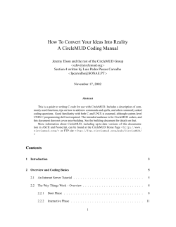
Monad Transformers
Monads can be combined together to form composite monads. Each of the composite monads consists
of layers of different monad functionality. For example, we can combine an error-reporting monad with
a state monad to encapsulate a certain set of computations that need both functionalities. e use of
monad transformers, while not always necessary, is often one of the primary ways to structure modern
Haskell programs.
class MonadTrans t where
lift :: Monad m => m a -> t m a
e implementation of monad transformers is comprised of two different complementary libraries,
transformers and mtl. e transformers library provides the monad transformer layers and mtl
extends this functionality to allow implicit lifting between several layers.
To use transformers, we simply import the Trans variants of each of the layers we want to compose and
then wrap them in a newtype.
{-# LANGUAGE GeneralizedNewtypeDeriving #-}
import Control.Monad.Trans
import Control.Monad.Trans.State
import Control.Monad.Trans.Writer
newtype Stack a = Stack { unStack :: StateT Int (WriterT [Int] IO) a }
deriving (Monad)
foo :: Stack ()
foo = Stack $ do
put 1
lift $ tell [2]
lift $ lift $ print 3
return ()
-- State layer
-- Writer layer
-- IO Layer
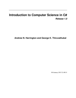
evalStack :: Stack a -> IO [Int]
evalStack m = execWriterT (evalStateT (unStack m) 0)
As illustrated by the following stack diagram:
Using mtl and GeneralizedNewtypeDeriving, we can produce the same stack but with a simpler
forward-facing interface to the transformer stack. Under the hood, mtl is using an extension called
FunctionalDependencies to automatically infer which layer of a transformer stack a function belongs
to and can then lift into it.
24
{-# LANGUAGE GeneralizedNewtypeDeriving #-}
import Control.Monad.Trans
import Control.Monad.State
import Control.Monad.Writer
newtype Stack a = Stack { unStack :: StateT Int (WriterT [Int] IO) a }
deriving (Monad, MonadState Int, MonadWriter [Int], MonadIO)
foo :: Stack ()
foo = do
put 1
tell [2]
liftIO $ print 3
return ()
-- State layer
-- Writer layer
-- IO Layer
evalStack :: Stack a -> IO [Int]
evalStack m = execWriterT (evalStateT (unStack m) 0)
StateT
e state monad allows functions within a stateful monadic context to access and modify shared state.
put
get
gets
modify
::
::
::
::
s -> State s ()
State s s
(s -> a) -> State s a
(s -> s) -> State s ()
-----
set the
get the
apply a
set the
state value
state
function over the state, and return the result
state, using a modifier function
Evaluation functions often follow the naming convention of using the prefixes run, eval, and exec:
execState :: State s a -> s -> s
evalState :: State s a -> s -> a
runState :: State s a -> s -> (a, s)
-- yield the state
-- yield the return value
-- yield the state and return value
25
For example:
import Control.Monad.State
test :: State Int Int
test = do
put 3
modify (+1)
get
main :: IO ()
main = print $ execState test 0
ReaderT
e Reader monad allows a fixed value to be passed around inside the monadic context.
ask
:: Reader r r
local :: (r -> r) -> Reader r a -> Reader r a
-- get the value
-- run a monadic action, with the value modified by
For example:
import Control.Monad.Reader
data MyContext = MyContext
{ foo :: String
, bar :: Int
} deriving (Show)
computation :: Reader MyContext (Maybe String)
computation = do
n <- asks bar
x <- asks foo
if n > 0
then return (Just x)
else return Nothing
ex1 :: Maybe String
ex1 = runReader computation $ MyContext ”hello” 1
ex2 :: Maybe String
ex2 = runReader computation $ MyContext ”haskell” 0
WriterT
e writer monad lets us emit a lazy stream of values from within a monadic context. e primary
function tell adds a value to the writer context.
26
tell :: (Monoid w) => w -> Writer w ()
e monad can be devalued with or without the collected values.
execWriter :: (Monoid w) => Writer w a -> w
runWriter :: (Monoid w) => Writer w a -> (a, w)
import Control.Monad.Writer
type MyWriter = Writer [Int] String
example :: MyWriter
example = do
tell [1..5]
tell [5..10]
return ”foo”
output :: (String, [Int])
output = runWriter example
ExceptT
e Exception monad allows logic to fail at any point during computation with a user-defined exception.
e exception type is the first parameter of the monad type.
throwError :: e -> Except e a
runExcept :: Except e a -> Either e a
For example:
import Control.Monad.Except
type Err = String
safeDiv :: Int -> Int -> Except Err Int
safeDiv a 0 = throwError ”Divide by zero”
safeDiv a b = return (a ‘div‘ b)
example :: Either Err Int
example = runExcept $ do
x <- safeDiv 2 3
y <- safeDiv 2 0
return (x + y)
27
Kleisli Arrows
An additional combinator for monads composes two different monadic actions in sequence. It is the
monadic equivalent of the regular function composition operator (.).
(>=>) :: Monad m => (a -> m b) -> (b -> m c) -> a -> m c
e monad laws can be expressed equivalently in terms of Kleisli composition.
(f >=> g) >=> h
return >=> f
f >=> return
=
=
=
f >=> (g >=> h)
f
f
Text
e usual String type is a singly-linked list of characters, which, although simple, is not efficient in
storage or locality. e letters of the string are not stored contiguously in memory and are instead
allocated across the heap.
e Text and ByteString libraries provide alternative efficient structures for working with contiguous
blocks of text data. ByteString is useful when working with the ASCII character set, while Text
provides a text type for use with Unicode.
e OverloadedStrings extension allows us to overload the string type in the frontend language to
use any one of the available string representations.
class IsString a where
fromString :: String -> a
pack :: String -> Text
unpack :: Text -> String
So, for example:
{-# LANGUAGE OverloadedStrings #-}
import qualified Data.Text as T
str :: T.Text
str = ”bar”
Cabal
To set up an existing project with a sandbox, run:
$ cabal sandbox init
28
is will create the .cabal-sandbox directory, which is the local path GHC will use to look for dependencies when building the project.
To install dependencies from Hackage, run:
$ cabal install --only-dependencies
Finally, configure the library for building:
$ cabal configure
Now we can launch a GHCi shell scoped with the modules from the project in scope:
$ cabal repl
Resources
If any of these concepts are unfamiliar, there are some external resources that will try to explain them.
e most thorough is probably the Stanford course lecture notes.
• Stanford CS240h by Bryan O’Sullivan, David Terei
• Real World Haskell by Bryan O’Sullivan, Don Stewart, and John Goerzen
ere are some books as well, but your mileage may vary with these. Much of the material is dated and
only covers basic functional programming and not “programming in the large”.
• Learn you a Haskell by Miran Lipovača
• Programming in Haskell by Graham Hutton
• inking Functionally by Richard Bird
29
Parsing
Parser Combinators
For parsing in Haskell it is quite common to use a family of libraries known as parser combinators which
let us compose higher order functions to generate parsers. Parser combinators are a particularly expressive
pattern that allows us to quickly prototype language grammars in an small embedded domain language
inside of Haskell itself. Most notably we can embed custom Haskell logic inside of the parser.
NanoParsec
So now let’s build our own toy parser combinator library which we’ll call NanoParsec just to get the feel
of how these things are built.
{-# OPTIONS_GHC -fno-warn-unused-do-bind #-}
module NanoParsec where
import Data.Char
import Control.Monad
import Control.Applicative
Structurally a parser is a function which takes an input stream of characters and yields an parse tree by
applying the parser logic over sections of the character stream (called lexemes) to build up a composite
data structure for the AST.
newtype Parser a = Parser { parse :: String -> [(a,String)] }
Running the function will result in traversing the stream of characters yielding a resultant AST structure
for the type variable a, or failing with a parse error for malformed input, or failing by not consuming the
entire stream of input. A more robust implementation would track the position information of failures
for error reporting.
runParser :: Parser a -> String -> a
runParser m s =
30
case parse m s of
[(res, [])] -> res
[(_, rs)]
-> error ”Parser did not consume entire stream.”
[]
-> error ”Parser error.”
Recall that in Haskell in the String type is itself defined to be a list of Char values, so the following are
equivalent forms of the same data.
”1+2*3”
[’1’, ’+’, ’2’, ’*’, ’3’]
We advance the parser by extracting a single character from the parser stream and returning in a tuple
containing itself and the rest of the stream. e parser logic will then scrutinize the character and either
transform it in some portion of the output or advance the stream and proceed.
item :: Parser Char
item = Parser $ \s ->
case s of
[]
-> []
(c:cs) -> [(c,cs)]
A bind operation for our parser type will take one parse operation and compose it over the result of
second parse function. Since the parser operation yields a list of tuples, composing a second parser
function simply maps itself over the resulting list and concat’s the resulting nested list of lists into a
single flat list in the usual list monad fashion. e unit operation injects a single pure value into the
parse stream.
bind :: Parser a -> (a -> Parser b) -> Parser b
bind p f = Parser $ \s -> concatMap (\(a, s’) -> parse (f a) s’) $ parse p s
unit :: a -> Parser a
unit a = Parser (\s -> [(a,s)])
As the terminology might have indicated this is indeed a Monad (also Functor and Applicative).
instance Functor Parser where
fmap f (Parser cs) = Parser (\s -> [(f a, b) | (a, b) <- cs s])
instance Applicative Parser where
pure = return
(Parser cs1) <*> (Parser cs2) = Parser (\s -> [(f a, s2) | (f, s1) <- cs1 s, (a, s2) <- cs2 s1])
31
instance Monad Parser where
return = unit
(>>=) = bind
Of particular importance is that this particular monad has a zero value (failure), namely the function
which halts reading the stream and returns the empty stream. Together this forms a monoidal structure
with a secondary operation (combine) which applies two parser functions over the same stream and
concatenates the result. Together these give rise to both the Alternative and MonadPlus class instances
which encode the logic for trying multiple parse functions over the same stream and handling failure
and rollover.
e core operator introduced here is (<|>) operator for combining two optional paths of parser logic,
switching to second path if the first fails with the zero value.
instance MonadPlus Parser where
mzero = failure
mplus = combine
instance Alternative Parser where
empty = mzero
(<|>) = option
combine :: Parser a -> Parser a -> Parser a
combine p q = Parser (\s -> parse p s ++ parse q s)
failure :: Parser a
failure = Parser (\cs -> [])
option :: Parser a -> Parser a -> Parser a
option p q = Parser $ \s ->
case parse (mplus p q) s of
[]
-> []
(x:xs) -> [x]
Derived automatically from the Alternative typeclass definition is the many and some functions. Many
takes a single function argument and repeatedly applies it until the function fails and then yields the
collected results up to that point. e some function behaves similar except that it will fail itself if there
is not at least a single match.
-- | One or more.
some :: f a -> f [a]
some v = some_v
where
32
many_v = some_v <|> pure []
some_v = (:) <$> v <*> many_v
-- | Zero or more.
many :: f a -> f [a]
many v = many_v
where
many_v = some_v <|> pure []
some_v = (:) <$> v <*> many_v
On top of this we can add functionality for checking whether the current character in the stream matches
a given predicate ( i.e is it a digit, is it a letter, a specific word, etc).
satisfy :: (Char -> Bool) -> Parser Char
satisfy p = item ‘bind‘ \c ->
if p c
then unit c
else (Parser (\cs -> []))
Essentially this 50 lines code encodes the entire core of the parser combinator machinery. All higher
order behavior can be written on top of just this logic. Now we can write down several higher level
functions which operate over sections of the stream.
chainl1 parses one or more occurrences of p, separated by op and returns a value obtained by a recursing
until failure on the left hand side of the stream. is can be used to parse left-recursive grammar.
oneOf :: [Char] -> Parser Char
oneOf s = satisfy (flip elem s)
chainl :: Parser a -> Parser (a -> a -> a) -> a -> Parser a
chainl p op a = (p ‘chainl1‘ op) <|> return a
chainl1 :: Parser a -> Parser (a -> a -> a) -> Parser a
p ‘chainl1‘ op = do {a <- p; rest a}
where rest a = (do f <- op
b <- p
rest (f a b))
<|> return a
Using satisfy we can write down several combinators for detecting the presence of specific common
patterns of characters ( numbers, parenthesized expressions, whitespace, etc ).
char :: Char -> Parser Char
char c = satisfy (c ==)
33
natural :: Parser Integer
natural = read <$> some (satisfy isDigit)
string :: String -> Parser String
string [] = return []
string (c:cs) = do { char c; string cs; return (c:cs)}
token :: Parser a -> Parser a
token p = do { a <- p; spaces ; return a}
reserved :: String -> Parser String
reserved s = token (string s)
spaces :: Parser String
spaces = many $ oneOf ” \n\r”
digit :: Parser Char
digit = satisfy isDigit
number :: Parser Int
number = do
s <- string ”-” <|> return []
cs <- some digit
return $ read (s ++ cs)
parens :: Parser a -> Parser a
parens m = do
reserved ”(”
n <- m
reserved ”)”
return n
And that’s about it! In a few hundred lines we have enough of a parser library to write down a simple
parser for a calculator grammar. In the formal Backus–Naur Form our grammar would be written as:
number
digit
expr
term
factor
addop
mulop
=
=
=
=
=
=
=
[ ”-” ] digit { digit }.
”0” | ”1” | ... | ”8” | ”9”.
term { addop term }.
factor { mulop factor }.
”(” expr ”)” | number.
”+” | ”-”.
”*”.
e direct translation to Haskell in terms of our newly constructed parser combinator has the following
form:
34
data Expr
= Add Expr Expr
| Mul Expr Expr
| Sub Expr Expr
| Lit Int
deriving Show
eval ::
eval ex
Add a
Mul a
Sub a
Lit n
Expr -> Int
= case ex of
b -> eval a + eval b
b -> eval a * eval b
b -> eval a - eval b
-> n
int :: Parser Expr
int = do
n <- number
return (Lit n)
expr :: Parser Expr
expr = term ‘chainl1‘ addop
term :: Parser Expr
term = factor ‘chainl1‘ mulop
factor :: Parser Expr
factor =
int
<|> parens expr
infixOp :: String -> (a -> a -> a) -> Parser (a -> a -> a)
infixOp x f = reserved x >> return f
addop :: Parser (Expr -> Expr -> Expr)
addop = (infixOp ”+” Add) <|> (infixOp ”-” Sub)
mulop :: Parser (Expr -> Expr -> Expr)
mulop = infixOp ”*” Mul
run :: String -> Expr
run = runParser expr
main :: IO ()
main = forever $ do
putStr ”> ”
a <- getLine
35
print $ eval $ run a
Now we can try out our little parser.
$ runhaskell parsec.hs
> 1+2
3
> 1+2*3
7
Generalizing String
e limitations of the String type are well-known, but what is particularly nice about this approach is
that it is adapts to different stream type simply by adding an additional parameter to the Parser type
which holds the stream type. In place a more efficient data structure like Data.Text can replaced.
newtype Parser s a = Parser { parse :: s -> [(a,s)] }
For the first couple of simple parsers we will use the String type for simplicity’s sake, but later will
generalize our parsers to use the Text type. e combinators and parsing logic will not change, only the
lexer and language definitions types will change slightly to a generalized form.
Parsec
Now that we have the feel for parser combinators work, we can graduate to full the Parsec library. We’ll
effectively ignore the gritty details of parsing and lexing from here out. Although an interesting subject
parsing is effectively a solved problem and the details are not terribly important for our purposes.
e Parsec library defines a set of common combinators much like the operators we defined in our toy
library.
Combinator
Description
char
string
<|>
Match the given character.
Match the given string.
e choice operator tries to parse the first argument before
proceeding to the second. Can be chained sequentially to a
generate a sequence of options.
Consumes an arbitrary number of patterns matching the given
pattern and returns them as a list.
Like many but requires at least one match.
Match a arbitrary length sequence of patterns, delimited by
a given pattern.
Optionally parses a given pattern returning its value as a
Maybe.
Backtracking operator will let us parse ambiguous matching
expressions and restart with a different pattern.
36 surrounded by parentheses.
Parsers the given pattern
many
many1
sepBy
optional
try
parens
Tokens
To create a Parsec lexer we must first specify several parameters about how individual characters are
handled and converted into tokens. For example some tokens will be handled as comments and simply
omitted from the parse stream. Other parameters include indicating what characters are to be handled
as keyword identifiers or operators.
langDef :: Tok.LanguageDef ()
langDef = Tok.LanguageDef
{ Tok.commentStart
= ”{-”
, Tok.commentEnd
= ”-}”
, Tok.commentLine
= ”--”
, Tok.nestedComments = True
, Tok.identStart
= letter
, Tok.identLetter
= alphaNum <|> oneOf ”_’”
, Tok.opStart
= oneOf ”:!#$%&*+./<=>?@\\^|-~”
, Tok.opLetter
= oneOf ”:!#$%&*+./<=>?@\\^|-~”
, Tok.reservedNames
= reservedNames
, Tok.reservedOpNames = reservedOps
, Tok.caseSensitive
= True
}
Lexer
Given the token definition we can create the lexer functions.
lexer :: Tok.TokenParser ()
lexer = Tok.makeTokenParser langDef
parens :: Parser a -> Parser a
parens = Tok.parens lexer
reserved :: String -> Parser ()
reserved = Tok.reserved lexer
semiSep :: Parser a -> Parser [a]
semiSep = Tok.semiSep lexer
reservedOp :: String -> Parser ()
reservedOp = Tok.reservedOp lexer
infixOp :: String -> (a -> a) -> Ex.Operator String () Identity a
infixOp s f = Ex.Prefix (reservedOp s >> return f)
Abstract Syntax Tree
In a separate module we’ll now define the abstract syntax for our language as a datatype.
37
module Syntax where
data Expr
= Tr
| Fl
| Zero
| IsZero Expr
| Succ Expr
| Pred Expr
| If Expr Expr Expr
deriving (Eq, Show)
Parser
Much like before our parser is simply written in monadic blocks, each mapping a a set of patterns to a
construct in our Expr type. e toplevel entry point to our parser is the expr function which we can
parse with by using the Parsec function parse.
infixOp s f = Ex.Prefix (reservedOp s >> return f)
-- Infix operators
table :: Ex.OperatorTable String () Identity Expr
table = [
[
infixOp ”succ” Succ
, infixOp ”pred” Pred
, infixOp ”iszero” IsZero
]
]
-- if/then/else
ifthen :: Parser Expr
ifthen = do
reserved ”if”
cond <- expr
reservedOp ”then”
tr <- expr
reserved ”else”
fl <- expr
return (If cond tr fl)
-- Constants
true, false, zero :: Parser Expr
true = reserved ”true” >> return Tr
38
false = reserved ”false” >> return Fl
zero = reservedOp ”0”
>> return Zero
expr :: Parser Expr
expr = Ex.buildExpressionParser table factor
factor :: Parser Expr
factor =
true
<|> false
<|> zero
<|> ifthen
<|> parens expr
contents :: Parser a -> Parser a
contents p = do
Tok.whiteSpace lexer
r <- p
eof
return r
e toplevel function we’ll expose from our Parse module is the parseExpr which will be called as the
entry point in our REPL.
parseExpr s = parse (contents expr) ”<stdin>” s
Evaluation
Our small language gives rise has two syntactic classes, values and expressions. Values are in normal form
and cannot be reduced further. ese consist of True and False values and literal numbers.
isNum Zero
= True
isNum (Succ t) = isNum t
isNum _
= False
isVal
isVal
isVal
isVal
isVal
:: Expr -> Bool
Tr = True
Fl = True
t | isNum t = True
_ = False
e evaluation of our languages uses the Maybe applicative to accommodate the fact that our reduction
may halt at any level with a Nothing if the expression being reduced has reached a normal form or
39
cannot proceed because the reduction simply isn’t well-defined. e rules for evaluation are a single step
by which an expression takes a single small step one from form to another by a given rule.
eval’ x = case x of
IsZero Zero
-> Just Tr
IsZero (Succ t) | isNum t -> Just Fl
IsZero t
-> IsZero <$> (eval’ t)
Succ t
-> Succ <$> (eval’ t)
Pred Zero
-> Just Zero
Pred (Succ t) | isNum t
-> Just t
Pred t
-> Pred <$> (eval’ t)
If Tr c _
-> Just c
If Fl _ a
-> Just a
If t c a
-> (\t’ -> If t’ c a) <$> eval’ t
_
-> Nothing
At the toplevel we simply apply the nf repeatedly until either a value is reached or we’re left with an
expression that has no well-defined way to proceed. e term is “stuck” and the program is an undefined
state.
nf x = fromMaybe x (nf <$> eval’ x)
eval :: Expr -> Maybe Expr
eval t = case isVal (nf t) of
True -> Just (nf t)
False -> Nothing -- term is ”stuck”
REPL
e driver for our simple language simply invokes all of the parser and evaluation logic in a loop feeding
the resulting state to the next iteration. We will use the haskeline library to give us readline interactions
for the small REPL. Behind the scenes haskeline is using readline or another platform-specific system
library to manage the terminal input. To start out we just create the simplest loop, which only parses
and evaluates expressions and prints them to the screen. We’ll build on this pattern in each chapter,
eventually ending up with a more full-featured REPL.
e two functions of note are the operations for the InputT monad transformer.
runInputT :: Settings IO -> InputT IO a -> IO a
getInputLine :: String -> InputT IO (Maybe String)
When the user enters a EOF or sends a SIGQUIT to input, getInputLine will yield Nothing and can
handle the exit logic.
40
process :: String -> IO ()
process line = do
let res = parseExpr line
case res of
Left err -> print err
Right ex -> print $ runEval ex
main :: IO ()
main = runInputT defaultSettings loop
where
loop = do
minput <- getInputLine ”Repl> ”
case minput of
Nothing -> outputStrLn ”Goodbye.”
Just input -> (liftIO $ process input) >> loop
Soundness
Great, now let’s test our little interpreter and indeed we see that it behaves as expected.
Arith> succ 0
succ 0
Arith> succ (succ 0)
succ (succ 0)
Arith> iszero 0
true
Arith> if false then true else false
false
Arith> iszero (pred (succ (succ 0)))
false
Arith> pred (succ 0)
0
Arith> iszero false
Cannot evaluate
Arith> if 0 then true else false
Cannot evaluate
Oh no, our calculator language allows us to evaluate terms which are syntactically valid but semantically
meaningless. We’d like to restrict the existence of such terms since when we start compiling our languages
41
later into native CPU instructions these kind errors will correspond to all sorts of nastiness (segfaults,
out of bounds errors, etc). How can we make these illegal states unrepresentable to begin with?
Full Source
• NanoParsec
• Calculator
42
at language is an instrument of human reason, and not merely a medium for the expression of
thought, is a truth generally admitted.
— George Boole
Lambda Calculus
Fundamental to all functional languages is the most atomic notion of composition, function abstraction
of a single variable. e lambda calculus consists very simply of three terms and all valid recursive
combinations thereof:
e terms are named are typically referred to in code by the following contractions.
• Var - A variable
• Lam - A lambda abstraction
• App - An application
e := x
(Var)
λx.e (Lam)
ee
(App)
e lambda calculus is often called the “assembly language” of functional programming, and variations
and extensions on it form the basis of many functional compiler intermediate forms for languages like
Haskell, OCaml, StandardML, etc. e variation we will discuss first is known as untyped lambda
calculus, by contrast later we will discuss the typed lambda calculus which is an extension thereof.
A lambda expression is said to bind its enclosing variable. So the lambda here binds the name x.
43
λx.e
ere are several lexical conventions that we will adopt when writing lambda expressions. Application
of multiple lambda expressions associates to the left.
x1 x2 x3 ...xn = (...((x1 x2 )x3 )...xn )
By convention application extends as far to the right as is syntactically meaningful. Parenthesis are used
to disambiguate.
In the lambda calculus all lambdas are of a single argument which may itself return another lambda.
Out of convenience we often express multiple lambda expressions with their variables on one lambda
symbol. is is merely a lexical convention and does not change the underlying meaning.
λxy.z = λx.λy.z
e actual implementation of the lambda calculus admits several degrees of freedom in how they are
represented. e most notable is the choice of identifier for the binding variables. A variable is said to
be bound if it is contained in a lambda expression of the same variable binding. Conversely a variable is
free if it is not bound.
A term with free variables is said to a open term while one without open variables is said to be closed or a
combinator.
e0 = λx.x
e1 = λx.(x(λy.ya)x)y
e0 is a combinator while e1 is not. In e1 both occurances of x are bound. e first y is bound, while the
second is free. a is also free.
Variables that appear multiple times in an expression are only bound by the inner most binder. For
example the x variable in the following expression is bound on the inner lambda, while y is bound on
the outer lambda. is kind of occurrence is referred to as name shadowing.
λxy.(λxz.x + y)
SKI Combinators
ere are several important closed expressions called the SKI combinators.
S = λf.(λg.(λx.f x(gx)))
K = λx.λy.x
I = λx.x
In Haskell these are written simply:
44
s f g x = f x (g x)
k x y = x
i x = x
Rather remarkably Moses Schönfinkel showed that all closed lambda expression can be expressed in
terms of the S and K combinators including the I combinator. For example one can easily show that
SKK reduces to I.
SKK
= ((λxyz.xz(yz))(λxy.x)(λxy.x))
= ((λyz.(λxy.x)z(yz))(λxy.x))
= λz.(λxy.x)z((λxy.x)z)
= λz.(λy.z)((λxy.x)z)
= λz.z
=I
is fact is a useful sanity check when testing an implementation of the lambda calculus.
Omega Combinator
An important degenerate case that we’ll test is the omega combinator which applies a single argument
to itself.
ω = λx.xx
When we apply the ω combinator to itself we find that this results in an equal and infinitely long chain
of reductions. A sequence of reductions that has no normal form ( i.e. it reduces indefinitely ) is said to
diverge.
(λx.xx)(λx.xx) →
(λx.xx)(λx.xx) →
(λx.xx)(λx.xx) . . .
We’ll call this expression the Ω combinator. It is the canonical looping term in the lambda calculus.
Quite a few of our type systems which are statically typed will reject this term from being well-formed,
so it is quite useful tool for testing.
Ω = ωω = (λx.xx)(λx.xx)
Implementation
e simplest implementation of the lambda calculus syntax with named binders, is the following definition.
45
type Name = String
data Expr
= Var Name
| App Expr Expr
| Lam Name Expr
ere are several lexical syntax choices for lambda expressions, we will simply choose the Haskell convention which denotes lambda by the backslash (\) to the body with (->), and application by spaces.
Named variables are simply alphanumeric sequences of characters.
• Logical notation: const = λxy.x
• Haskell notation: const = \x y -> x
In addition other terms like literal numbers or booleans can be added, and these make writing expository
examples a little easier. In addition we will add a Lit constructor.
data Expr
= ...
| Lit Lit
data Lit
= LInt Int
| LBool Bool
Substitution
Evaluation of a lambda term ((λx.e)a) proceeds by substitution of all occurrences of the variable x
with the argument a in e. A single substitution step is called a reduction. We write the substitution
application in brackets before the expression it is to be applied over, [x/a]e maps the variable x to the
new replacement a over the expression e.
(λx.e)a → [x/a]e
A substitution metavariable will be written as [s].
e fundamental issue with using locally named binders is the problem of name capture, or how to handle
the case where a substitution conflicts with the names of free variables. For instance naive substitution
would fundamentally alter the meaning of the following expression when y is rewritten to x.
[y/x](λy.yx) → λx.xx
By convention we will always use a capture-avoiding substitution. Substitution will only proceed if the
variable is not in the set of free variables of the expression, and if it does then a fresh variable will be
created in its place.
46
(λx.e)a → [x/a]e
if x ∈
/ fv(e)
ere are several binding libraries and alternative implementations of the lambda calculus syntax that
avoid these problems. It is a very common problem and it is very easy to implement incorrectly even for
experts.
Conversion and Equivalences
Alpha equivelance
α
(λx.e) = (λy.[x/y]e)
Alpha equivalence is the property ( when using named binders ) that changing the variable on the binder
and throughout the body of the expression should not change the fundamental meaning of the whole
expression. So for example the following are alpha-equivalent.
λxy.xy
α
=
λab.ab
Beta-reduction
Beta reduction is simply a single substitution step, replacing a variable bound by a lambda expression
with the argument to the lambda throughout the body of the expression.
β
(λx.a)y → [x/y]a
Eta-reduction
η
(λx.e)x → e
if x ∈
/ fv(e)
Intuition for eta reduction is that abstracting over a term with a expression that does not contain the
binding variable is equivalent to the body of the abstraction under beta reduction.
Eta-expansion
e opposite of eta reduction is eta-expansion, which takes a function that is not saturated and makes
all variables explicitly bound in a lambda. Eta-expansion will be important when we discuss translation
into STG.
47
Reduction
Evaluation of the lambda calculus expressions proceeds by beta reduction. e variables bound in a
lambda are substituted across the body of the lambda. ere are several degrees of freedom in the design
space about how to do this, and which order an expression should be evaluated. For instance we could
evaluate under the lambda and then substitute variables into it, or instead evaluate the arguments and
then substitute and then reduce the lambda expressions. More on this will be discussed in the section
on Evaluation models.
Untyped> (\x.x) 1
1
Untyped> (\x y . y) 1 2
2
Untyped> (\x y z. x z (y z)) (\x y . x) (\x y . x)
=> \x y z . (x z (y z))
=> \y z . ((\x y . x) z (y z))
=> \x y . x
=> \y . z
=> z
=> \z . z
\z . z
In the untyped lambda calculus we can freely represent infinitely diverging expressions:
Untyped> \f . (f (\x . (f x x)) (\x . (f x x)))
\f . (f (\x . (f x x)) (\x . (f x x)))
Untyped> (\f . (\x. (f x x)) (\x. (f x x))) (\f x . f f)
...
Untyped> (\x. x x) (\x. x x)
...
Let
In addition to application, a construct known as a let binding is often added to the lambda calculus
syntax. In the untyped lambda calculus, let bindings are semantically equivalent to applied lambda
expressions.
let a = e in b
:=
(a.b)e
In our languages we will write let statements like they appear in Haskell.
48
let a = e in b
Toplevel expression will be written as let statements without a body to indicate that they are added to
the global scope. Haskell does not use this convention but OCaml and StandardML do. In Haskell the
proceeding let is simply omitted.
let S f g x = f x (g x);
let K x y = x;
let I x = x;
let skk = S K K;
For now the evaluation rule for let is identical to that of an applied lambda.
(λx.e)v
→
let x = v in e →
[x/v]e (E-Lam)
[x/v]e (E-Let)
In later variations of the lambda calculus let expressions will have different semantics and will differ from
applied lambda expressions. More on this will be discussed in the section on Hindley-Milner inference.
Recursion
Probably the most famous combinator is Curry’s Y combinator. Within an untyped lambda calculus,
Y can be used to allow an expression to contain a reference to itself and reduce on itself permitting
recursion and looping logic.
Y = λf.(λx.(f (xx))λx.(f (xx)))
Yf = f (Yf )
For fun one can prove that the Y-combinator can be expressed in terms of the S and K combinators.
Y = SSK(S(K(SS(S(SSK))))K)
In a untyped lambda calculus language without explicit fixpoint or recursive let bindings, the Y combinator can be used to create both of these constructs out of nothing but lambda expressions. However
it is more common to just add either an atomic fixpoint operator or a recursive let as a fundamental
construct in the term syntax.
e := x
e1 e2
λx.e
fix e
49
Where fix has the evaluation rule:
fix v
→
v (λx.(fix v)x)
Together with the fixpoint (or the Y combinator) we can create let bindings which contain a reference
to itself within the body of the bound expression. We’ll call these recursive let bindings and are written as
let rec in ML dialects. For now we will implement recursive lets as simply syntactic sugar for wrapping
a fixpoint around a lambda binding by the following equivalence.
let rec x = e1 in e2
=
let x = fix (\x. e1) in e2
So for example we can now write down every functional programmer’s favorite two functions: factorial and fibonacci. One is written with let rec and the other with explicit fix.
let fact = fix (\fact -> \n ->
if (n == 0)
then 1
else (n * (fact (n-1))));
let rec fib n =
if (n == 0)
then 0
else if (n==1)
then 1
else ((fib (n-1)) + (fib (n-2)));
Pretty Printing
Hackage provides quite a few pretty printer libraries that ease the process of dumping out textual forms
for our data types. Although there are some differences between the libraries most of them use the same
set of combinators. We will use the Text.PrettyPrint module from the pretty package on Hackage.
Most of our pretty printing will be unavoidable boilerplate but will make debugging internal state much
easier.
Combinators
<>
<+>
char
text
hsep
vcat
Concatenation
Spaced concatenation
Renders a character as a Doc
Renders a string as a Doc
Horizontally concatenates a list of Doc
Vertically joins a list of Doc with newlines
50
e core type of the pretty printer is the Doc type which is the abstract type of documents. Combinators
over this type will manipulate the internal structure of this document which is then finally reified to an
physical string using the render function. Since we intend to pretty print across multiple types we will
create a Pretty typeclass.
module Pretty where
import Text.PrettyPrint
class Pretty p where
ppr :: Int -> p -> Doc
pp :: p -> Doc
pp = ppr 0
First, we create two helper functions that collapse our lambda bindings so we can print them out as
single lambda expressions.
viewVars :: Expr -> [Name]
viewVars (Lam n a) = n : viewVars a
viewVars _ = []
viewBody :: Expr -> Expr
viewBody (Lam _ a) = viewBody a
viewBody x = x
en we create a helper function for parenthesizing subexpressions.
parensIf :: Bool -> Doc -> Doc
parensIf True = parens
parensIf False = id
Finally, we define ppr. e p variable will indicate our depth within the current structure we’re printing
and allow us to print out differently to disambiguate it from its surroundings if necessary.
instance Pretty Expr where
ppr p e = case e of
Lit (LInt a) -> text (show a)
Lit (LBool b) -> text (show b)
Var x
-> text x
App a b -> parensIf (p>0) $ (ppr (p+1) a) <+> (ppr p b)
Lam x a -> parensIf (p>0) $
char ’\\’
<> hsep (fmap pp (viewVars e))
51
<+> ”->”
<+> ppr (p+1) (viewBody e)
ppexpr :: Expr -> String
ppexpr = render . ppr 0
Full Source
• Untyped Lambda Calculus
52
[A type system is a] tractable syntactic method for proving the absence of certain program behaviors
by classifying phrases according to the kinds of values they compute.
— Benjamin Pierce
Type Systems
Type systems are a formal language in which we can describe and restrict the semantics of a programming
language. e study of the subject is a rich and open area of research with many degrees of freedom in
the design space.
As stated in the introduction, this is a very large topic and we are only going to cover enough of it to get through
writing the type checker for our language, not the subject in its full generality. e classic text that everyone
reads is Types and Programming Languages or ( TAPL ) and discusses the topic more in depth. In fact we
will follow TAPL very closely with a bit of a Haskell flavor.
Rules
In the study of programming language semantics, logical statements are written in a specific logical
notation. A property, for our purposes will be a fact about the type of a term and written with the
following notation:
1 : Nat
ese facts exist within a preset universe of discourse called a type system with definitions, properties,
conventions, and rules of logical deduction about types and terms. Within a given system, we will have
several properties about these terms. For example:
• (A1) 0 is a natural number.
• (A2) For a natural number n, succ(n) is a natural number.
Given several properties about natural numbers, we’ll use a notation that will allow us to chain them
together to form proofs about arbitrary terms in our system.
0 : Nat
n : Nat
succ(n) : Nat
53
(A1)
(A2)
In this notation, the expression above the line is called the antecedent, and expression below the line is
called the conclusion. A rule with no antecedent is an axiom.
e variable n is metavariable standing for any natural number, an instances of a rule is a substitution
of values for these metavariables. A derivation is a tree of rules of finite depth. We write ⊢ C to indicate
that there exists a derivation whose conclusion is C , that C is provable.
For example with ⊢ 2 : Nat by the derivation.
(A1)
0 : Nat
(A2)
succ(0) : Nat
(A2)
succ(succ(0)) : Nat
Also present in these derivations may be a typing context or typing environment written as Γ. e context
is a sequence of named variables mapped to properties about the named variable. e comma operator
for the context extends Γ by adding a new property on the right of the existing set. e empty context
is denoted ∅ and is the terminal element in this chain of properties that carries no information. For
example:
Γ ::= ∅
Γ, x : τ
Γ ⊢ e1 : Nat Γ ⊢ e2 : Nat
Γ ⊢ e1 + e2 : Nat
In the case where the property is always implied regardless of the context we will shorten the expression.
is is just a lexical convention.
∅⊢P
:=
⊢P
Type Safety
In the context of modeling the semantics of programming languages using this logical notation, we often
refer to two fundamental categories of rules of the semantics.
• Statics : Semantic descriptions which are derived from the syntax of the language.
• Dynamics : Semantics descriptions which describe the value evolution resulting from a program.
Type safety is defined to be the equivalence between the statics and the dynamics of the language. is
equivalence is modeled by two properties that relate the types and evaluation semantics:
• Progress : If an expression is well typed then either it is a value, or it can be further evaluated by
an available evaluation rule.
• Preservation : If an expression e has type τ , and is evaluated to e′ , then e′ has type τ .
54
Types
e word “type” is quite often overload in the common programming lexicon. Other languages often
refer to runtime tags present in the dynamics of the languages as “types”. Some examples:
# Python
>>> type(1)
<type ’int’>
# Javascript
> typeof(1)
’number’
# Ruby
irb(main):001:0> 1.class
=> Fixnum
# Julia
julia> typeof(1)
Int64
# Clojure
user=> (type 1)
java.lang.Long
While this is a perfectly acceptable alternative definition, we are not going to go that route and instead
restrict ourselves purely to the discussion of static types, in other words types which are known before
runtime. Under this set of definitions many of so-called dynamically typed language often only have a
single static type. For instance in Python all static types are subsumed by the PyObject and it is only
at runtime that the tag PyTypeObject *ob_type is discriminated on to give rise to Python notion of
“types”. Again, this is not the kind of type we will discuss. e trade-offs that these languages make is
that they often have trivial static semantics while the dynamics for the language are often exceedingly
complicated. Languages like Haskell and OCaml are the opposite point in this design space.
Types will usually be written as τ and can consist of many different constructions to the point where the
type language may become as rich as the value level language. For now let’s only consider three simple
types, two ground types (Nat and Bool) and an arrow type.
τ ::= Bool
Nat
τ →τ
e arrow type will be the type of function expressions, the left argument being the input type and the
output type on the right. e arrow type will by convention associate to the right.
τ1 → τ2 → τ3 → τ4
=
55
τ1 → (τ2 → (τ3 → τ4 ))
In all the languages which we will implement the types present during compilation are erased. Although
types are possibly present in the evaluation semantics, the runtime cannot dispatch on types of values at
runtime. Types by definition only exist at compile-time in the static semantics of the language.
Small-Step Semantics
e real quantity we’re interested in formally describing is expressions in programming languages. A
programming language semantics are described by the operational semantics of the language. e operational semantics can be thought of as a description of an abstract machine which operates over the
abstract terms of the programming language in the same way that a virtual machine might operate over
instructions.
We use a framework called small-step semantics where a deviation shows how individual rewrites compose
to produce a term, which can evaluate to a value through a sequence of state changes. is is a framework
for modeling aspects of the runtime behavior of the program before running it by describing the space of
possible transitions type and terms may take. Ultimately we’d like the term to transition and terminate
to a value in our language instead of becoming “stuck” as we encountered before.
Recall our little calculator language from before when we constructed our first parser:
data Expr
= Tr
| Fl
| IsZero Expr
| Succ Expr
| Pred Expr
| If Expr Expr Expr
| Zero
e expression syntax is as follows:
e ::= True
False
iszero e
succ e
pred e
if e then e else e
0
e small step evaluation semantics for this little language are uniquely defined by the following 9 rules.
ey describe each step that an expression may take during evaluation which may or may not terminate
and converge on a value.
56
e1 → e2
succ e1 → succ e2
(E-Succ)
e1 → e2
pred e1 → pred e2
(E-Pred)
pred 0 → 0
(E-PredZero)
pred (succ n) → n
(E-PredSucc)
e1 → e2
iszero e1 → iszero e2
(E-IsZero)
iszero 0 → true
(E-IsZeroZero)
iszero (succ n) → false
(E-IsZeroSucc)
if True then e2 else e3 → e2
(E-IfTrue)
if False then e2 else e3 → e3 (E-IfFalse)
e evaluation logic for our interpreter simply reduced an expression by the predefined evaluation rules
until either it reached a normal norm ( a value ) or because it got stuck.
nf :: Expr -> Expr
nf t = fromMaybe t (nf <$> eval1 t)
eval :: Expr -> Maybe Expr
eval t = case isVal (nf t) of
True -> Just (nf t)
False -> Nothing -- term is ”stuck”
Values in our language are defined to be literal numbers or booleans.
isVal
isVal
isVal
isVal
isVal
:: Expr -> Bool
Tr = True
Fl = True
t | isNum t = True
_ = False
Written in applicative form there is a noticeable correspondence between each of the evaluation rules
and our evaluation logic.
-- Evaluate a single step.
eval1 :: Expr -> Maybe Expr
57
eval1 expr = case expr of
Succ t
-> Succ <$> (eval1 t)
Pred Zero
-> Just Zero
Pred (Succ t) | isNum t
-> Just t
Pred t
-> Pred <$> (eval1 t)
IsZero Zero
-> Just Tr
IsZero (Succ t) | isNum t -> Just Fl
IsZero t
-> IsZero <$> (eval1 t)
If Tr c _
-> Just c
If Fl _ a
-> Just a
If t c a
-> (\t’ -> If t’ c a) <$> eval1 t
_
-> Nothing
As we noticed before we could construct all sorts of pathological expressions that would become stuck.
Looking at the evaluation rules, each of the guarded pattern matches gives us a hint of where things
might “go wrong” whenever a boolean is used in the place of a number and vice versa. We’d like to
statically enforce this invariant at compile-time instead, and so we’ll introduce a small type system to
handle the two syntactic categories of terms that exist. e abstract type of natural numbers and the
type of booleans:
τ ::= Bool
Nat
Which is implemented in Haskell as the following datatype:
data Type
= TBool
| TNat
Now for the typing rules:
58
e1 : Nat
succ e1 : Nat
(T-Succ)
e1 : Nat
pred e1 : Nat
(T-Pred)
e1 : Nat
iszero e1 : Bool
(T-IsZero)
0 : Nat
(T-Zero)
True : Bool
(T-True)
False : Bool
(T-False)
Γ ⊢ e1 : Bool Γ ⊢ e2 : τ Γ ⊢ e3 : τ
Γ ⊢ if e1 then e2 else e3 : τ
(T-If)
ese rules restrict the space of all possible programs. It is more involved to show, but this system has
both progress and preservation as well. If a term is now well-typed it will always evaluate to a value and
cannot “go wrong” at evaluation.
To check the well-formedness of an expression we implement a piece of logic known as type checker which
determines whether the term has a well-defined type in terms of typing rules, and if so returns it or fails
with an exception in the case where it does not.
type Check a = Except TypeError a
data TypeError
= TypeMismatch Type Type
check :: Expr -> Either TypeError Type
check = runExcept . typeof
typeof :: Expr -> Check Type
typeof expr = case expr of
Succ a -> do
ta <- typeof a
case ta of
TNat -> return TNat
_
-> throwError $ TypeMismatch ta TNat
Pred a -> do
ta <- typeof a
case ta of
59
TNat -> return TNat
_
-> throwError $ TypeMismatch ta TNat
IsZero a -> do
ta <- typeof a
case ta of
TNat -> return TBool
_
-> throwError $ TypeMismatch ta TNat
If a b c -> do
ta <- typeof a
tb <- typeof b
tc <- typeof c
if ta /= TBool
then throwError $ TypeMismatch ta TBool
else
if tb /= tc
then throwError $ TypeMismatch ta tb
else return tc
Tr
-> return TBool
Fl
-> return TBool
Zero -> return TNat
Observations
e pathological stuck terms that we encountered previously in our untyped language are now completely inexpressive and are rejected at compile-time.
Arith> succ 0
succ 0 : Nat
Arith> succ (succ 0)
succ (succ 0) : Nat
Arith> if false then true else false
false : Bool
Arith> iszero (pred (succ (succ 0)))
false : Bool
Arith> pred (succ 0)
0 : Nat
Arith> iszero false
60
Type Mismatch: Bool is not Nat
Arith> if 0 then true else false
Type Mismatch: Nat is not Bool
is is good, we’ve made a whole class of illegal programs unrepresentable. Lets do more of this!
Simply Typed Lambda Calculus
e simply typed lambda calculus ( STLC ) of Church and Curry is an extension of the lambda calculus
that annotates each lambda binder with a type term. e STLC is explictly typed, all types are present
directly on the binders and to determine the type of any variable in scope we only need to traverse to its
enclosing scope.
e := x
e1 e2
λx : τ.e
e simplest STLC language is these three terms, however we will add numeric and boolean literal terms
so that we can write meaningful examples.
e := x
e1 e2
λx : τ.e
n
true
false
if e then e else e
We can consider a very simple type system for our language that will consist of int and Bool types and
function types.
τ := int
Bool
τ →τ
Type Checker
e typing rules are quite simple, and again we get the nice property that there is a one-to-one mapping
between each syntax term and a typing rule.
61
• T-Var Variables are simply pulled from the context.
• T-Lam lambdas introduce a typed variable into the environment when inferring the body.
• T-App Applications of a lambda with type t1 -> t2 to a value of type t1 yields a value of type
t2.
x:σ∈Γ
Γ⊢x:σ
(T-Var)
Γ, x : τ1 ⊢ e : τ2
Γ ⊢ λx.τ2 : e1 → e2
(T-Lam)
Γ ⊢ e1 : τ1 → τ2
Γ ⊢ e2 : τ 1
Γ ⊢ e1 e2 : τ2
(T-App)
Γ ⊢ c : Bool Γ ⊢ e1 : τ Γ ⊢ e2 : τ
Γ ⊢ if c then e1 else e2 : τ
(T-If)
Γ ⊢ n : int
(T-Int)
Γ ⊢ True : Bool
(T-True)
Γ ⊢ False : Bool
(T-False)
e evaluation rules describe the nature by which values transition between other values and determine
the runtime behavior of the program.
e1 → e′1
e1 e2 → e′1 e2
(E-App1)
e2 → e′2
v1 e2 → v1 e′2
(E-App2)
(λx : τ.e1 )v2 → [x/v2 ]e1
(E-AppLam)
if True then e2 else e3 → e2
(E-IfTrue)
if False then e2 else e3 → e3
(E-IfFalse)
e1 → e′1
if e1 then e2 else e3 → if e′1 then e2 else e3
(E-If)
Since we now have the notion of scoped variables for lambda, we will implement a typing environment
Env as manifest as Γ in our typing rules.
62
type Env = [(Name, Type)]
extend :: (Name, Type) -> Env -> Env
extend xt env = xt : env
inEnv :: (Name, Type) -> Check a -> Check a
inEnv (x,t) = local (extend (x,t))
lookupVar :: Name -> Check Type
lookupVar x = do
env <- ask
case lookup x env of
Just e -> return e
Nothing -> throwError $ NotInScope x
e typechecker will be a ExceptT + Reader monad transformer stack, with the reader holding the
typing environment. ere are three possible failure modes for the our simply typed lambda calculus
typechecker:
• e case when we try to unify two unlike types.
• e case when we try to apply a non-function to an argument.
• e case when a variable is referred to that is not in scope.
data TypeError
= Mismatch Type Type
| NotFunction Type
| NotInScope Name
type Check = ExceptT TypeError (Reader Env)
ere is a direct equivalence between syntax patterns here and the equivalent typing judgement for it.
is will not always be the case in general though. e implementation of the type checker is as follows:
check :: Expr -> Check Type
check expr = case expr of
Lit (LInt{}) -> return TInt
Lit (LBool{}) -> return TBool
Lam x t e -> do
rhs <- inEnv (x,t) (check e)
return (TArr t rhs)
App e1 e2 -> do
63
t1 <- check e1
t2 <- check e2
case t1 of
(TArr a b) | a == t2 -> return b
(TArr a _) -> throwError $ Mismatch t2 a
ty -> throwError $ NotFunction ty
Var x -> lookupVar x
Evaluation
Fundamentally the evaluation of the typed lambda calculus is no different than the untyped lambda
calculus, nor could it be since the syntactic addition of types is purely a static construction and cannot
have any manifestation at runtime by definition. e only difference is that the simply typed lambda
calculus admits strictly less programs than the untyped lambda calculus.
e foundational idea in compilation of static typed languages is that a typed program can be transformed
into an untyped program that erases type information but preserves the evaluation semantics of the typed
program. If our program has type safety then it can never “go wrong” at runtime.
Of course the converse is not true, programs that do not “go wrong” are not necessarily well-typed, although whether we can prove whether a non well-typed program cannot go wrong is an orthogonal issue.
e game that we as statically typed language implementors play is fundamentally one of restriction: we
take the space of all programs and draw a large line around the universe of discourse of programs that
we are willing to consider, since these are the only programs that we can prove properties for.
Well-typed programs don’t go wrong, but not every program that never goes wrong is well-typed. It’s
easy to exhibit programs that don’t go wrong but are ill-typed in … any … decidable type system.
Many such programs are useful, which is why dynamically-typed languages like Erlang and Lisp are
justly popular.
— Simon Peyton Jones
Power always comes at a price. Using one system you can do more things. In another you can say more
about the things a program can do. e fundamental art in the discipline of language design is balancing
the two to find the right power-to-weight ratio.
Observations
Some examples to try:
Stlc> (\x : Int . \y : Int . y) 1 2
2
Stlc> (\x : (Int -> Int). x) (\x : Int . 1) 2
64
1
Stlc> (\x : Int . x) False
Couldn’t match expected type ’Int’ with actual type: ’Bool’
Stlc> 1 2
Tried to apply to non-function type: Int
Stlc> (\x : Int . (\y : Int . x))
<<closure>>
Notation Reference
e notation introduced here will be used throughout the construction of the Haskell compiler. For
reference here is a list of each of the notational conventions we will use. Some of these terms are not yet
introduced.
Notation
Convention
{a, b, c}
α
x:τ
P (x)
P (x) : Q(x)
P ⊢Q
α, β
Γ
x, y, z
e
τ
κ
σ
C
α∼β
[α/β]
[s]x
s
a→b
C⇒b
a×b
a+b
⊥
∀α.τ
∃τ
Nat, Bool
Set
Vector
Type judgement
Predicate
Conditional
Implication
Type variables
Type context
Expression variables
Expression metavariable
Type metavariable
Kind metavariable
Type scheme metavariable
Type constraint
Unification constraint
Substitution
Substitution application
Substitution metavariable
Function type
Qualified type
Product type
Sum type
Bottom type
Universal quantifier
Existential quantifier
Ground type
65
Full Source
• Typed Arithmetic
• Simply Typed Lambda Calculus
66
Well-typed programs cannot “go wrong”.
— Robin Milner
Evaluation
While the lambda calculus is exceedingly simple, there is a great deal of variety in ways to evaluate
and implement the reduction of lambda expressions. e different models for evaluation are evaluation
stratgies.
ere is a bifurcation between two points in the design space: strict and non-strict evaluation. An evaluation strategy is strict if the arguments to a lambda expression are necessarily evaluated before a lambda
is reduced. A language in which the arguments are not necessarily evaluated before a lambda is reduced
is non-strict.
Alternatively expressed, diverging terms are represented up to equivalence by the bottom value, written
as ⊥. A function f is non-strict if:
f ⊥ ̸= ⊥
Evaluation Models
ere are many different models, and various hybrids thereof. We will consider three dominant models:
• Call-by-value: arguments are evaluated before a function is entered
• Call-by-name: arguments passed unevaluated
• Call-by-need: arguments passed unevaluated but an expression is only evaluated once and shared
upon subsequent references
Given an expression f x the reduction in different evaluation models proceeds differently:
Call-by-value:
1. Evaluate x to v
2. Evaluate f to λy.e
3. Evaluate [y/v]e
Call-by-name:
67
1. Evaluate f to λy.e
2. Evaluate [y/x]e
Call-by-need :
1. Allocate a thunk v for x
2. Evaluate f to λy.e
3. Evaluate [y/v]e
Terms that have a normal form in one model, may or may not have a normal form in another. In callby-need and call-by-name evaluation diverging terms are not necessarily evaluated before entry, so some
terms that have a normal form in these models may diverge under call-by-value.
Call-by-value
Call by value is an extremely common evaluation model. Many programming languages both imperative
and functional use this evaluation strategy. e essence of call-by-value is that there are two categories of
expressions: terms and values. Values are lambda expressions and other terms which are in normal form
and cannot be reduced further. All arguments to a function will be reduced to normal form before they
are bound inside the lambda and reduction only proceeds once the arguments are reduced.
For a simple arithmetic expression, the reduction proceeds as follows. Notice how the subexpression (2
+ 2) is evaluated to normal form before being bound.
(\x. \y. y x) (2 + 2) �x. x + 1
=> (\y. y 4) \x. x + 1
=> (\y. x + 1) 4
=> 4 + 1
=> 5
Naturally there are two evaluation rules for applications.
e1 → e′1
e1 e2 → e′1 e2
(E-App1)
e2 → e′2
v1 e2 → v1 e′2
(E-App2)
(λx.e)v → [x/v]e (E-AppLam)
For a simple little lambda calculus the call-by-value interpreter is quite simple. Part of the runtime evaluation of lambda calculus involves the creation of closures, environments which hold the local variables
in scope. In our little language there are two possible values which reduction may converge on, VInt
and VClosure.
68
data Expr
= Var Int
| Lam Expr
| App Expr Expr
| Lit Int
| Prim PrimOp Expr Expr
deriving Show
data PrimOp = Add | Mul
deriving Show
data Value
= VInt Int
| VClosure Expr Env
deriving Show
type Env = [Value]
emptyEnv :: Env
emptyEnv = []
e evaluator function simply maps the local scope and a term to the final value. Whenever a variable is
referred to it is looked up in the environment. Whenever a lambda is entered it extends the environment
with the local scope of the closure.
eval :: Env -> Expr -> Value
eval env term = case term of
Var n -> env !! n
Lam a -> VClosure a env
App a b ->
let VClosure c env’ = eval env a in
let v = eval env b in
eval (v : env’) c
Lit n -> VInt n
Prim p a b -> (evalPrim p) (eval env a) (eval env b)
evalPrim :: PrimOp -> Value -> Value -> Value
evalPrim Add (VInt a) (VInt b) = VInt (a + b)
evalPrim Mul (VInt a) (VInt b) = VInt (a * b)
Call-by-name
In call-by-name evaluation, the arguments to lambda expressions are substituted as is, evaluation simply
proceeds from left to right substituting the outermost lambda or reducing a value. If a substituted
expression is not used it is never evaluated.
69
e1 → e′1
e1 e2 → e′1 e2
(E-App)
(λx.e)v → [x/v]e (E-AppLam)
For example, the same expression we looked at for call-by-value has the same normal form but arrives at
it by a different sequence of reductions:
(\x. \y. y x) (2 + 2) \x. x + 1
=> (\y.y (2 + 2)) �x. x + 1
=> (\x.x + 1) (2 + 2)
=> (2 + 2) + 1
=> 4 + 1
=> 5
Call-by-name is non-strict, although very few languages use this model.
Call-by-need
Call-by-need is a special type of non-strict evaluation in which unevaluated expressions are represented
by suspensions or thunks which are passed into a function unevaluated and only evaluated when needed
or forced. When the thunk is forced the representation of the thunk is updated with the computed value
and is not recomputed upon further reference.
e thunks for unevaluated lambda expressions are allocated when evaluated, and the resulting computed
value is placed in the same reference so that subsequent computations share the result. If the argument
is never needed it is never computed, which results in a trade-off between space and time.
Since the evaluation of subexpression does not follow any pre-defined order, any impure functions with
side-effects will be evaluated in an unspecified order. As a result call-by-need can only effectively be
implemented in a purely functional setting.
type Thunk = () -> IO Value
data Value
= VBool Bool
| VInt Integer
| VClosure (Thunk -> IO Value)
update :: IORef Thunk -> Value -> IO ()
update ref v = do
writeIORef ref (\() -> return v)
return ()
70
force :: IORef Thunk -> IO Value
force ref = do
th <- readIORef ref
v <- th ()
update ref v
return v
mkThunk :: Env -> String -> Expr -> (Thunk -> IO Value)
mkThunk env x body = \a -> do
a’ <- newIORef a
eval ((x, a’) : env) body
eval :: Env -> Expr -> IO Value
eval env ex = case ex of
EVar n -> do
th <- lookupEnv env n
v <- force th
return v
ELam x e -> return $ VClosure (mkThunk env x e)
EApp a b -> do
VClosure c <- eval env a
c (\() -> eval env b)
EBool b -> return $ VBool b
EInt n -> return $ VInt n
EFix e -> eval env (EApp e (EFix e))
For example, in this model the following program will not diverge since the omega combinator passed
into the constant function is not used and therefore the argument is not evaluated.
omega = (\x -> x x) (\x -> x x)
test1 = (\y -> 42) omega
omega :: Expr
omega = EApp (ELam ”x” (EApp (EVar ”x”) (EVar ”x”)))
(ELam ”x” (EApp (EVar ”x”) (EVar ”x”)))
test1 :: IO Value
test1 = eval [] $ EApp (ELam ”y” (EInt 42)) omega
Higher Order Abstract Syntax (HOAS)
GHC Haskell being a rich language has a variety of extensions that, among other things, allow us to
map lambda expressions in our defined language directly onto lambda expressions in Haskell. In this
71
case we will use a GADT to embed a Haskell expression inside our expression type.
{-# LANGUAGE GADTs #-}
data Expr
Lift ::
Tup ::
Lam ::
App ::
Fix ::
a where
a
->
Expr a -> Expr b
->
(Expr a -> Expr b)
->
Expr (a -> b) -> Expr a ->
Expr (a -> a)
->
Expr
Expr
Expr
Expr
Expr
a
(a, b)
(a -> b)
b
a
e most notable feature of this encoding is that there is no distinct constructor for variables. Instead
they are simply values in the host language. Some example expressions:
id :: Expr (a -> a)
id = Lam (\x -> x)
tr :: Expr (a -> b -> a)
tr = Lam (\x -> (Lam (\y -> x)))
fl :: Expr (a -> b -> b)
fl = Lam (\x -> (Lam (\y -> y)))
Our evaluator then simply uses Haskell for evaluation.
eval
eval
eval
eval
eval
eval
:: Expr a -> a
(Lift v)
= v
(Tup e1 e2) = (eval
(Lam f)
= \x ->
(App e1 e2) = (eval
(Fix f)
= (eval
e1, eval e2)
eval (f (Lift x))
e1) (eval e2)
f) (eval (Fix f))
Some examples of use:
fact :: Expr (Integer -> Integer)
fact =
Fix (
Lam (\f ->
Lam (\y ->
Lift (
if eval y == 0
then 1
else eval y * (eval f) (eval y - 1)))))
72
test :: Integer
test = eval fact 10
main :: IO ()
main = print test
Several caveats must be taken when working with HOAS. First of all, it takes more work to transform
expressions in this form since in order to work with the expression we would need to reach under the
lambda binder of a Haskell function itself. Since all the machinery is wrapped up inside of Haskell’s
implementation even simple operations like pretty printing and writing transformation passes can be
more difficult. is form is a good form for evaluation, but not for transformation.
Parametric Higher Order Abstract Syntax (PHOAS)
A slightly different form of HOAS called PHOAS uses a lambda representation parameterized over the
binder type under an existential type.
{-# LANGUAGE RankNTypes #-}
data ExprP a
= VarP a
| AppP (ExprP a) (ExprP a)
| LamP (a -> ExprP a)
| LitP Integer
newtype Expr = Expr { unExpr :: forall a . ExprP a }
e lambda in our language is simply a lambda within Haskell. As an example, the usual SK combinators
would be written as follows:
-- i x = x
i :: ExprP a
i = LamP (\a -> VarP a)
-- k x y = x
k :: ExprP a
k = LamP (\x -> LamP (\y -> VarP x))
-- s f g x = f x (g x)
s :: ExprP a
s =
LamP (\f ->
LamP (\g ->
LamP (\x ->
73
AppP
(AppP (VarP f) (VarP x))
(AppP (VarP g) (VarP x))
)))
Evaluation will result in a runtime Value type, just as before with our outer interpreters. We will use
several “extractor” function which use incomplete patterns under the hood. e model itself does not
prevent malformed programs from blowing up here, and so it is necessary to guarantee that the program
is sound before evaluation. Normally this would be guaranteed at a higher level by a typechecker before
even reaching this point.
data Value
= VLit Integer
| VFun (Value -> Value)
fromVFun
fromVFun
VFun f
_
:: Value -> (Value -> Value)
val = case val of
-> f
-> error ”not a function”
fromVLit
fromVLit
VLit n
_
:: Value -> Integer
val = case val of
-> n
-> error ”not a integer”
Evaluation simply exploits the fact that nestled up under our existential type is just a Haskell function
and so we get all the name capture, closures and binding machinery for free. e evaluation logic for
PHOAS model is extremely short.
eval
eval
ev
ev
ev
ev
:: Expr -> Value
e = ev (unExpr e) where
(LamP f)
= VFun(ev . f)
(VarP v)
= v
(AppP e1 e2) = fromVFun (ev e1) (ev e2)
(LitP n)
= VLit n
Consider the S K K = I example again and check the result:
skk :: ExprP a
skk = AppP (AppP s k) k
example :: Integer
example = fromVLit $ eval $ Expr (AppP skk (LitP 3))
We will use this evaluation technique extensively in writing interpreters for our larger languages. It is an
extremely convenient and useful method for writing interpreters in Haskell.
74
Embedding IO
As mentioned before, effects are first class values in Haskell.
In Haskell we don’t read from a file directly, but create a value that represents reading from a file. is
allows us to very cleanly model an interpreter for our language inside of Haskell by establishing a mapping
between the base operations of our language and existing function implementations of the standard
operations in Haskell, and using monadic operations to build up a pure effectful computation as a result
of interpretation. After evaluation, we finally lift the resulting IO value into Haskell and execute the
results. is fits in nicely with the PHOAS model and allows us to efficiently implement a fully-fledged
interpreter for our language with remarkably little code, simply by exploiting Haskell’s implementation.
To embed IO actions inside of our interpreter we create a distinct VEffect value that will build up a
sequenced IO computation during evaluation. is value will be passed off to Haskell and reified into
real world effects.
data ExprP a
= VarP a
| GlobalP Name
| AppP (ExprP a) (ExprP a)
| LamP (a -> ExprP a)
| LitP Char
| EffectP a
data Value
= VChar Char
| VFun (Value -> Value)
| VEffect (IO Value)
| VUnit
fromVEff :: Value -> (IO Value)
fromVEff val = case val of
VEffect f -> f
_
-> error ”not a effect”
eval
eval
ev
ev
ev
ev
ev
ev
:: Expr -> Value
e = ev (unExpr e) where
(LamP f)
= VFun(ev . f)
(AppP e1 e2) = fromVFun (ev e1) (ev e2)
(LitP n)
= VChar n
(EffectP v)
= v
(VarP v)
= v
(GlobalP op) = prim op
-- Lift an effect from our language into Haskell IO.
run :: Expr -> IO ()
run f = void (fromVEff (eval f))
75
e prim function will simply perform a lookup on the set of builtin operations, which we’ll define with
a bit of syntactic sugar for wrapping up Haskell functions.
unary :: (Value -> Value) -> Value
unary f = lam $ \a -> f a
binary :: (Value -> Value -> Value) -> Value
binary f = lam $ \a ->
lam $ \b -> f a b
prim :: Name -> Value
prim op = case op of
”putChar#” -> unary $ \x ->
VEffect $ do
putChar (fromVChar x)
return VUnit
”getChar#” -> VEffect $ do
val <- getChar
return (VChar val)
”bindIO#”
-> binary $ \x y -> bindIO x y
”returnIO#” -> unary $ \x
-> returnIO x
”thenIO#”
-> binary $ \x y -> thenIO x y
For example thenIO# sequences effects in our language will simply squash two VEffect objects into
one composite effect building up a new VEffect value that is using Haskell’s monadic sequencing on
the internal IO value.
bindIO :: Value -> Value -> Value
bindIO (VEffect f) (VFun g) = VEffect (f >>= fromVEff . g)
thenIO :: Value -> Value -> Value
thenIO (VEffect f) (VEffect g) = VEffect (f >> g)
returnIO :: Value -> Value
returnIO a = VEffect $ return a
Effectively we’re just recreating the same conceptual relationship that Haskell IO has with its runtime,
but instead our host language uses Haskell as the runtime!
Full Source
Evaluation
76
• Call-by-value
• Call-by-need
Higher Order Interpreters
• HOAS
• PHOAS
• Embedding IO
77
ere is nothing more practical than a good theory.
— James C. Maxwell
Hindley-Milner Inference
e Hindley-Milner type system ( also referred to as Damas-Hindley-Milner or HM ) is a family of
type systems that admit the serendipitous property of having a tractable algorithm for determining types
from untyped syntax. is is achieved by a process known as unification, whereby the types for a wellstructured program give rise to a set of constraints that when solved always have a unique principal type.
e simplest Hindley Milner type system is defined by a very short set of rules. e first four rules
describe the judgements by which we can map each syntactic construct (Lam, App, Var, Let) to their
expected types. We’ll elaborate on these rules shortly.
x:σ∈Γ
Γ⊢x:σ
(T-Var)
Γ ⊢ e1 : τ1 → τ2
Γ ⊢ e2 : τ1
Γ ⊢ e1 e2 : τ 2
(T-App)
Γ, x : τ1 ⊢ e : τ2
Γ ⊢ λ x . e : τ1 → τ2
(T-Lam)
Γ ⊢ e1 : σ
Γ, x : σ ⊢ e2 : τ
Γ ⊢ let x = e1 in e2 : τ
(T-Let)
/ ftv(Γ)
Γ⊢e:σ α∈
Γ⊢e:∀α.σ
(T-Gen)
Γ ⊢ e : σ1
σ1 ⊑ σ2
Γ ⊢ e : σ2
(T-Inst)
Milner’s observation was that since the typing rules map uniquely onto syntax, we can in effect run the
typing rules “backwards” and whenever we don’t have a known type for an subexpression, we “guess” by
putting a fresh variable in its place, collecting constraints about its usage induced by subsequent typing
judgements. is is the essence of type inference in the ML family of languages, that by the generation
and solving of a class of unification problems we can reconstruct the types uniquely from the syntax.
e algorithm itself is largely just the structured use of a unification solver.
78
However full type inference leaves us in a bit a bind, since while the problem of inference is tractable
within this simple language and trivial extensions thereof, but nearly any major addition to the language
destroys the ability to infer types unaided by annotation or severely complicates the inference algorithm.
Nevertheless the Hindley-Milner family represents a very useful, productive “sweet spot” in the design
space.
Syntax
e syntax of our first type inferred language will effectively be an extension of our untyped lambda
calculus, with fixpoint operator, booleans, integers, let, and a few basic arithmetic operations.
type Name = String
data Expr
= Var Name
| App Expr Expr
| Lam Name Expr
| Let Name Expr Expr
| Lit Lit
| If Expr Expr Expr
| Fix Expr
| Op Binop Expr Expr
deriving (Show, Eq, Ord)
data Lit
= LInt Integer
| LBool Bool
deriving (Show, Eq, Ord)
data Binop = Add | Sub | Mul | Eql
deriving (Eq, Ord, Show)
data Program = Program [Decl] Expr deriving Eq
type Decl = (String, Expr)
e parser is trivial, the only addition will be the toplevel let declarations (Decl) which are joined into
the global Program. All toplevel declarations must be terminated with a semicolon, although they can
span multiple lines and whitespace is ignored. So for instance:
-- SKI combinators
let I x = x;
let K x y = x;
let S f g x = f x (g x);
79
As before let rec expressions will expand out in terms of the fixpoint operator and are just syntactic
sugar.
Polymorphism
We will add an additional constructs to our language that will admit a new form of polymorphism for
our language. Polymorphism is property of a term to simultaneously admit several distinct types for the
same function implementation.
For instance the polymorphic signature for the identity function maps a input of type α
id :: ∀α.α → α
id = λx : α. x
Now instead of having to duplicate the functionality for every possible type (i.e. implementing idInt,
idBool, …) we our type system admits any instantiation that is subsumed by the polymorphic type
signature.
idInt = Int → Int
idBool = Bool → Bool
A rather remarkably fact of universal quantification is that many properties about inhabitants of a type are
guaranteed by construction, these are the so-called free theorems. For instance the only (nonpathological)
implementation that can inhabit a function of type (a, b) -> a is an implementation precisely identical
to that of fst.
A slightly less trivial example is that of the fmap function of type Functor f => (a -> b) -> f a
-> f b. e second functor law states that.
forall f g. fmap f . fmap g = fmap (f . g)
However it is impossible to write down a (nonpathological) function for fmap that was well-typed and
didn’t have this property. We get the theorem for free!
Types
e type language we’ll use starts with the simple type system we used for our typed lambda calculus.
newtype TVar = TV String
deriving (Show, Eq, Ord)
data Type
= TVar TVar
| TCon String
80
| TArr Type Type
deriving (Show, Eq, Ord)
typeInt, typeBool :: Type
typeInt = TCon ”Int”
typeBool = TCon ”Bool”
Type schemes model polymorphic types, they indicate that the type variables bound in quantifier are
polymorphic across the enclosed type and can be instantiated with any type consistent with the signature.
Intuitively the indicate that the implementation of the function
data Scheme = Forall [TVar] Type
Type schemes will be written as σ in our typing rules.
σ ::= τ
∀α.τ
For example the id and the const functions would have the following types:
id : ∀a.a → a
const : ∀ab.a → b → a
We’ve now divided our types into two syntactic categories, the monotypes and polytypes. In our simple
initial languages type schemes will always be the representation of top level signature, even if there are
no polymorphic type variables. In implementation terms this means when a monotype is yielded from
our Infer monad after inference, we will immediately generalize it at the toplevel closing over all free type
variables in a type scheme.
Context
e typing context or environment is the central container around which all information during the
inference process is stored and queried. In Haskell our implementation will simply be a newtype wrapper
around a Map‘ of Var to Scheme types.
newtype TypeEnv = TypeEnv (Map.Map Var Scheme)
e two primary operations are extension and restriction which introduce or remove named quantities
from the context.
Γ\x = {y : σ|y : σ ∈ Γ, x ̸= y}
81
Γ, x : τ = (Γ\x) ∪ {x : τ }
Operations over the context are simply the usual Set operations on the underlying map.
extend :: TypeEnv -> (Var, Scheme) -> TypeEnv
extend (TypeEnv env) (x, s) = TypeEnv $ Map.insert x s env
Inference Monad
All our logic for type inference will live inside of the Infer monad. Which is a monad transformer stack
of ExcpetT + State, allowing various error reporting and statefully holding the fresh name supply.
type Infer a = ExceptT TypeError (State Unique) a
Running the logic in the monad results in either a type error or a resulting type scheme.
runInfer :: Infer (Subst, Type) -> Either TypeError Scheme
runInfer m = case evalState (runExceptT m) initUnique of
Left err -> Left err
Right res -> Right $ closeOver res
Substitution
Two operations that will perform quite a bit are querying the free variables of an expression and applying
substitutions over expressions.
fv(x) = x
fv(λx.e) = fv(e) − {x}
fv(e1 e2 ) = fv(e1 ) ∪ fv(e2 )
Likewise the same pattern applies for type variables at the type level.
ftv(α) = {α}
ftv(τ1 → τ2 ) = ftv(τ1 ) ∪ ftv(τ2 )
ftv(Int) = ∅
ftv(Bool) = ∅
ftv(∀x.t) = ftv(t) − {x}
Substitutions over expressions apply the substitution to local variables, replacing the named subexpression if matched. In the case of name capture a fresh variable is introduced.
82
[x/e′ ]x = e′
[x/e′ ]y = y (y ̸= x)
[x/e′ ](e1 e2 ) = ([x/e′ ] e1 )([x/e′ ]e2 )
[x/e′ ](λy.e1 ) = λy.[x/e′ ]e y ̸= x, x ∈
/ fv(e′ )
And likewise, substitutions can be applied element wise over the typing environment.
[t/s]Γ = {y : [t/s]σ | y : σ ∈ Γ}
Our implementation of a substitution in Haskell is simply a Map from type variables to types.
type Subst = Map.Map TVar Type
Composition of substitutions ( s1 ◦ s2 , s1 ‘compose‘ s2 ) can be encoded simply as operations over
the underlying map. Importantly note that in our implementation we have chosen the substitution to
be left-biased, it is up to the implementation of the inference algorithm to ensure that clashes do not
occur between substitutions.
nullSubst :: Subst
nullSubst = Map.empty
compose :: Subst -> Subst -> Subst
s1 ‘compose‘ s2 = Map.map (apply s1) s2 ‘Map.union‘ s1
e implementation in Haskell is via a series of implementations of a Substitutable typeclass which
exposes the apply which applies the substitution given over the structure of the type replacing type
variables as specified.
class Substitutable a where
apply :: Subst -> a -> a
ftv
:: a -> Set.Set TVar
instance Substitutable Type where
apply _ (TCon a)
= TCon a
apply s t@(TVar a)
= Map.findWithDefault t a s
apply s (t1 ‘TArr‘ t2) = apply s t1 ‘TArr‘ apply s t2
ftv TCon{}
= Set.empty
ftv (TVar a)
= Set.singleton a
ftv (t1 ‘TArr‘ t2) = ftv t1 ‘Set.union‘ ftv t2
instance Substitutable Scheme where
apply s (Forall as t)
= Forall as $ apply s’ t
83
where s’ = foldr Map.delete s as
ftv (Forall as t) = ftv t ‘Set.difference‘ Set.fromList as
instance Substitutable a => Substitutable [a] where
apply = fmap . apply
ftv
= foldr (Set.union . ftv) Set.empty
instance Substitutable TypeEnv where
apply s (TypeEnv env) = TypeEnv $ Map.map (apply s) env
ftv (TypeEnv env) = ftv $ Map.elems env
roughout both the typing rules and substitutions we will require a fresh supply of names. In this naive
version we will simply use an infinite list of strings and slice into n’th element of list per a index that we
hold in a State monad. is is a simplest implementation possible, and later we will adapt this name
generation technique to be more robust.
letters :: [String]
letters = [1..] >>= flip replicateM [’a’..’z’]
fresh :: Infer Type
fresh = do
s <- get
put s{count = count s + 1}
return $ TVar $ TV (letters !! count s)
e creation of fresh variables will be essential for implementing the inference rules. Whenever we
encounter the first use a variable within some expression we will create a fresh type variable.
Unification
Central to the idea of inference is the notion unification. A unifier is a function s for two expressions e1
and e2 is a relation such that:
s := [n0 /m0 , n1 /m1 , ..., nk /mk ][s]e1 = [s]e2
Two terms are said to be unifiable if there exists a unifying substitution set between them. A substitution
set is said to be confluent if the application of substitutions is independent of the order applied, i.e. if we
always arrive at the same normal form regardless of the order of substitution chosen.
e notation we’ll adopt for unification is, read as two types τ, τ ′ are unifiable by a substitution s.
τ ∼ τ′ : s
Such that:
84
[s]τ = [s]τ ′
Two identical terms are trivially unifiable by the empty unifier.
c∼c:[]
e unification rules for our little HM language are as follows:
c ∼ c : []
(Uni-Const)
α ∼ α : []
(Uni-Var)
α∈
/ ftv(τ )
α ∼ τ : [α/τ ]
(Uni-VarLeft)
α∈
/ ftv(τ )
τ ∼ α : [α/τ ]
(Uni-VarRight)
[θ1 ]τ2 ∼ [θ1 ]τ2′ : θ2
τ1 ∼ τ1′ : θ1
′
τ1 τ2 ∼ τ1 τ2′ : θ2 ◦ θ1
(Uni-Con)
[θ1 ]τ2 ∼ [θ1 ]τ2′ : θ2
τ1 ∼ τ1′ : θ1
τ1 → τ2 ∼ τ1′ → τ2′ : θ2 ◦ θ1
(Uni-Arrow)
ere is a precondition for unifying two variables known as the occurs check which asserts that if we are
applying a substitution of variable x to an expression e, the variable x cannot be free in e. Otherwise
the rewrite would diverge, constantly rewriting itself. For example the following substitution would not
pass the occurs check and would generate an infinitely long function type.
[x/x → x]
e occurs check will forbid the existence of many of the pathological livering terms we discussed when
covering the untyped lambda calculus, including the omega combinator.
occursCheck :: Substitutable a => TVar -> a -> Bool
occursCheck a t = a ‘Set.member‘ ftv t
e unify function lives in the Infer monad and yields a subsitution:
unify :: Type -> Type -> Infer Subst
unify (l ‘TArr‘ r) (l’ ‘TArr‘ r’) = do
s1 <- unify l l’
85
s2 <- unify (apply s1 r) (apply s1 r’)
return (s2 ‘compose‘ s1)
unify
unify
unify
unify
(TVar a) t = bind a t
t (TVar a) = bind a t
(TCon a) (TCon b) | a == b = return nullSubst
t1 t2 = throwError $ UnificationFail t1 t2
bind :: TVar -> Type -> Infer Subst
bind a t | t == TVar a
= return nullSubst
| occursCheck a t = throwError $ InfiniteType a t
| otherwise
= return $ Map.singleton a t
Generalization and Instantiation
At the heart of Hindley-Milner is two fundamental operations:
• Generalization: Converting a τ type into a σ type by closing over all free type variables in a type
scheme.
• Instantiation: Converting a σ type into a τ type by creating fresh names for each type variable
that does not appear in the current typing environment.
Γ⊢e:σ α∈
/ ftv(Γ)
Γ⊢e:∀α.σ
(T-Gen)
Γ ⊢ e : σ1
σ1 ⊑ σ2
Γ ⊢ e : σ2
(T-Inst)
e ⊑ operator in the (T-Inst) rule indicates that a type is an instantiation of a type scheme.
∀α.τ2 ⊑ τ1
A type τ1 is a instantiation of a type scheme σ = ∀α.τ2 if there exists a substitution [s]β = β for all
β ∈ ftv(σ) so that τ1 = [s]τ2 . Some examples:
∀a.a → a ⊑ Int → Int
∀a.a → a ⊑ b → b
∀ab.a → b → a ⊑ Int → Bool → Int
ese map very intuitively into code that simply manipulates the Haskell Set objects of variables and
the fresh name supply:
86
instantiate :: Scheme -> Infer Type
instantiate (Forall as t) = do
as’ <- mapM (const fresh) as
let s = Map.fromList $ zip as as’
return $ apply s t
generalize :: TypeEnv -> Type -> Scheme
generalize env t = Forall as t
where as = Set.toList $ ftv t ‘Set.difference‘ ftv env
By convention let-bindings are generalized as much as possible. So for instance in the following definition
f is generalized across the body of the binding so that at each invocation of f it is instantiated with fresh
type variables.
Poly> let f = (\x -> x) in let g = (f True) in f 3
3 : Int
In this expression, the type of f is generated at the let definition and will be instantiated with two
different signatures. At call site of f it will unify with Int and the other unify with Bool.
By contrast, binding f in a lambda will result in a type error.
Poly> (\f -> let g = (f True) in (f 3)) (\x -> x)
Cannot unify types:
Bool
with
Int
is is the essence of let generalization.
Typing Rules
And finally with all the typing machinery in place, we can write down the typing rules for our simple
little polymorphic lambda calculus.
infer :: TypeEnv -> Expr -> Infer (Subst, Type)
e infer maps the local typing environment and the active expression to a 2-tuple of the partial
unifier solution and the intermediate type. e AST is traversed bottom-up and constraints are solved
at each level of recursion by applying partial substitutions from unification across each partially inferred
subexpression and the local environment. If an error is encountered the throwError is called in the
Infer monad and an error is reported.
87
infer :: TypeEnv -> Expr -> Infer (Subst, Type)
infer env ex = case ex of
Var x -> lookupEnv env x
Lam x e -> do
tv <- fresh
let env’ = env ‘extend‘ (x, Forall [] tv)
(s1, t1) <- infer env’ e
return (s1, apply s1 tv ‘TArr‘ t1)
App e1 e2 -> do
tv <- fresh
(s1, t1) <- infer env e1
(s2, t2) <- infer (apply s1 env) e2
s3
<- unify (apply s2 t1) (TArr t2 tv)
return (s3 ‘compose‘ s2 ‘compose‘ s1, apply s3 tv)
Let x e1 e2 -> do
(s1, t1) <- infer env e1
let env’ = apply s1 env
t’
= generalize env’ t1
(s2, t2) <- infer (env’ ‘extend‘ (x, t’)) e2
return (s1 ‘compose‘ s2, t2)
If cond tr fl -> do
(s1, t1) <- infer env cond
(s2, t2) <- infer env tr
(s3, t3) <- infer env fl
s4 <- unify t1 typeBool
s5 <- unify t2 t3
return (s5 ‘compose‘ s4 ‘compose‘ s3 ‘compose‘ s2 ‘compose‘ s1, apply s5 t2)
Fix e1 -> do
(s1, t) <- infer env e1
tv <- fresh
s2 <- unify (TArr tv tv) t
return (s2, apply s1 tv)
Op op e1 e2 -> do
(s1, t1) <- infer env e1
(s2, t2) <- infer env e2
tv <- fresh
s3 <- unify (TArr t1 (TArr t2 tv)) (ops Map.! op)
return (s1 ‘compose‘ s2 ‘compose‘ s3, apply s3 tv)
88
Lit (LInt _) -> return (nullSubst, typeInt)
Lit (LBool _) -> return (nullSubst, typeBool)
Let’s walk through each of the rule derivations and look how it translates into code:
T-Var
e T-Var rule, simply pull the type of the variable out of the typing context.
Var x -> lookupEnv env x
e function lookupVar looks up the local variable reference in typing environment and if found it
instantiates a fresh copy.
lookupEnv :: TypeEnv -> Var -> Infer (Subst, Type)
lookupEnv (TypeEnv env) x = do
case Map.lookup x env of
Nothing -> throwError $ UnboundVariable (show x)
Just s -> do t <- instantiate s
return (nullSubst, t)
x:σ∈Γ
Γ⊢x:σ
(T-Var)
T-Lam
For lambdas the variable bound by the lambda is locally scoped to the typing environment and then the
body of the expression is inferred with this scope. e output type is a fresh type variable and is unified
with the resulting inferred type.
Lam x e -> do
tv <- fresh
let env’ = env ‘extend‘ (x, Forall [] tv)
(s1, t1) <- infer env’ e
return (s1, apply s1 tv ‘TArr‘ t1)
Γ, x : τ1 ⊢ e : τ2
Γ ⊢ λ x . e : τ1 → τ2
(T-Lam)
T-App
For applications, the first argument must be a lambda expression or return a lambda expression, so know
it must be of form t1 -> t2 but the output type is not determined except by the confluence of the two
values. We infer both types, apply the constraints from the first argument over the result second inferred
type and then unify the two types with the excepted form of the entire application expression.
89
App e1 e2 -> do
tv <- fresh
(s1, t1) <- infer env e1
(s2, t2) <- infer (apply s1 env) e2
s3
<- unify (apply s2 t1) (TArr t2 tv)
return (s3 ‘compose‘ s2 ‘compose‘ s1, apply s3 tv)
Γ ⊢ e1 : τ 1 → τ 2
Γ ⊢ e2 : τ1
Γ ⊢ e1 e2 : τ2
(T-App)
T-Let
As mentioned previously, let will be generalized so we will create a local typing environment for the body
of the let expression and add the generalized inferred type let bound value to the typing environment of
the body.
Let x e1 e2 -> do
(s1, t1) <- infer env e1
let env’ = apply s1 env
t’
= generalize env’ t1
(s2, t2) <- infer (env’ ‘extend‘ (x, t’)) e2
return (s1 ‘compose‘ s2, t2)
Γ ⊢ e1 : σ
Γ, x : σ ⊢ e2 : τ
Γ ⊢ let x = e1 in e2 : τ
(T-Let)
T-BinOp
ere are several builtin operations, we haven’t mentioned up to now because the typing rules are trivial.
We simply unify with the preset type signature of the operation.
Op op e1 e2 -> do
(s1, t1) <- infer env e1
(s2, t2) <- infer env e2
tv <- fresh
s3 <- unify (TArr t1 (TArr t2 tv)) (ops Map.! op)
return (s1 ‘compose‘ s2 ‘compose‘ s3, apply s3 tv)
ops :: Map.Map Binop
ops = Map.fromList [
(Add, (typeInt
, (Mul, (typeInt
, (Sub, (typeInt
, (Eql, (typeInt
]
Type
‘TArr‘
‘TArr‘
‘TArr‘
‘TArr‘
(typeInt
(typeInt
(typeInt
(typeInt
‘TArr‘
‘TArr‘
‘TArr‘
‘TArr‘
90
typeInt)))
typeInt)))
typeInt)))
typeBool)))
(+)
(×)
(−)
(=)
: Int → Int → Int
: Int → Int → Int
: Int → Int → Int
: Int → Int → Bool
Literals
e type of literal integer and boolean types is trivially their respective types.
Γ ⊢ n : Int
Γ ⊢ True : Bool
Γ ⊢ False : Bool
(T-Int)
(T-True)
(T-False)
Constraint Generation
e previous implementation of Hindley Milner is simple, but has this odd property of intermingling
two separate processes: constraint solving and traversal. Let’s discuss another implementation of the
inference algorithm that does not do this.
In the constraint generation approach, constraints are generated by bottom-up traversal, added to a ordered
container, canonicalized, solved, and then possibly back-substituted over a typed AST. is will be the
approach we will use from here out, and while there is an equivalence between the “on-line solver”, using
the separate constraint solver becomes easier to manage as our type system gets more complex and we
start building out the language.
Our inference monad now becomes a RWST ( Reader-Writer-State Transformer ) + Except for typing
errors. e inference state remains the same, just the fresh name supply.
-- | Inference monad
type Infer a = (RWST
Env
[Constraint]
InferState
(Except
TypeError)
a)
-----
Typing environment
Generated constraints
Inference state
Inference errors
-- Result
-- | Inference state
data InferState = InferState { count :: Int }
Instead of unifying type variables at each level of traversal, we will instead just collect the unifiers inside
the Writer and emit them with the uni function.
91
-- | Unify two types
uni :: Type -> Type -> Infer ()
uni t1 t2 = tell [(t1, t2)]
Since the typing environment is stored in the Reader monad, we can use the local to create a locally
scoped additions to the typing environment. is is convenient for typing binders.
-- | Extend type environment
inEnv :: (Name, Scheme) -> Infer a -> Infer a
inEnv (x, sc) m = do
let scope e = (remove e x) ‘extend‘ (x, sc)
local scope m
Typing
e typing rules are identical, except they now can be written down in a much less noisy way that isn’t
threading so much state. All of the details are taken care of under the hood and encoded in specific
combinators manipulating the state of our Infer monad in a way that lets focus on the domain logic.
infer
infer
Lit
Lit
:: Expr -> Infer Type
expr = case expr of
(LInt _) -> return $ typeInt
(LBool _) -> return $ typeBool
Var x -> lookupEnv x
Lam x e -> do
tv <- fresh
t <- inEnv (x, Forall [] tv) (infer e)
return (tv ‘TArr‘ t)
App e1 e2 -> do
t1 <- infer e1
t2 <- infer e2
tv <- fresh
uni t1 (t2 ‘TArr‘ tv)
return tv
Let x e1 e2 -> do
env <- ask
t1 <- infer e1
let sc = generalize env t1
t2 <- inEnv (x, sc) (infer e2)
return t2
92
Fix e1 -> do
t1 <- infer e1
tv <- fresh
uni (tv ‘TArr‘ tv) t1
return tv
Op op e1 e2 -> do
t1 <- infer e1
t2 <- infer e2
tv <- fresh
let u1 = t1 ‘TArr‘ (t2 ‘TArr‘ tv)
u2 = ops Map.! op
uni u1 u2
return tv
If cond tr fl -> do
t1 <- infer cond
t2 <- infer tr
t3 <- infer fl
uni t1 typeBool
uni t2 t3
return t2
Constraint Solver
e Writer layer for the Infer monad contains the generated set of constraints emitted from inference
pass. Once inference has completed we are left with a resulting type signature full of meaningless unique
fresh variables and a set of constraints that we must solve to refine the type down to its principal type.
e constraints are pulled out solved by a separate Solve monad which holds the Unifier ( most general
unifier ) solution that when applied to generated signature will yield the solution.
type Constraint = (Type, Type)
type Unifier = (Subst, [Constraint])
-- | Constraint solver monad
type Solve a = StateT Unifier (ExceptT TypeError Identity) a
e unification logic is also identical to before, except it is now written independent of inference and
stores its partial state inside of the Solve monad’s state layer.
unifies :: Type -> Type -> Solve Unifier
unifies t1 t2 | t1 == t2 = return emptyUnifer
unifies (TVar v) t = v ‘bind‘ t
93
unifies t (TVar v) = v ‘bind‘ t
unifies (TArr t1 t2) (TArr t3 t4) = unifyMany [t1, t2] [t3, t4]
unifies t1 t2 = throwError $ UnificationFail t1 t2
unifyMany :: [Type] -> [Type] -> Solve Unifier
unifyMany [] [] = return emptyUnifer
unifyMany (t1 : ts1) (t2 : ts2) =
do (su1,cs1) <- unifies t1 t2
(su2,cs2) <- unifyMany (apply su1 ts1) (apply su1 ts2)
return (su2 ‘compose‘ su1, cs1 ++ cs2)
unifyMany t1 t2 = throwError $ UnificationMismatch t1 t2
e solver function simply iterates over the set of constraints, composing them and applying the resulting
constraint solution over the intermediate solution eventually converting on the most general unifier which
yields the final subsitution which when applied over the inferred type signature, yields the principal type
solution for the expression.
-- Unification solver
solver :: Solve Subst
solver = do
(su, cs) <- get
case cs of
[] -> return su
((t1, t2): cs0) -> do
(su1, cs1) <- unifies t1 t2
put (su1 ‘compose‘ su, cs1 ++ (apply su1 cs0))
solver
is a much more elegant solution than having to intermingle inference and solving in the same pass,
and adapts itself well to the generation of a typed Core form which we will discuss in later chapters.
Worked Example
Example 1
Let’s walk through a few examples of how inference works for a few simple functions. Consider:
\x y z -> x + y + z
e generated type from the infer function is simply a fresh variable for each of the arguments and
return type. is is completely unconstrained.
a -> b -> c -> e
e constraints induced from T-BinOp are emitted as we traverse both of addition operations.
94
1. a -> b -> d ~ Int -> Int -> Int
2. d -> c -> e ~ Int -> Int -> Int
By applying Uni-Arrow we can then deduce the following set of substitutions.
1.
2.
3.
4.
5.
a
b
c
d
e
~
~
~
~
~
Int
Int
Int
Int
Int
Substituting this solution back over the type yields the inferred type:
Int -> Int -> Int -> Int
Example 2
compose f g x = f (g x)
e generated type from the infer function is again simply a set of unique fresh variables.
a -> b -> c -> e
Induced two cases of the T-App we get the following constraints.
1. b ~ c -> d
2. a ~ d -> e
ese are already in a canonical form, but applying Uni-VarLeft twice we get the following trivial set of
substitutions.
1. b ~ c -> d
2. a ~ d -> e
compose :: forall c d e. (d -> e) -> (c -> d) -> c -> e
If desired, you can rearrange the variables in alphabetical order to get:
compose :: forall a b c. (a -> b) -> (c -> a) -> c -> b
95
Interpreter
Our evaluator will operate directly on the syntax and evaluate the results in into a Value type.
data Value
= VInt Integer
| VBool Bool
| VClosure String Expr TermEnv
e interpreter is set up an Identity monad. Later it will become a more complicated monad, but for
now its quite simple. e value environment will explicitly threaded around, and whenever a closure is
created we simply store a copy of the local environment in the closure.
type TermEnv = Map.Map String Value
type Interpreter t = Identity t
Our logic for evaluation is an extension of the lambda calculus evaluator implemented in previous chapter. However you might notice quite a few incomplete patterns used throughout evaluation. Fear not
though, the evaluation of our program cannot “go wrong”. Each of these patterns represents a state that
our type system guarantees will never happen. For example, if our program did have not every variable
referenced in scope then it would never reach evaluation to begin with and would be rejected in our type
checker. We are morally correct in using incomplete patterns here!
eval :: TermEnv
eval env expr =
Lit (LInt k)
Lit (LBool k)
-> Expr -> Interpreter Value
case expr of
-> return $ VInt k
-> return $ VBool k
Var x -> do
let Just v = Map.lookup x env
return v
Op op a b -> do
VInt a’ <- eval env a
VInt b’ <- eval env b
return $ (binop op) a’ b’
Lam x body ->
return (VClosure x body env)
App fun arg -> do
VClosure x body clo <- eval env fun
argv <- eval env arg
let nenv = Map.insert x argv clo
eval nenv body
96
Let x e body -> do
e’ <- eval env e
let nenv = Map.insert x e’ env
eval nenv body
If cond tr fl -> do
VBool br <- eval env cond
if br == True
then eval env tr
else eval env fl
Fix e -> do
eval env (App e (Fix e))
binop
binop
binop
binop
binop
:: Binop -> Integer -> Integer -> Value
Add a b = VInt $ a + b
Mul a b = VInt $ a * b
Sub a b = VInt $ a - b
Eql a b = VBool $ a == b
Interactive Shell
Our language has now grown out the small little shells we were using before, and now we need something
much more robust to hold the logic for our interactive interpreter.
We will structure our REPL as a monad wrapped around IState (the interpreter state) datatype. We will
start to use the repline library from here out which gives us platform independent readline, history, and
tab completion support.
data IState = IState
{ tyctx :: TypeEnv
, tmctx :: TermEnv
}
-- Type environment
-- Value environment
initState :: IState
initState = IState emptyTyenv emptyTmenv
type Repl a = HaskelineT (StateT IState IO) a
hoistErr
hoistErr
hoistErr
liftIO
abort
:: Show e => Either e a -> Repl a
(Right val) = return val
(Left err) = do
$ print err
97
Our language can be compiled into a standalone binary by GHC:
$ ghc --make Main.hs -o poly
$ ./poly
Poly>
At the top of our program we will look at the command options and allow three variations of commands.
$ poly
$ poly input.ml
$ poly test input.ml
# launch shell
# launch shell with ’input.ml’ loaded
# dump test for ’input.ml’ to stdout
main :: IO ()
main = do
args <- getArgs
case args of
[]
-> shell (return ())
[fname] -> shell (load [fname])
[”test”, fname] -> shell (load [fname] >> browse [] >> quit ())
_ -> putStrLn ”invalid arguments”
e shell command takes a pre action which is run before the shell starts up. e logic simply evaluates
our Repl monad into an IO and runs that from the main function.
shell :: Repl a -> IO ()
shell pre
= flip evalStateT initState
$ evalRepl ”Poly> ” cmd options completer pre
e cmd driver is the main entry point for our program, it is executed every time the user enters a line
of input. e first argument is the line of user input.
cmd :: String -> Repl ()
cmd source = exec True (L.pack source)
e heart of our language is then the exec function which imports all the compiler passes, runs them
sequentially threading the inputs and outputs and eventually yielding a resulting typing environment
and the evaluated result of the program. ese are monoidally joined into the state of the interpreter
and then the loop yields to the next set of inputs.
exec
exec
-st
:: Bool -> L.Text -> Repl ()
update source = do
Get the current interpreter state
<- get
98
-- Parser ( returns AST )
mod <- hoistErr $ parseModule ”<stdin>” source
-- Type Inference ( returns Typing Environment )
tyctx’ <- hoistErr $ inferTop (tyctx st) mod
-- Create the new environment
let st’ = st { tmctx = foldl’ evalDef (tmctx st) mod
, tyctx = tyctx’ <> (tyctx st)
}
-- Update the interpreter state
when update (put st’)
Repline also supports adding special casing certain sets of inputs so that they map to builtin commands
in the compiler. We will implement three of these.
Command
Action
:browse
:load <file>
:type
:quit
Browse the type signatures for a program
Load a program from file
Show the type of an expression
Exit interpreter
eir implementations are mostly straightforward.
options :: [(String, [String] -> Repl ())]
options = [
(”load”
, load)
, (”browse” , browse)
, (”quit”
, quit)
, (”type”
, Main.typeof)
]
-- :browse command
browse :: [String] -> Repl ()
browse _ = do
st <- get
liftIO $ mapM_ putStrLn $ ppenv (tyctx st)
-- :load command
load :: [String] -> Repl ()
load args = do
contents <- liftIO $ L.readFile (unwords args)
99
exec True contents
-- :type command
typeof :: [String] -> Repl ()
typeof args = do
st <- get
let arg = unwords args
case Infer.typeof (tyctx st) arg of
Just val -> liftIO $ putStrLn $ ppsignature (arg, val)
Nothing -> exec False (L.pack arg)
-- :quit command
quit :: a -> Repl ()
quit _ = liftIO $ exitSuccess
Finally tab completion for our shell will use the interpreter’s typing environment keys to complete on
the set of locally defined variables. Repline supports prefix based tab completion where the prefix of the
current command will be used to determine what to tab complete. In the case where we start with the
command :load we will instead tab complete on filenames in the current working directly instead.
completer :: CompleterStyle (StateT IState IO)
completer = Prefix (wordCompleter comp) defaultMatcher
-- Prefix tab completer
defaultMatcher :: MonadIO m => [(String, CompletionFunc m)]
defaultMatcher = [
(”:load” , fileCompleter)
]
-- Default tab completer
comp :: (Monad m, MonadState IState m) => WordCompleter m
comp n = do
let cmds = [”:load”, ”:browse”, ”:quit”, ”:type”]
TypeEnv ctx <- gets tyctx
let defs = Map.keys ctx
return $ filter (isPrefixOf n) (cmds ++ defs)
Observations
ere we have it, our first little type inferred language! Load the poly interpreter by running ghci
Main.hs and the call the main function.
$ ghci Main.hs
�: main
Poly> :load test.ml
Poly> :browse
100
Try out some simple examples by declaring some functions at the toplevel of the program. We can
query the types of expressions interactively using the :type command which effectively just runs the
expression halfway through the pipeline and halts after typechecking.
Poly> let id x = x
Poly> let const x y = x
Poly> let twice x = x + x
Poly> :type id
id : forall a. a -> a
Poly> :type const
const : forall a b. a -> b -> a
Poly> :type twice
twice : Int -> Int
Notice several important facts. Our type checker will now flat our reject programs with scoping errors
before interpretation.
Poly> \x -> y
Not in scope: ”y”
Also programs that are also not well-typed are now rejected outright as well.
Poly> 1 + True
Cannot unify types:
Bool
with
Int
e omega combinator will not pass the occurs check.
Poly> \x -> x x
Cannot construct the the infinite type: a = a -> b
e file test.ml provides a variety of tests of the little interpreter. For instance both fact and fib
functions uses the fixpoint to compute Fibonacci numbers or factorials.
let fact = fix (\fact -> \n ->
if (n == 0)
then 1
else (n * (fact (n-1))));
101
let rec fib n =
if (n == 0)
then 0
else if (n==1)
then 1
else ((fib (n-1)) + (fib (n-2)));
Poly> :type fact
fact : Int -> Int
Poly> fact 5
120
Poly> fib 16
610
Full Source
• Poly
• Poly - Constraint Generation
102
Design of ProtoHaskell
Now that we’ve completed our simple little ML language, let’s discuss the road ahead toward building a
more complex language we’ll call ProtoHaskell that will eventually become the full Fun language.
Language
Chapters
Description
Poly
ProtoHaskell
Fun
1-8
8 - 18
18 - 27
Minimal type inferred ML-like language.
Interpreted minimal Haskell subset.
ProtoHaskell with native code generator.
e defining feature of ProtoHaskell is that is independent of an evaluation model, so hypothetically
one could write either a lazy or strict backend and use the same frontend.
Before we launch into writing compiler passes let’s look at the overview of where we’re going, the scope
of what we’re going to do, and what needs to be done to get there. We will refer to concepts that are not yet
introduced, so keep is meant to be referred to as a high-level overview of the ProtoHaskell compiler pipeline.
Haskell: A Rich Language
Haskell itself is a beautifully simple language at its core, although the implementation of GHC is arguably
anything but simple! e more one digs into the implementation the more it becomes apparent that a
lot of care and forethought was given to making the frontend language as expressive as it is. Many of
these details require a great detail of engineering work to make them work as seamlessly as they do.
Consider this simple Haskell example but note how much of an extension this is from our simple little
ML interpreter.
filter :: (a -> Bool) -> [a] -> [a]
filter pred [] = []
filter pred (x:xs)
| pred x
= x : filter pred xs
| otherwise
=
filter pred xs
Consider all the things that are going on just in this simple example.
• Lazy evaluation
• Custom datatypes
103
•
•
•
•
•
•
•
Higher order functions
Parametric polymorphism
Function definition by pattern matching
Pattern matching desugaring
Guards to distinguish sub-cases
Type signature must subsume inferred type
List syntactic sugar ( value/pattern syntax )
Clearly we’re going to need a much more sophisticated design, and we’ll likely be doing quite a bit more
bookkeeping about our program during compilation.
Scope
Considering our project is intended to be a simple toy language, we are not going to implement all
of Haskell 2010. Doing so in its entirety would actually be a fairly involved effort. However we will
implement a sizable chunk of the functionality, certainly enough to write non-trivial programs and
implement most of the standard Prelude.
ings we will implement:
•
•
•
•
•
•
•
•
•
•
•
•
•
•
•
•
•
Indentation sensitive grammar
Pattern matching
Algebraic datatypes
Where statements
Recursive functions/datatypes
Operator sections
Implicit let-rec
List and tuple sugar
Records
Custom operators
Do-notation
Type annotations
Monadic IO
Typeclasses
Arithmetic primops
Type synonyms
List comprehensions
ings we will not implement are:
• Overloaded literals
• GADTs
• Polymorphic recursion
104
•
•
•
•
•
•
•
•
•
Any GHC-specific language extensions.
Newtypes
Module namespaces
Operator parameters
Defaulting rules
Exceptions
Parallelism
Software Transactional Memory
Foreign Function Interface
Now if one feels so inclined one could of course implement these features on top our final language, but
they are left as an exercise to the reader!
is of course begs the question of whether or not our language is “a Haskell”. In the strictest sense, it
will not be since it doesn’t fully conform to either the Haskell 98 or Haskell 2010 language specifications.
However in terms of the colloquial usage of the term Haskell, there does seem to be some growing feeling
that the “Haskell language family” does exist as a definable subset of the functional programming design
space, although many people disagree what its defining features are. In this sense we will most certainly
be writing a language in the Haskell family.
Intermediate Forms
e passes between each of the phases make up the main compilation pipeline .
For ProtoHaskell our pipeline consists of the transitions between four intermediate forms of the program.
• e Source, the textual representation of the program from a file or user input. is is stored in a
Text type.
• e Frontend source, the untyped AST generated from the parser.
• e Core, the explicitly typed, desugared form of the program generated after type inference.
105
• e PHOAS, the type-erased Core is transformed into Haskell expressions by mapping lambda
expressions in our language directly into Haskell lambda expressions and then evaluated using the
Haskell runtime.
Pass
Rep
Haskell Type
Parsing
Desugaring
Typechecking
Evaluation
Source
Frontend
Core
PHOAS
Text.Text
Frontend.Expr
Core.Expr
CoreEval.ExprP
For our later Fun language our pipeline builds on top of the ProtoHaskell but instead of going to an
interpreter it will be compiled into native code through the native code generator (on top of LLVM) and
compiled into a binary executable or evaluated by a just-in-time (JIT) compiler.
Pass
Rep
Haskell Type
Parsing
Desugaring
Typechecking
Transformation
Transformation
Code Generation
Source
Frontend
Core
STG
Imp
LLVM
Text.Text
Frontend.Expr
Core.Expr
STG.Expr
Imp.Expr
LLVM.General.Module
CompilerM
e main driver of the compiler will be a ExceptT + State + IO transformer stack . All other passes and
transformations in the compiler will hang off of this monad, which encapsulates the main compilation
pipeline.
type CompilerMonad =
ExceptT Msg
(StateT CompilerState IO)
data CompilerState = CompilerState
{ _fname
:: Maybe FilePath
, _imports :: [FilePath]
, _src
:: Maybe L.Text
, _ast
:: Maybe Syn.Module
, _tenv
:: Env.Env
, _kenv
:: Map.Map Name Kind
, _cenv
:: ClassEnv.ClassEnv
, _cast
:: Maybe Core.Module
---------
106
^
^
^
^
^
^
^
^
File path
Loaded modules
File source
Frontend AST
Typing environment
Kind environment
Typeclass environment
Core AST
,
,
,
,
}
_flags
:: Flags.Flags
_venv
:: CoreEval.ValEnv Core.Expr
_denv
:: DataEnv.DataEnv
_clenv
:: ClassEnv.ClassHier
deriving (Eq, Show)
-----
^
^
^
^
Compiler flags
Core interpreter environment
Entity dictionary
Typeclass hierarchy
e compiler itself will have several entry points, expr for interactive evaluation that expects an expression object and joins it into accumulated interactive environment. And modl path that compile whole
modules.
roughout the next 10 chapters we will incrementally create a series of transformations with the following type signatures.
parseP
dataP
groupP
renameP
desugarP
inferP
evalP
::
::
::
::
::
::
::
FilePath -> L.Text -> CompilerM Syn.Module
Syn.Module -> CompilerM Syn.Module
Syn.Module -> CompilerM Syn.Module
Syn.Module -> CompilerM Syn.Module
Syn.Module -> CompilerM Syn.Module
Syn.Module -> CompilerM Core.Module
Core.Module -> CompilerM ()
e code path for modl is then simply the passes composed with the Kleisli composition operator to
form the composite pipeline for compiling modules.
(>=>) :: Monad m => (a -> m b) -> (b -> m c) -> a -> m c
And that’s basically the entire structure of the compiler. It’s just a pipeline of monadic actions for each
pass rolled up inside of CompilerM.
modl :: FilePath -> L.Text -> CompilerM ()
modl fname
= parseP fname
>=> dataP
>=> groupP
>=> renameP
>=> desugarP
>=> inferP
>=> evalP
Engineering Overview
REPL
It is extremely important to have an interactive shell to be able to interactively explore the compilation
steps and intermediate forms for arbitrary expressions. GHCi does this very well, and nearly every
intermediate form is inspectable. We will endeavor to recreate this experience with our toy language.
107
If the ProtoHaskell compiler is invoked either in GHCi or as standable executable, you will see a similar
interactive shell.
_
_
_
| | | | __ _ ___| | __
| |_| |/ _‘ / __| |/ /
| _ | (_| \__ \
<
|_| |_|\__,_|___/_|\_\
|
|
|
|
|
ProtoHaskell Compiler 0.1.0
Copyright (c) 2013-2015 Stephen Diehl
Released under the MIT License
Type :help for help
Compiling module: prelude.fun
�> id (1+2)
3
�> :type (>>=)
(>>=) :: Monad m => m a -> (a -> m b) -> m b
�> :set -ddump-rn
�> :load test.fun
Command line conventions will follow the Haskell’s naming conventions. ere will be a strong emphasis on building debugging systems on top of our architecture so that when subtle bugs creep up you will
have the tools to diagnose the internal state of the type system and detect flaws in the implementation.
Command
Action
:browse
:load <file>
:reload
:edit
:core
:module
:source
:type
:kind
:set <flag>
:unset <flag>
:ekg <flag>
:constraints
:quit
Browse the type signatures for a program
Load a program from file
Run the active file
Edit the active file in system editor
Show the core of an expression or program
Show active modules imports
Show the source code of an expression or program
Show the type of an expression
Show the kind of an expression
Set a flag
Unset a flag
Start the EKG profiler as a background process
Dump the typing constraints for an expression
Exit interpreter
e most notable difference is the very important :core command which will dump out the core representation of any expression given in the interactive shell. Also the :constraints which will interactively
walk you through the type checker’s reasoning about it how derived the type it did for a given expression.
ProtoHaskell> :type plus
plus :: forall a. Num a => a -> a -> a
108
ProtoHaskell> :core id
id :: forall a. a -> a
id = \(ds1 : a) -> a
ProtoHaskell> :core compose
compose :: forall c d e. (d -> e) -> (c -> d) -> c -> e
compose = \(ds1 : d -> e)
(ds2 : c -> d)
(ds3 : c) ->
(ds1 (ds2 ds3))
e flags we use also resemble GHC’s and allow dumping out the pretty printed form of each of the
intermediate transformation passes.
•
•
•
•
•
•
•
•
•
•
•
•
-ddump-parsed
-ddump-desugar
-ddump-rn
-ddump-infer
-ddump-core
-ddump-types
-ddump-stg
-ddump-imp
-ddump-c
-ddump-llvm
-ddump-asm
-ddump-to-file
e implementation of the interactive shell will use a custom library called repline , which is a higherlevel wrapper on top of haskeline made to be more pleasant when writing interactive shells.
Parser
We will use the normal Parsec parser with a few extensions. We will add indentation sensitive parser so
that block syntax ( where statements, let statements, do-notation ) can be parsed.
main :: IO ()
main = do
putStrLn msg
where
msg = ”Hello World”
In addition we will need to allow for the addition of infix operators from be user-defined declarations,
and allow this information to be used during parsing.
109
infixl 6 +
infixl 7 *
f = 1 + 2 * 3
Renamer
After parsing we will traverse the entire AST and rename all user-named variables to machine generated
names and eliminate any name-shadowing. For example in the following ambiguous binder will replace
the duplicate occurrence of x with a fresh name.
f x y = \g x -> x + y
f x y = \g a0 -> a0 + y
-- x in definition of g shadows x in f
We will also devise a general method of generating fresh names for each pass such that the names generated are uniquely identifiable to that pass and cannot conflict with later passes.
Ensuring that all names are unique in the syntax tree will allow us more safety later on during program
transformation, to know that names cannot implicitly capture and the program can be transformed
without changing its meaning.
Datatypes
User defined data declarations need to be handled and added to the typing context so that their use
throughout the program logic can be typechecked. is will also lead us into the construction of a
simple kind inference system, and the support of higher-kinded types.
data Bool = False | True
data Maybe a = Nothing | Just a
data T1 f a = T1 (f a)
Each constructor definition will also introduce several constructor functions into the Core representation
of the module. Record types will also be supported and will expand out into selectors for each of the
various fields.
Desugaring
Pattern matching is an extremely important part of a modern functional programming, but the implementation of the pattern desugaring is remarkably subtle. e frontend syntax allows the expression of
nested pattern matches and incomplete patterns, both can generate very complex splitting trees of case
expressions that need to be expanded out recursively. We will use the algorithm devised Phil Wadler to
perform this transformation.
Multiple Equations
110
For instance the following toplevel pattern for the xor function is transformed into the following nested
set of case statements:
-- Frontend
xor False False = False;
xor False True = True;
xor True False = True;
xor True True = False;
-- Desugared
xor :: Bool -> Bool -> Bool
xor = \_a _b -> case _a of {
False -> case _b of {
False -> False;
True -> True
};
True -> case _b of {
False -> True;
True -> False
}
}
Constructor Patterns
Toplevel declarations in the frontend language can consist of patterns for on the right-hand-side of the
declaration, while in the Core language these are transformed into case statements in the body of the
function.
-- Frontend
f (Left l) = a
f (Right r) = b
-- Desugared
f x = case x of
Left l -> a
Right r -> b
Nested Patterns
e frontend language also allows nested constructors in a single pattern, while in the Core language
these are expanded out into two case statements which scrutinize only one level of pattern.
-- Frontend
f x = case x of
Just (Just y) -> y
111
-- Desugared
f x = case x of
Just _a -> case _a of
Just _b -> _b
ere are many edge cases of pattern matching that we will have to consider. e confluence of all them
gives rise to a rather complex set of AST rewrites:
•
•
•
•
•
•
•
Multiple arguments
Overlapping patterns
Literal patterns
Nested patterns
Non-exhaustive equations
Conditional equations
Non-linear patterns
On top of pattern matching we will implement the following more trivial syntactic sugar translations:
•
•
•
•
•
•
•
•
Expand if/then statements into case expressions.
Expand pattern guards into case expressions.
Expand out do-notation for monads.
Expand list syntactic sugar.
Expand tuple syntactic sugar.
Expand out operator sections.
Expand out string literals.
Expand out numeric literals.
We will however punt on an important part of the Haskell specification, namely overloaded literals. In
GHC Haskell numeric literals are replaced by specific functions from the Num or Fractional typeclasses.
-- Frontend
42 :: Num a => a
3.14 :: Fractional a => a
-- Desugared
fromInteger (42 :: Integer)
fromRational (3.14 :: Rational)
We will not implement this, as it drastically expands the desugarer scope.
We will however follow GHC’s example in manifesting unboxed types are first class values in the language
so literals that they appear in the AST rewritten in terms of the wired-in constructors (Int#, Char#,
Addr#, etc).
112
I# : Int# -> Int
C# : Char# -> Char
ProtoHaskell> :core 1
I# 1#
ProtoHaskell> :core 1 + 2
plus (I# 1#) (I# 2#)
ProtoHaskell> :core ”snazzleberry”
unpackCString# ”snazzleberry”#
Core
e Core language is the result of translation of the frontend language into an explicitly typed form. Just
like Haskell we will use a System-F variant, although unlike GHC we will effectively just be using vanilla
System-F without all of the extensions ( coercions, equalities, roles, etc ) that GHC uses to implement
more complicated features like GADTs and type families.
is is one of the most defining feature of GHC Haskell, is its compilation into a statically typed intermediate Core language. It is a well-engineers detail of GHC’s design that has informed much of how
Haskell the language has evolved as a language with a exceedingly large frontend language that all melts
away into a very tiny concise set of abstractions. Just like GHC we will extract all our language into a
small core, with just a few constructors.
data Expr
= App Expr Expr
| Var Var
| Lam Name Type Expr
| Case Expr [Alt]
| Let Bind Expr
| Lit Literal
| Placeholder Name Type
data Var
= Id Name Type
| TyVar Name Kind
e types and kind types are also equally small.
data Type
= TVar TVar
| TCon TyCon
| TApp Type Type
| TArr Type Type
| TForall [Pred] [TVar] Type
113
data Kind
= KStar
| KArr Kind Kind
| KPrim
| KVar Name
Since the Core language is explicitly typed, it is trivial to implement an internal type checker for. Running the typechecker on the generated core is a good way to catch optimization, desugaring bugs, and
determine if the compiler has produced invalid intermediate code.
Type Classes
Typeclasses are also remarkably subtle to implement. We will implement just single parameter typeclasses
and use the usual dictionary passing translation when compiling the frontend to Core. Although the
translation and instance search logic is not terribly complicated, it is however very verbose and involves
a lot of bookkeeping about the global typeclass hierarchy.
For example the following simplified Num typeclass generates quite a bit of elaborated definitions in the
Core language to generate the dictionary and selector functions for the overloaded plus function.
class Num a where
plus :: a -> a -> a
mult :: a -> a -> a
sub :: a -> a -> a
instance
plus =
mult =
sub =
Num Int where
plusInt
multInt
subInt
plusInt :: Int -> Int -> Int
plusInt (I# a) (I# b) = I# (plusInt# a b)
is expands into the following set of Core definitions.
plusInt :: Int -> Int -> Int
plusInt = \(ds1 : Int)
(ds2 : Int) ->
case ds1 of {
I# ds8 ->
case ds2 of {
I# ds9 ->
case (plusInt# ds8 ds9) of {
__DEFAULT {ds5} -> (I# ds5)
}
114
}
}
dplus :: forall a. DNum a -> a -> a -> a
dplus = \(tpl : DNum a) ->
case tpl of {
DNum a b c -> a
}
plus :: forall e. Num e => e -> e -> e
plus = \($dNum_a : DNum e)
(ds1 : e)
(ds2 : e) ->
(dplus $dNum_a ds1 ds2)
Our typeclass infrastructure will be able to support the standard typeclass hierarchy from the Prelude.
Our instance search mechanism will be subject to the same restriction rules that GHC enforces.
• Paterson condition
• Coverage condition
• Bounded context stack
Type Checker
e type checker is largest module and probably the most nontrivial part of our compiler. e module
consists of roughly 1200 lines of code. Although the logic is not drastically different than the simple little
HM typechecker we wrote previously, it simply has to do more bookkeeping and handle more cases.
e implementation of the typechecker will be split across four modules:
•
•
•
•
Infer.hs - Main inference driver
Unify.hs - Unification logic
ClassEnv.hs - Typeclass instance resolution
Elaboration.hs - Typeclass elaboration
e monad itself is a RWST + Except stack, with State holding the internal state of the inference engine
and Writer gathering the generated constraint set that is passed off to the solver.
-- | Inference monad
type InferM = RWST
Env
-[Constraint]
-InferMState
-(Except
--
Typing environment
Generated constraints
Inference state
Inference errors
115
TypeError)
-- | Inference state
data InferMState = InferMState
{ count
:: Int
-, preds
:: [Pred]
-, skolems
:: Skolems
-, overloads :: ClassEnv
-, active
:: Name
-, classh
:: ClassHier
-}
^
^
^
^
^
^
Name supply
Typeclass predicates
Skolem scope
Overloaded identifiers
Active function name
Typeclass hierarchy
In Fun we will extend the simple type checker with arbitrary rank polymorphism (i.e. RankNTypes in
GHC). is is actually required to implement typeclasses in their full generality, although in ProtoHaskell
we will cheat a little bit.
Interpreter
For ProtoHaskell we will actually directly evaluate the resulting Core expressions in an interpreter. By
virtue of us translating the expressions into Haskell expressions we will get lazy evaluation almost for
free and will let us run our programs from inside of the interactive shell.
sieve :: [Int] -> [Int]
sieve [] = []
sieve (p:ps) = p : sieve (filter (nonMultiple p) ps)
nonMultiple :: Int -> Int -> Bool
nonMultiple p n = ((n/p)*p) /= n
primes :: [Int]
primes = sieve [2..]
ProtoHaskell> take 5 (cycle [1,2])
[1,2,1,2,1]
ProtoHaskell> take 5 primes
[1,2,5,7,11]
Error Reporting
We will do quite a bit of error reporting for the common failure modes of the type checker, desugar,
and rename phases including position information tracking in Fun. However doing in this in full is
surprisingly involved and would add a significant amount of code to the reference implementation. As
such we will not be as thorough as GHC in handling every failure mode by virtue of the scope of our
project being a toy language with the primary goal being conciseness and simplicity.
116
Frontend
e Frontend language for ProtoHaskell a fairly large language, consisting of many different types. Let’s
walk through the different constructions.
At the top is the named Module and all toplevel declarations contained therein. e first revision of the
compiler has a very simple module structure, which we will extend later in fun with imports and public
interfaces.
data Module = Module Name [Decl]
deriving (Eq,Show)
-- ^ module T where { .. }
Declarations or Decl objects are any construct that can appear at toplevel of a module. ese are namely
function, datatype, typeclass, and operator definitions.
data Decl
= FunDecl BindGroup
| TypeDecl Type
| DataDecl Constr [Name] [ConDecl]
| ClassDecl [Pred] Name [Name] [Decl]
| InstDecl [Pred] Name Type [Decl]
| FixityDecl FixitySpec
deriving (Eq, Show)
-------
^
^
^
^
^
^
f x = x + 1
f :: Int -> Int
data T where { ... }
class (P) => T where { ... }
instance (P) => T where { ... }
infixl 1 {..}
A binding group is a single line of definition for a function declaration. For instance the following
function has two binding groups.
-- Group #1
factorial :: Int -> Int
factorial 0 = 1
-- Group #2
factorial n = n * factorial (n - 1)
One of the primary roles of the desugarer is to merge these disjoint binding groups into a single splitting
tree of case statements under a single binding group.
data BindGroup = BindGroup
{ _matchName :: Name
, _matchPats :: [Match]
, _matchType :: Maybe Type
, _matchWhere :: [[Decl]]
} deriving (Eq, Show)
117
e expression or Expr type is the core AST type that we will deal with and transform most frequently.
is is effectively a simple untyped lambda calculus with let statements, pattern matching, literals, type
annotations, if/these/else statements and do-notation.
type Constr = Name
data Expr
= EApp Expr Expr
| EVar Name
| ELam Name Expr
| ELit Literal
| ELet Name Expr Expr
| EIf
Expr Expr Expr
| ECase Expr [Match]
| EAnn Expr Type
| EDo [Stmt]
| EFail
deriving (Eq, Show)
-----------
^
^
^
^
^
^
^
^
^
^
a b
x
\\x . y
1, ’a’
let x = y in x
if x then tr else fl
case x of { p -> e; ... }
( x : Int )
do { ... }
pattern match fail
Inside of case statements will be a distinct pattern matching syntax, this is used both at the toplevel
function declarations and inside of case statements.
data Match = Match
{ _matchPat :: [Pattern]
, _matchBody :: Expr
, _matchGuard :: [Guard]
} deriving (Eq, Show)
data Pattern
= PVar Name
| PCon Constr [Pattern]
| PLit Literal
| PWild
deriving (Eq, Show)
-----
^
^
^
^
x
C x y
3
_
e do-notation syntax is written in terms of two constructions, one for monadic binds and the other
for monadic statements.
data Stmt
= Generator Pattern Expr -- ^ pat <- exp
| Qualifier Expr
-- ^ exp
deriving (Eq, Show)
Literals are the atomic wired-in types that the compiler has knowledge of and will desugar into the
appropriate builtin datatypes.
118
data Literal
= LitInt Int
-- ^ 1
| LitChar Char
-- ^ ’a’
| LitString [Word8]
-- ^ ”foo”#
deriving (Eq, Ord, Show)
For data declarations we have two categories of constructor declarations that can appear in the body,
Regular constructors and record declarations. We will adopt the Haskell -XGADTSyntax for all data
declarations.
-- Regular Syntax
data Person = Person String Int
-- GADTSyntax
data Person where
Person :: String -> Int -> Person
-- Record Syntax
data Person where
Person :: Person { name :: String, age :: Int }
data ConDecl
= ConDecl Constr Type
-- ^ T :: a -> T a
| RecDecl Constr [(Name, Type)] Type -- ^ T :: { label :: a } -> T a
deriving (Eq, Show, Ord)
Fixity declarations are simply a binding between the operator symbol and the fixity information.
data FixitySpec = FixitySpec
{ fixityFix :: Fixity
, fixityName :: String
} deriving (Eq, Show)
data Assoc = L | R | N
deriving (Eq,Ord,Show)
data Fixity
= Infix Assoc Int
| Prefix Int
| Postfix Int
deriving (Eq,Ord,Show)
Data Declarations
Data declarations are named block of various ConDecl constructors for each of the fields or constructors
of a user-defined datatype.
119
data qname [var] where
[tydecl]
data Unit where
Unit :: Unit
DataDecl
(Name ”Unit”)
[]
[ ConDecl
(Name ”Unit”) (Forall [] [] (TCon AlgTyCon { tyId = Name ”Unit” }))
]
Function Declarations
Function declarations create FunDecl with BindGroup for the pattern on the left hand side of the toplevel
declaration. e matchPat is simply the sequence of patterns (PVar, PCon, PLit) on the left hand side.
If a type annotation is specified it is stored in the matchType field. Likewise, if there is a sequence of
where statements these are also attached directly to the declaration, and will later be desugared away into
local let statements across the body of the function.
qname [pat] = rhs [where decls]
const x y = x
FunDecl
BindGroup
{ _matchName = Name ”const”
, _matchPats =
[ Match
{ _matchPat = [ PVar (Name ”x”) , PVar (Name ”y”) ]
, _matchBody = EVar (Name ”x”)
}
]
, _matchType = Nothing
, _matchWhere = [ [] ]
}
Pattern matches across multiple lines are treated as two separate declarations, which will later be grouped
on the matchName in the desugaring phase. So for instance the map function has the following representation:
map f [] = []
map f (x:xs) = Cons (f x) (map f xs)
120
FunDecl
BindGroup
{ _matchName = Name ”map”
, _matchPats =
[ Match
{ _matchPat = [ PVar (Name ”f”) , PCon (Name ”Nil”) [] ]
, _matchBody = EVar (Name ”Nil”)
}
]
, _matchType = Nothing
, _matchWhere = [ [] ]
}
FunDecl
BindGroup
{ _matchName = Name ”map”
, _matchPats =
[ Match
{ _matchPat =
[ PVar (Name ”f”)
, PCon (Name ”Cons”) [ PVar (Name ”x”) , PVar (Name ”xs”) ]
]
, _matchBody =
EApp
(EApp
(EVar (Name ”Cons”)) (EApp (EVar (Name ”f”)) (EVar (Name ”x”))))
(EApp
(EApp (EVar (Name ”map”)) (EVar (Name ”f”))) (EVar (Name ”xs”)))
}
]
, _matchType = Nothing
, _matchWhere = [ [] ]
}
Fixity Declarations
Fixity declarations are exceedingly simple, the store either arity of the declaration along with its associativity (Left, Right, Non-Associative) and the infix symbol.
[infixl|infixr|infix] [integer] ops;
infixl 4 +;
FixityDecl
FixitySpec { fixityFix = Infix L 4 , fixityName = ”+” }
121
Typeclass Declarations
Typeclass declarations consist simply of the list of typeclass constraints, the name of the class, and the
type variable ( single parameter only ). e body of the class is simply a sequence of scoped FunDecl
declarations with only the matchType field.
class [context] => classname [var] where
[body]
Consider a very simplified Num class.
class Num a where
plus :: a -> a -> a
ClassDecl
[]
(Name ”Num”)
[ Name ”a” ]
[ FunDecl
BindGroup
{ _matchName = Name ”plus”
, _matchPats = []
, _matchType =
Just
(Forall
[]
[]
(TArr
(TVar TV { tvName = Name ”a” })
(TArr
(TVar TV { tvName = Name ”a” })
(TVar TV { tvName = Name ”a” }))))
, _matchWhere = []
}
]
Typeclass instances follow the same pattern, they are simply the collection of instance constraints, the
name of name of the typeclass, and the head of the type class instance type. e declarations are a
sequence of FunDecl objects with the bodies of the functions for each of the overloaded function implementations.
instance [context] => head where
[body]
For example:
122
instance Num Int where
plus = plusInt#
InstDecl
[]
(Name ”Num”)
(TCon AlgTyCon { tyId = Name ”Int” })
[ FunDecl
BindGroup
{ _matchName = Name ”plus”
, _matchPats =
[ Match { _matchPat = [] , _matchBody = EVar (Name ”plusInt”) } ]
, _matchType = Nothing
, _matchWhere = [ [] ]
}
]
Wired-in Types
While the base Haskell is quite small, several portions of the desugaring process require the compiler
to be aware about certain types before they otherwise defined in the Prelude. For instance the type of
every guarded pattern in the typechecker is Bool. ese are desugared into a case statement that includes
the True and False constructors. e Bool type is therefore necessarily baked into the syntax of the
language and is inseparable from the implementation.
sign
|
|
|
x
x > 0
x == 0
x < 0
= 1
= 0
= -1
ese are called the wired-in types, and while they are still defined in our Prelude they will have somewhat
special status. e primitive types (of kind #) will be very special and are not user extensible, they map
directly to implementation details of the code generation backend or Haskell functions hard-wired into
the interpreter.
Syntax
Name
Kind
Description
Int#
Char#
Double#
Addr#
Int
Char
Double
[]
Int#
Char#
Double#
Addr#
Int
Char
Double
List
#
#
#
#
*
*
*
* -> *
Machine integer
Machine char
Machine double
Heap address
Boxed integer
Boxed char
Boxed double
List
123
Syntax
Name
Kind
Description
(,)
()
(->)
Bool
IO
Pair
Unit
Arrow
Bool
IO
* -> * -> *
*
* -> * -> *
*
* -> *
2-Tuple
Unit type
Arrow type
Boolean
IO Monad
Traversals
Bottom-up traversals and rewrites in a monadic context are so that common that we’d like to automate
this process so that we don’t have duplicate the same logic across all our code. So we’ll write several
generic traversal functions.
descendM :: (Monad m, Applicative m) => (Expr -> m Expr) -> Expr -> m Expr
descendM f e = case e of
EApp a b
-> EApp <$> descendM f a <*> descendM f b
EVar a
-> EVar <$> pure a
ELam a b
-> ELam <$> pure a <*> descendM f b
ELit n
-> ELit <$> pure n
ELet n a b -> ELet <$> pure n <*> descendM f a <*> descendM f b
EIf a b c
-> EIf <$> descendM f a <*> descendM f b <*> descendM f c
ECase a xs -> ECase <$> f a <*> traverse (descendCaseM f) xs
EAnn a t
-> EAnn <$> descendM f a <*> pure t
EFail
-> pure EFail
descendCaseM :: (Monad m, Applicative m) => (Expr -> m Expr) -> Match -> m Match
descendCaseM f e = case e of
Match ps a -> Match <$> pure ps <*> descendM f a
e case where the monad is Identity simply corresponds to a pure expression rewrite.
descend :: (Expr -> Expr) -> Expr -> Expr
descend f ex = runIdentity (descendM (return . f) ex)
For example a transformation for use in this framework of traversals might just use pattern matching
to match specific syntactic structure and rewrite it or simply yield the input and traverse to the next
element in the bottom-up traversal.
A pure trnasformation that rewrites all variables named “a” to “b” might be written concisely as the
following higher order function.
transform :: Expr -> Expr
transform = descend f
124
where
f (Syn.EVar ”a”) = (Syn.EVar ”b”)
f x = x
is is good for pure logic, but most often our transformations will have to have access to some sort of
state or context during traversal and thus the descedM will let us write the same rewrite but in a custom
monadic context.
transform :: Expr -> RewriteM Expr
transform = descendM f
where
f (Syn.EVar x) = do
env <- gets _env
return $ Syn.EVar (lookupVar env x)
f x = x
ese traversals admit very nice composition semantics, and AST transformations can be composed and
chained as easily as functions.
compose
:: (Expr ->
-> (Expr ->
-> (Expr ->
compose f g =
Expr)
Expr)
Expr)
descend (f . g)
Recall from that monadic actions can be composed like functions using Kleisli composition operator.
Functions
: a -> b
Monadic operations : a -> m b
-- Function composition
(.) :: (b -> c) -> (a -> b) -> a -> c
f . g = \x -> g (f x)
-- Monad composition
(<=<) :: Monad m => (b -> m c) -> (a -> m b) -> a -> m c
f <=< g � \x -> g x >>= f
We can now write composition descendM functions in terms of of Kleisli composition to give us a very
general notion of AST rewrite composition.
composeM
:: (Applicative m, Monad m)
=> (Expr -> m Expr)
-> (Expr -> m Expr)
-> (Expr -> m Expr)
composeM f g = descendM (f <=< g)
125
So for instance if we have three AST monadic transformations (a, b, c) that we wish to compose into a
single pass t we can use composeM to to generate the composite transformation.
a :: Expr -> RewriteM Expr
b :: Expr -> RewriteM Expr
c :: Expr -> RewriteM Expr
t :: Expr -> RewriteM Expr
t = a ‘composeM‘ b ‘composeM‘ c
Later we utilize both GHC.Generics and Uniplate to generalize this technique even more.
Full Source
e partial source for the Frontend of ProtoHaskell is given. is is a stub of the all the data structure
and scaffolding we will use to construct the compiler pipeline.
• ProtoHaskell Frontend
e modules given are:
•
•
•
•
•
•
•
Monad.hs - Compiler monad
Flags.hs - Compiler flags
Frontend.hs - Frontend syntax
Name.hs - Syntax names
Compiler.hs - Initial compiler stub
Pretty.hs - Pretty printer
Type.hs - Type syntax
Resources
See:
• e Architecture of Open Source Applications: GHC
• GHC Commentary
126
Extended Parser
Up until now we’ve been using parser combinators to build our parsers. Parser combinators are a topdown parser formally in the LL(k) family of parsers. e parser proceeds top-down, with a sequence of
k characters used to dispatch on the leftmost production rule. Combined with backtracking (i.e. try
combinator) this is simultaneously both an extremely powerful and simple model to implement as we
saw before with our simple 100 line parser library.
However there are a family of grammars that include left-recursion that LL(k) can be inefficient and often
incapable of parsing. Left-recursive rules are the case where the left-most symbol of the rule recurses on
itself. For example:
e ::= e op atom
Now we demonstrated a way before that we could handle these cases using the parser combinator
chainl1 function, and while this is possible sometimes it can in many cases be inefficient use of parser
stack and lead to ambiguous cases.
e other major family of parsers LR are not plagued with the same concerns over left recursion. On the
other hand LR parser are exceedingly more complicated to implement, relying on a rather sophisticated
method known as Tomita’s algorithm to do the heavy lifting. e tooling can around the construction of
the production rules in a form that can be handled by the algorithm is often handled a DSL that generates
the code for the parser. While the tooling is fairly robust, there is a level of indirection between us and
the code that can often be a bit of brittle to extend with custom logic.
e most common form of this toolchain is the Lex/Yacc lexer and parser generator which compile into
efficient C parsers for LR grammars. Haskell’s Happy and Alex are roughly the Haskell equivalent of
these tools.
Toolchain
Our parser logic will be spread across two different modules.
• Lexer.x
• Parser.y
e code in each of these modules is a hybrid of the specific Alex/Happy grammar syntax and arbitrary
Haskell logic that is spliced in. Code delineated by braces ({}) is regular Haskell, while code outside is
parser/lexer logic.
127
-- **Begin Haskell Syntax**
{
{-# OPTIONS_GHC -w #-}
module Lexer (
Token(..),
scanTokens
) where
import Syntax
}
-- **End Haskell Syntax**
-- **Begin Alex Syntax**
%wrapper ”basic”
$digit =
$alpha =
$eol
=
-- **End
0-9
[a-zA-Z]
[\n]
Alex Syntax**
e files will be used during the code generation of the two modules Lexer and Parser. e toolchain
is accessible in several ways, first via the command-line tools alex and happy will will generate the
resulting modules by passing the appropriate input file to the tool.
$ alex Lexer.x
$ happy Parser.y
# Generates Lexer.hs
# Generates Parser.hs
Or inside of the cabal file using the build-tools command.
Build-depends:
build-tools:
other-modules:
Parser,
Lexer
base, array
alex, happy
So the resulting structure of our interpreter will have the following set of files.
•
•
•
•
•
Lexer.hs
Parser.hs
Eval.hs
Main.hs
Syntax.hs
128
Alex
Our lexer module will export our Token definition and a function for converting an arbitrary String into
a token stream or a list of Tokens.
{
module Lexer (
Token(..),
scanTokens
) where
import Syntax
}
e tokens are simply an enumeration of the unique possible tokens in our grammar.
data Token
= TokenLet
| TokenTrue
| TokenFalse
| TokenIn
| TokenLambda
| TokenNum Int
| TokenSym String
| TokenArrow
| TokenEq
| TokenAdd
| TokenSub
| TokenMul
| TokenLParen
| TokenRParen
| TokenEOF
deriving (Eq,Show)
scanTokens :: String -> [Token]
scanTokens = alexScanTokens
e token definition is list of function definitions mapping atomic character and alphabetical sequences
to constructors for our Token datatype.
%wrapper ”basic”
$digit = 0-9
$alpha = [a-zA-Z]
$eol
= [\n]
129
tokens :-- Whitespace insensitive
$eol
$white+
;
;
-- Comments
”#”.*
;
-- Syntax
let
True
False
in
$digit+
”->”
\=
\\
[\+]
[\-]
[\*]
\(
\)
$alpha [$alpha $digit \_ \’]*
{
{
{
{
{
{
{
{
{
{
{
{
{
{
\s
\s
\s
\s
\s
\s
\s
\s
\s
\s
\s
\s
\s
\s
->
->
->
->
->
->
->
->
->
->
->
->
->
->
TokenLet }
TokenTrue }
TokenFalse }
TokenIn }
TokenNum (read s) }
TokenArrow }
TokenEq }
TokenLambda }
TokenAdd }
TokenSub }
TokenMul }
TokenLParen }
TokenRParen }
TokenSym s }
Happy
We’ll parse into a small untyped lambda calculus for our frontend language.
module Syntax where
type Name = String
data Expr
= Lam Name Expr
| App Expr Expr
| Var Name
| Lit Lit
| Op Binop Expr Expr
deriving (Eq,Show)
data Lit
= LInt Int
| LBool Bool
130
deriving (Show, Eq, Ord)
data Binop = Add | Sub | Mul | Eql
deriving (Eq, Ord, Show)
e token constructors are each assigned to a name that will be used in our production rules.
-- Lexer structure
%tokentype { Token }
-- Token Names
%token
let
{ TokenLet }
true { TokenTrue }
false { TokenFalse }
in
{ TokenIn }
NUM
{ TokenNum $$ }
VAR
{ TokenSym $$ }
’\\’ { TokenLambda }
’->’ { TokenArrow }
’=’
{ TokenEq }
’+’
{ TokenAdd }
’-’
{ TokenSub }
’*’
{ TokenMul }
’(’
{ TokenLParen }
’)’
{ TokenRParen }
e parser itself will live inside of a custom monad of our choosing. In this simple case we’ll just add
error handling with the Except monad.
-- Parser monad
%monad { Except String } { (>>=) } { return }
%error { parseError }
And finally our production rules, the toplevel entry point for our parser will be the expr rule. Notice
how naturally we can right left recursive grammar for our infix operators.
-- Entry point
%name expr
-- Operators
%left ’+’ ’-’
%left ’*’
%%
131
Expr : let VAR ’=’ Expr in Expr
| ’\\’ VAR ’->’ Expr
| Form
{ App (Lam $2 $6) $4 }
{ Lam $2 $4 }
{ $1 }
Form :
|
|
|
{
{
{
{
Form ’+’ Form
Form ’-’ Form
Form ’*’ Form
Fact
Op
Op
Op
$1
Add $1 $3 }
Sub $1 $3 }
Mul $1 $3 }
}
Fact : Fact Atom
| Atom
{ App $1 $2 }
{ $1 }
Atom :
|
|
|
|
{
{
{
{
{
’(’ Expr ’)’
NUM
VAR
true
false
$2 }
Lit (LInt $1) }
Var $1 }
Lit (LBool True) }
Lit (LBool True) }
Syntax Errors
Parsec’s default error reporting leaves a bit to be desired, but does in fact contain most of the information
needed to deliver better messages packed inside the ParseError structure.
showSyntaxError :: L.Text -> ParseError -> String
showSyntaxError s err = L.unpack $ L.unlines [
” ”,
” ” <> lineContents,
” ” <> ((L.replicate col ” ”) <> ”^”),
(L.pack $ show err)
]
where
lineContents = (L.lines s) !! line
pos = errorPos err
line = sourceLine pos - 1
col = fromIntegral $ sourceColumn pos - 1
Now when we enter an invalid expression the error reporting will point us directly to the adjacent lexeme
that caused the problem as is common in many languages.
�> \x -> x +
\x -> x +
^
”<interactive>” (line 1, column 11):
unexpected end of input
expecting ”(”, character, literal string, ”[”, integer, ”if” or identifier
132
Type Error Provenance
Before our type inference engine would generate somewhat typical type inference error messages. If two
terms couldn’t be unified it simply told us this and some information about the toplevel declaration
where it occurred. Leaving us with a bit of a riddle about this error came to be.
Cannot unify types:
Int
with
Bool
in the definition of ’foo’
Effective error reporting in the presence of type inference is a difficult task, effectively our typechecker
takes our frontend AST and transforms it into a large constraint problem but effectively destroys position
information information in the process. Even if the position information were tracked, the nature of
unification is that a cascade of several unifications can give rise to invalid solution and the immediate
two syntactic constructs that gave rise to a unification fail are not necessarily the two that map back
to human intuition about how the type error arose. Very little research has done on this topic and it
remains a open topic with very immediate and applicable results to programming.
To do simple provenance tracking we will use a technique of track the “flow” of type information through
out typechecker and associate position information associated with the inferred types back to their position information in the source.
type Name = String
data Expr
= Var Loc
| App Loc
| Lam Loc
| Lit Loc
Name
Expr Expr
Name Expr
Int
data Loc = NoLoc | Located Int
deriving (Show, Eq, Ord)
So now inside of our parser we simply attach Parsec information on to each AST node. For example for
the variable term.
variable :: Parser Expr
variable = do
x <- identifier
l <- sourceLine <$> getPosition
return (Var (Located l) x)
Our type system will also include information, although by default it will use the NoLoc type until
explicit information is provided during inference. e two functions getLoc and setLoc will be used
to update and query the position information from type terms.
133
data Type
= TVar Loc TVar
| TCon Loc Name
| TArr Loc Type Type
deriving (Show, Eq, Ord)
newtype TVar = TV String
deriving (Show, Eq, Ord)
typeInt :: Type
typeInt = TCon NoLoc ”Int”
setLoc
setLoc
setLoc
setLoc
:: Loc ->
l (TVar _
l (TCon _
l (TArr _
getLoc
getLoc
getLoc
getLoc
:: Type
(TVar l
(TCon l
(TArr l
Type
a)
a)
a b)
-> Type
= TVar l a
= TCon l a
= TArr l a b
-> Loc
_) = l
_) = l
_ _) = l
Our fresh variable supply now also takes a location field which is attached to resulting type variable.
fresh :: Loc -> Check Type
fresh l = do
s <- get
put s{count = count s + 1}
return $ TVar l (TV (letters !! count s))
infer :: Expr -> Check Type
infer expr = case expr of
Var l n -> do
t <- lookupVar n
return $ setLoc l t
App l a b -> do
ta <- infer a
tb <- infer b
tr <- fresh l
unify ta (TArr l tb tr)
return tr
Lam l n a -> do
tv <- fresh l
ty <- inEnv (n, tv) (infer a)
134
return (TArr l (setLoc l ty) tv)
Lit l _ -> return (setLoc l typeInt)
Now specifically at the call site of our unification solver, if we encounter a unification fail we simply
pluck the location information off the two type terms and plug it into the type error fields.
unifies
unifies
unifies
unifies
unifies
unifies
t1 t2 |
(TVar _
t (TVar
(TArr _
(TCon _
t1 t2 =
t1 == t2 = return emptyUnifer
v) t = v ‘bind‘ t
_ v) = v ‘bind‘ t
t1 t2) (TArr _ t3 t4) = unifyMany [t1, t2] [t3, t4]
a) (TCon _ b) | a == b = return emptyUnifer
throwError $ UnificationFail t1 (getLoc t1) t2 (getLoc t2)
bind :: TVar -> Type -> Solve Unifier
bind a t
| eqLoc t a
= return (emptySubst, [])
| occursCheck a t = throwError $ InfiniteType a (getLoc t) t
| otherwise
= return $ (Subst $ Map.singleton a t, [])
So now we can explicitly trace the provenance of the specific constraints that gave rise to a given type
error all the way back to the source that generated them.
Cannot unify types:
Int
Introduced at line 27 column 5
f 2 3
with
Int -> c
Introduced at line 5 column 9
let f x y = x y
is is of course the simplest implementation of the this tracking method and could be further extended
by giving an weighted ordering to the constraints based on their likelihood of importance and proximity
and then choosing which location to report based on this information. is remains an open area of
work.
Indentation
Haskell’s syntax uses indentation blocks to delineated sections of code. is use of indentation sensitive
layout to convey the structure of logic is sometimes called the offside rule in parsing literature. At the
beginning of “laidout” block the first declaration or definition can start in any column, and the parser
marks that indentation level. Every subsequent top-level declaration must have the same indentation.
135
-- Start of layout ( Column: 0 )
fib :: Int -> Int
fib x = truncate $ ( 1 / sqrt 5 ) * ( phi ^ x - psi ^ x ) -- (Column: > 0)
-- Start of new layout ( Column: 2 )
where
-- Indented block ( Column: > 2 )
phi = ( 1 + sqrt 5 ) / 2
psi = ( 1 - sqrt 5 ) / 2
e Parsec monad is itself parameterized over a type variable s which stands for the State layer baked
into the monad allowing us to embed custom parser state inside of our rules. To adopt our parser to
handle sensitive whitespace we will
-- Indentation sensitive Parsec monad.
type IParsec a = Parsec Text ParseState a
data ParseState = ParseState
{ indents :: Column
} deriving (Show)
initParseState :: ParseState
initParseState = ParseState 0
Inside of the Parsec the internal position state (SourcePos) is stored during each traversal, and is accessible
inside of rule logic via getPosition function.
data SourcePos = SourcePos SourceName !Line !Column
getPosition :: Monad m => ParsecT s u m SourcePos
In terms of this function we can write down a set of logic that will allow us to query the current column
count and then either succeed or fail to match on a pattern based on the current indentation level. e
laidout combinator will capture the current indentation state and push it into the indents field in the
State monad.
laidout :: Parsec s ParseState a -> Parsec s ParseState a
laidout m = do
cur <- indents <$> getState
pos <- sourceColumn <$> getPosition
modifyState $ \st -> st { indents = pos }
res <- m
modifyState $ \st -> st { indents = cur }
return res
And then have specific logic which guard the parser match based on comparing the current indentation
level to the stored indentation level.
136
indentCmp
:: (Column -> Column -> Bool)
-> Parsec s ParseState ()
indentCmp cmp = do
col <- sourceColumn <$> getPosition
current <- indents <$> getState
guard (col ‘cmp‘ current)
We can then write two combinators in terms of this function which match on either positive and identical
indentation difference.
indented :: IParsec ()
indented = indentCmp (>) <?> ”Block (indented)”
align :: IParsec ()
align = indentCmp (==) <?> ”Block (same indentation)”
On top of these we write our two combinators for handling block syntax, which match a sequence of
vertically aligned patterns as a list.
block, block1 :: Parser a -> Parser [a]
block p = laidout (many (align >> p))
block1 p = laidout (many1 (align >> p))
GHC uses an optional layout rule for several constructs, allowing us to equivalently manually delimit
indentation sensitive syntax with braces. e most common is for do-notation. So for example:
example = do { a <- m; b }
example = do
a <- m
b
To support this in Parsec style we adopt implement a maybeBraces function.
maybeBraces :: Parser a -> Parser [a]
maybeBraces p = braces (endBy p semi) <|> block p
maybeBraces1 :: Parser a -> Parser [a]
maybeBraces1 p = braces (endBy1 p semi) <|> block p
137
Extensible Operators
Haskell famously allows the definition of custom infix operators, and extremely useful language feature
although this poses a bit of a challenge to parse! ere are several ways to do this and both depend on
two properties of the operators.
• Precedence
• Associativity
1. e first is the way that GHC does is to parse all operators as left associative and of the same
precedence, and then before desugaring go back and “fix” the parse tree given all the information
we collected after finishing parsing.
2. e second method is a bit of a hack, and involves simply storing the collected operators inside
of the Parsec state monad and then simply calling buildExpressionParser on the current state
each time we want to parse and infix operator expression.
To do later method we set up the AST objects for our fixity definitions, which associate precedence and
associativity annotations with a custom symbol.
data FixitySpec = FixitySpec
{ fixityFix :: Fixity
, fixityName :: String
} deriving (Eq, Show)
data Assoc
= L
| R
| N
deriving (Eq,Ord,Show)
data Fixity
= Infix Assoc Int
| Prefix Int
| Postfix Int
deriving (Eq,Ord,Show)
Our parser state monad will hold a list of the at Ivie fixity specifications and whenever a definition is
uncounted we will append to this list.
data ParseState = ParseState
{ indents :: Column
, fixities :: [FixitySpec]
} deriving (Show)
138
initParseState :: ParseState
initParseState = ParseState 0 defaultOps
addOperator :: FixitySpec -> Parsec s ParseState ()
addOperator fixdecl = do
modifyState $ \st -> st { fixities = fixdecl : (fixities st) }
e initial state will consist of the default arithmetic and list operators defined with the same specification
as the Haskell specification.
defaultOps :: [FixitySpec]
defaultOps = [
FixitySpec (Infix L 4)
, FixitySpec (Infix L 4)
, FixitySpec (Infix L 4)
, FixitySpec (Infix L 4)
”>”
”<”
”/=”
”==”
, FixitySpec (Infix R 5) ”:”
, FixitySpec (Infix L 6) ”+”
, FixitySpec (Infix L 6) ”-”
, FixitySpec (Infix L 5) ”*”
, FixitySpec (Infix L 5) ”/”
]
Now In our parser we need to be able to transform the fixity specifications into Parsec operator definitions. is is a pretty straightforward sort and group operation on the list.
fixityPrec :: FixitySpec -> Int
fixityPrec (FixitySpec (Infix _ n) _) = n
fixityPrec (FixitySpec _ _) = 0
toParser (FixitySpec ass
Infix L _ -> infixOp
Infix R _ -> infixOp
Infix N _ -> infixOp
tok) = case ass of
tok (op (Name tok)) Ex.AssocLeft
tok (op (Name tok)) Ex.AssocRight
tok (op (Name tok)) Ex.AssocNone
mkTable ops =
map (map toParser) $
groupBy ((==) ‘on‘ fixityPrec) $
reverse $ sortBy (compare ‘on‘ fixityPrec) $ ops
Now when parsing a infix operator declarations we simply do a state operation and add the operator
to the parser state so that all subsequent definitions. is differs from Haskell slightly in that operators
must be defined before their usage in a module.
139
fixityspec :: Parser FixitySpec
fixityspec = do
fix <- fixity
prec <- precedence
op
<- operator
semi
let spec = FixitySpec (fix prec) op
addOperator spec
return spec
where
fixity = Infix L <$ reserved ”infixl”
<|> Infix R <$ reserved ”infixr”
<|> Infix N <$ reserved ”infix”
precedence :: Parser Int
precedence = do
n <- natural
if n <= 10
then return (fromInteger n)
else empty
<?> ”Invalid operator precedence”
fixitydecl :: Parser Decl
fixitydecl = do
spec <- fixityspec
return $ FixityDecl spec
<?> ”operator fixity definition”
And now when we need to parser a infix expression term we simply pull our state out and build the
custom operator table, and feed this the build Expression Parser just as before.
term :: Parser Expr -> Parser Expr
term a = do
st <- getState
let customOps = mkTable (fixities st)
Ex.buildExpressionParser customOps a
Full Source
•
•
•
•
Happy Parser
Imperative Language (Happy)
Layout Combinators
Type Provenance Tracking
140
Resources
e tooling and documentation for Alex and Happy is well-developed as it is used extensively inside of
GHC:
•
•
•
•
Alex User Guide
Happy User Guide
A Tool for Generalized LR Parsing In Haskell
Haskell Syntax Definition
Haskell itself uses Alex and Happy for it’s parser infastructure. e resulting parser is rather sophisicated.
• Lexer.x
• Parser.y
One of the few papers ever written in Type Error reporting gives some techniques for presentation and
tracing provenance:
• Top Quality Type Error Messages
141

Programming in C# Inheritance and Polymorphism

Cilk

1.2 A Sample Problem: Connectivity - Department of Computer

User manual IGNIJET DUCATI. - Ignitech

Basic Electricity Electronics IT 1011 for Second Semester Sample

Introduction to C using lcc-win jacob navia - University of Virginia

actress kaley cuoco gets married beverly hills - Canyon News

The ocaml system release 4.01: Documentation and users manual

ProcSee Reference Manual

Introduction to Computer Science in C# Release 1.0 Andrew N

How To Convert Your Ideas Into Reality A CircleMUD Coding Manual