INTRODUCTION
В§1.2
7
1.2 A Sample Problem: Connectivity
Suppose that we are given a sequence of pairs of integers, where each
integer represents an object of some type and we are to interpret the
pair p-q as meaning “p is connected to q.” We assume the relation “is
connected to” to be transitive: If p is connected to q, and q is connected
to r, then p is connected to r. Our goal is to write a program to filter
out extraneous pairs from the set: When the program inputs a pair
p-q, it should output the pair only if the pairs it has seen to that point
do not imply that p is connected to q. If the previous pairs do imply
that p is connected to q, then the program should ignore p-q and
should proceed to input the next pair. Figure 1.1 gives an example of
this process.
Our problem is to devise a program that can remember sufficient
information about the pairs it has seen to be able to decide whether or
not a new pair of objects is connected. Informally, we refer to the task
of designing such a method as the connectivity problem. This problem
arises in a number of important applications. We briefly consider three
examples here to indicate the fundamental nature of the problem.
For example, the integers might represent computers in a large
network, and the pairs might represent connections in the network.
Then, our program might be used to determine whether we need to establish a new direct connection for p and q to be able to communicate
or whether we could use existing connections to set up a communications path. In this kind of application, we might need to process
millions of points and billions of connections, or more. As we shall
see, it would be impossible to solve the problem for such an application
without an efficient algorithm.
Similarly, the integers might represent contact points in an electrical network, and the pairs might represent wires connecting the points.
In this case, we could use our program to find a way to connect all the
points without any extraneous connections, if that is possible. There
is no guarantee that the edges in the list will suffice to connect all the
points—indeed, we shall soon see that determining whether or not they
will could be a prime application of our program.
Figure 1.2 illustrates these two types of applications in a larger
example. Examination of this figure gives us an appreciation for the
3-4
4-9
8-0
2-3
5-6
2-9
5-9
7-3
4-8
5-6
0-2
6-1
3-4
4-9
8-0
2-3
5-6
2-3-4-9
5-9
7-3
4-8
5-6
0-8-4-3-2
6-1
Figure 1.1
Connectivity example
Given a sequence of pairs of integers representing connections
between objects (left), the task of a
connectivity algorithm is to output
those pairs that provide new connections (center). For example, the
pair 2-9 is not part of the output
because the connection 2-3-4-9 is
implied by previous connections
(this evidence is shown at right).
8
В§1.2
CHAPTER ONE
Figure 1.2
A large connectivity example
The objects in a connectivity problem might represent connection
points, and the pairs might be connections between them, as indicated in this idealized example
that might represent wires connecting buildings in a city or components on a computer chip. This
graphical representation makes it
possible for a human to spot nodes
that are not connected, but the algorithm has to work with only the
pairs of integers that it is given.
Are the two nodes marked with the
large black dots connected?
difficulty of the connectivity problem: How can we arrange to tell
quickly whether any given two points in such a network are connected?
Still another example arises in certain programming environments where it is possible to declare two variable names as equivalent.
The problem is to be able to determine whether two given names are
equivalent, after a sequence of such declarations. This application is an
early one that motivated the development of several of the algorithms
that we are about to consider. It directly relates our problem to a simple abstraction that provides us with a way to make our algorithms
useful for a wide variety of applications, as we shall see.
Applications such as the variable-name–equivalence problem described in the previous paragraph require that we associate an integer
with each distinct variable name. This association is also implicit in the
INTRODUCTION
В§1.2
network-connection and circuit-connection applications that we have
described. We shall be considering a host of algorithms in Chapters 10
through 16 that can provide this association in an efficient manner.
Thus, we can assume in this chapter, without loss of generality, that
we have N objects with integer names, from 0 to N в€’ 1.
We are asking for a program that does a specific and well-defined
task. There are many other related problems that we might want to
have solved as well. One of the first tasks that we face in developing
an algorithm is to be sure that we have specified the problem in a
reasonable manner. The more we require of an algorithm, the more
time and space we may expect it to need to finish the task. It is
impossible to quantify this relationship a priori, and we often modify
a problem specification on finding that it is difficult or expensive to
solve or, in happy circumstances, on finding that an algorithm can
provide information more useful than was called for in the original
specification.
For example, our connectivity-problem specification requires
only that our program somehow know whether or not any given pair
p-q is connected, and not that it be able to demonstrate any or all
ways to connect that pair. Adding a requirement for such a specification makes the problem more difficult and would lead us to a different
family of algorithms, which we consider briefly in Chapter 5 and in
detail in Part 5.
The specifications mentioned in the previous paragraph ask us
for more information than our original one did; we could also ask for
less information. For example, we might simply want to be able to
answer the question: “Are the M connections sufficient to connect together all N objects?” This problem illustrates that to develop efficient
algorithms we often need to do high-level reasoning about the abstract
objects that we are processing. In this case, a fundamental result from
graph theory implies that all N objects are connected if and only if
the number of pairs output by the connectivity algorithm is precisely
N в€’ 1 (see Section 5.4). In other words, a connectivity algorithm will
never output more than N в€’ 1 pairs because, once it has output N в€’ 1
pairs, any pair that it encounters from that point on will be connected.
Accordingly, we can get a program that answers the yes–no question
just posed by changing a program that solves the connectivity problem
to one that increments a counter, rather than writing out each pair
9
10
В§1.2
CHAPTER ONE
that was not previously connected, answering “yes” when the counter
reaches N − 1 and “no” if it never does. This question is but one example of a host of questions that we might wish to answer regarding
connectivity. The set of pairs in the input is called a graph, and the set
of pairs output is called a spanning tree for that graph, which connects
all the objects. We consider properties of graphs, spanning trees, and
all manner of related algorithms in Part 5.
It is worthwhile to try to identify the fundamental operations
that we will be performing, and so to make any algorithm that we
develop for the connectivity task useful for a variety of similar tasks.
Specifically, each time that an algorithm gets a new pair, it has first to
determine whether it represents a new connection, then to incorporate
the information that the connection has been seen into its understanding about the connectivity of the objects such that it can check connections to be seen in the future. We encapsulate these two tasks as
abstract operations by considering the integer input values to represent elements in abstract sets and then designing algorithms and data
structures that can
• Find the set containing a given item.
• Replace the sets containing two given items by their union.
Organizing our algorithms in terms of these abstract operations does
not seem to foreclose any options in solving the connectivity problem,
and the operations may be useful for solving other problems. Developing ever more powerful layers of abstraction is an essential process
in computer science in general and in algorithm design in particular,
and we shall turn to it on numerous occasions throughout this book.
In this chapter, we use abstract thinking in an informal way to guide us
in designing programs to solve the connectivity problem; in Chapter 4,
we shall see how to encapsulate abstractions in Java code.
The connectivity problem is easy to solve with the find and union
abstract operations. We read a new pair from the input and perform a
find operation for each member of the pair: If the members of the pair
are in the same set, we move on to the next pair; if they are not, we do
a union operation and write out the pair. The sets represent connected
components—subsets of the objects with the property that any two
objects in a given component are connected. This approach reduces
the development of an algorithmic solution for connectivity to the
INTRODUCTION
В§1.3
tasks of defining a data structure representing the sets and developing
union and find algorithms that efficiently use that data structure.
There are many ways to represent and process abstract sets, some
of which we consider in Chapter 4. In this chapter, our focus is on
finding a representation that can support efficiently the union and find
operations that we see in solving the connectivity problem.
Exercises
1.1 Give the output that a connectivity algorithm should produce when
given the input 0-2, 1-4, 2-5, 3-6, 0-4, 6-0, and 1-3.
1.2 List all the different ways to connect two different objects for the example in Figure 1.1.
1.3 Describe a simple method for counting the number of sets remaining
after using the union and find operations to solve the connectivity problem as
described in the text.
1.3 Union–Find Algorithms
The first step in the process of developing an efficient algorithm to
solve a given problem is to implement a simple algorithm that solves
the problem. If we need to solve a few particular problem instances
that turn out to be easy, then the simple implementation may finish
the job for us. If a more sophisticated algorithm is called for, then the
simple implementation provides us with a correctness check for small
cases and a baseline for evaluating performance characteristics. We
always care about efficiency, but our primary concern in developing
the first program that we write to solve a problem is to make sure that
the program is a correct solution to the problem.
The first idea that might come to mind is somehow to save all
the input pairs, then to write a function to pass through them to try
to discover whether the next pair of objects is connected. We shall use
a different approach. First, the number of pairs might be sufficiently
large to preclude our saving them all in memory in practical applications. Second, and more to the point, no simple method immediately
suggests itself for determining whether two objects are connected from
the set of all the connections, even if we could save them all! We
consider a basic method that takes this approach in Chapter 5, but
the methods that we shall consider in this chapter are simpler, because
they solve a less difficult problem, and more efficient, because they do
11
12
В§1.3
CHAPTER ONE
Program 1.1 Quick-find solution to connectivity problem
This program takes an integer N from the command line, reads a sequence of pairs of integers, interprets the pair p q to mean “connect
object p to object q,” and prints the pairs that represent objects that are
not yet connected. The program maintains the array id such that id[p]
and id[q] are equal if and only if p and q are connected.
The In and Out methods that we use for input and output are
described in the Appendix, and the standard Java mechanism for taking
parameter values from the command line is described in Section 3.7.
p q
3
4
8
2
5
2
5
7
4
5
0
6
4
9
0
3
6
9
9
3
8
6
2
1
0 1 2 3 4 5 6 7 8 9
0
0
0
0
0
0
0
0
0
0
0
1
1
1
1
1
1
1
1
1
1
1
1
1
2
2
2
9
9
9
9
9
0
0
0
1
4
9
9
9
9
9
9
9
0
0
0
1
4
9
9
9
9
9
9
9
0
0
0
1
5
5
5
5
6
6
9
9
0
0
0
1
6
6
6
6
6
6
9
9
0
0
0
1
7
7
7
7
7
7
7
9
0
0
0
1
8
8
0
0
0
0
0
0
0
0
0
1
9
9
9
9
9
9
9
9
0
0
0
1
Figure 1.3
Example of quick find (slow
union)
This sequence depicts the contents of the id array after each
of the pairs at left is processed
by the quick-find algorithm (Program 1.1). Shaded entries are
those that change for the union operation. When we process the pair
p q, we change all entries with
the value id[p] to have the value
id[q].
public class QuickF
{ public static void main(String[] args)
{ int N = Integer.parseInt(args[0]);
int id[] = new int[N];
for (int i = 0; i < N ; i++) id[i] = i;
for( In.init(); !In.empty(); )
{ int p = In.getInt(), q = In.getInt();
int t = id[p];
if (t == id[q]) continue;
for (int i = 0; i < N; i++)
if (id[i] == t) id[i] = id[q];
Out.println(" " + p + " " + q);
}
}
}
not require saving all the pairs. They all use an array of integers—one
corresponding to each object—to hold the requisite information to be
able to implement union and find. Arrays are elementary data structures that we discuss in detail in Section 3.2. Here, we use them in
their simplest form: we create an array that can hold N integers by
writing int id[] = new int[N]; then we refer to the ith integer in
the array by writing id[i], for 0 ≤ i < 1000.
Program 1.1 is an implementation of a simple algorithm called
the quick-find algorithm that solves the connectivity problem (see Section 3.1 and Program 3.1 for basic information on Java programs).
The basis of this algorithm is an array of integers with the property
that p and q are connected if and only if the pth and qth array entries
are equal. We initialize the ith array entry to i for 0 ≤ i < N . To
INTRODUCTION
В§1.3
implement the union operation for p and q, we go through the array,
changing all the entries with the same name as p to have the same name
as q. This choice is arbitrary—we could have decided to change all the
entries with the same name as q to have the same name as p.
Figure 1.3 shows the changes to the array for the union operations in the example in Figure 1.1. To implement find, we just test
the indicated array entries for equality—hence the name quick find.
The union operation, on the other hand, involves scanning through
the whole array for each input pair.
13
1
0
5
6
7
8
9
5
6
7
8
3
1
0
9
2
4
3
1
2
1
8
5
3
1
7
6
0
4
8
6
9
2
0
7
6
4
9
2
For each of the M union operations, we iterate the for loop N times.
Each iteration requires at least one instruction (if only to check whether
the loop is finished).
5
9
3
Property 1.1 The quick-find algorithm executes at least M N instructions to solve a connectivity problem with N objects that involves M
union operations.
We can execute tens or hundreds of millions of instructions per
second on modern computers, so this cost is not noticeable if M and
N are small, but we also might find ourselves with billions of objects
and millions of input pairs to process in a modern application. The
inescapable conclusion is that we cannot feasibly solve such a problem
using the quick-find algorithm (see Exercise 1.10). We consider the
process of precisely quantifying such a conclusion precisely in Chapter 2.
Figure 1.4 shows a graphical representation of Figure 1.3. We
may think of some of the objects as representing the set to which they
belong, and all of the other objects as having a link to the representative
in their set. The reason for moving to this graphical representation
of the array will become clear soon. Observe that the connections
between objects (links) in this representation are not necessarily the
same as the connections in the input pairs—they are the information
that the algorithm chooses to remember to be able to know whether
future pairs are connected.
The next algorithm that we consider is a complementary method
called the quick-union algorithm. It is based on the same data
structure—an array indexed by object names—but it uses a different interpretation of the values that leads to more complex abstract
structures. Each object has a link to another object in the same set,
4
2
3
7
8
9
1
2
3
4
2
3
4
1
0
5
4
7
5
6
5
6
0
8
0
9
1
7
8
0
2
3
4
2
3
4
5
6
7
8
9
6
7
8
9
1
0
5
Figure 1.4
Tree representation of quick
find
This figure depicts graphical representations for the example in Figure 1.3. The connections in these
figures do not necessarily represent
the connections in the input. For
example, the structure at the bottom has the connection 1-7, which
is not in the input, but which is
made because of the string of connections 7-3-4-9-5-6-1.
14
В§1.3
1
0
1
0
4
3
2
5
9
4
2
7
6
5
8
7
6
9
8
3
1
2
1
9
4
3
9
2
5
6
7
0
8
5
6
7
0
8
4
3
1
6
5
9
4
3
2
9
1
4
3
2
1
7
0
8
7
0
8
6
5
0
8
9
4
2
7
6
5
3
1
0
8
9
4
2
7
6
5
3
1
0
8
9
2
4
3
6
7
5
Figure 1.5
Tree representation of quick
union
This figure is a graphical representation of the example in Figure 1.3.
We draw a line from object i to
object id[i].
CHAPTER ONE
in a structure with no cycles. To determine whether two objects are
in the same set, we follow links for each until we reach an object that
has a link to itself. The objects are in the same set if and only if this
process leads them to the same object. If they are not in the same
set, we wind up at different objects (which have links to themselves).
To form the union, then, we just link one to the other to perform the
union operation; hence the name quick union.
Figure 1.5 shows the graphical representation that corresponds to
Figure 1.4 for the operation of the quick-union algorithm on the example of Figure 1.1, and Figure 1.6 shows the corresponding changes to
the id array. The graphical representation of the data structure makes
it relatively easy to understand the operation of the algorithm—input
pairs that are known to be connected in the data are also connected to
one another in the data structure. As mentioned previously, it is important to note at the outset that the connections in the data structure
are not necessarily the same as the connections in the application implied by the input pairs; rather, they are constructed by the algorithm
to facilitate efficient implementation of union and find.
The connected components depicted in Figure 1.5 are called trees;
they are fundamental combinatorial structures that we shall encounter
on numerous occasions throughout the book. We shall consider the
properties of trees in detail in Chapter 5. For the union and find
operations, the trees in Figure 1.5 are useful because they are quick to
build and have the property that two objects are connected in the tree
if and only if the objects are connected in the input. By moving up the
tree, we can easily find the root of the tree containing each object, so
we have a way to find whether or not they are connected. Each tree
has precisely one object that has a link to itself, which is called the
root of the tree. The self-link is not shown in the diagrams. When
we start at any object in the tree, move to the object to which its link
refers, then move to the object to which that object’s link refers, and
so forth, we always eventually end up at the root. We can prove this
property to be true by induction: It is true after the array is initialized
to have every object link to itself, and if it is true before a given union
operation, it is certainly true afterward.
The diagrams in Figure 1.4 for the quick-find algorithm have the
same properties as those described in the previous paragraph. The
difference between the two is that we reach the root from all the nodes
INTRODUCTION
В§1.3
15
Program 1.2 Quick-union solution to connectivity problem
If we replace the body of the for loop in Program 1.1 by this code, we
have a program that meets the same specifications as Program 1.1, but
does less computation for the union operation at the expense of more
computation for the find operation. The for loops and subsequent if
statement in this code specify the necessary and sufficient conditions on
the id array for p and q to be connected. The assignment statement
id[i] = j implements the union operation.
int i, j, p = In.getInt(), q = In.getInt();
for (i = p; i != id[i]; i = id[i]);
for (j = q; j != id[j]; j = id[j]);
if (i == j) continue;
id[i] = j;
Out.println(" " + p + " " + q);
in the quick-find trees after following just one link, whereas we might
need to follow several links to get to the root in a quick-union tree.
Program 1.2 is an implementation of the union and find operations that comprise the quick-union algorithm to solve the connectivity
problem. The quick-union algorithm would seem to be faster than the
quick-find algorithm, because it does not have to go through the entire
array for each input pair; but how much faster is it? This question is
more difficult to answer here than it was for quick find, because the
running time is much more dependent on the nature of the input. By
running empirical studies or doing mathematical analysis (see Chapter 2), we can convince ourselves that Program 1.2 is far more efficient
than Program 1.1, and that it is feasible to consider using Program 1.2
for huge practical problems. We shall discuss one such empirical study
at the end of this section. For the moment, we can regard quick union
as an improvement because it removes quick find’s main liability (that
the program requires at least N M instructions to process M union
operations among N objects).
This difference between quick union and quick find certainly
represents an improvement, but quick union still has the liability that
we cannot guarantee it to be substantially faster than quick find in
every case, because the input data could conspire to make the find
operation slow.
p q
0 1 2 3 4 5 6 7 8 9
3 4
0 1 2 4 4 5 6 7 8 9
4 9
0 1 2 4 9 5 6 7 8 9
8 0
0 1 2 4 9 5 6 7 0 9
2 3
0 1 9 4 9 5 6 7 0 9
5 6
0 1 9 4 9 6 6 7 0 9
2 9
0 1 9 4 9 6 6 7 0 9
5 9
0 1 9 4 9 6 9 7 0 9
7 3
0 1 9 4 9 6 9 9 0 9
4 8
0 1 9 4 9 6 9 9 0 0
5 6
0 1 9 4 9 6 9 9 0 0
0 2
0 1 9 4 9 6 9 9 0 0
6 1
1 1 9 4 9 6 9 9 0 0
5 8
1 1 9 4 9 6 9 9 0 0
Figure 1.6
Example of quick union (nottoo-quick find)
This sequence depicts the contents of the id array after each of
the pairs at left are processed by
the quick-union algorithm (Program 1.2). Shaded entries are
those that change for the union
operation (just one per operation).
When we process the pair p q, we
follow links from p to get an entry
i with id[i] == i; then, we follow links from q to get an entry j
with id[j] == j; then, if i and j
differ, we set id[i] = id[j]. For
the find operation for the pair 5-8
(final line), i takes on the values 5
6 9 0 1, and j takes on the values
8 0 1.
16
В§1.3
0
1
2
0
1
2
3
4
5
3
4
8
0
1
8
1
2
8
9
5
6
7
8
3
4
1
4
1
7
5
6
7
9
5
6
3
4
2
0
6
9
3
2
0
5
9
3
2
0
8
7
9
4
8
6
5
4
2
0
5
7
Now suppose that the remainder of the pairs all connect N to some
other object. The find operation for each of these pairs involves at
least (N в€’ 1) links. The grand total for the M find operations for this
sequence of input pairs is certainly greater than M N/2.
9
7
9
6
1
3
8
2
4
0
5
7
9
5
7
6
3
8
0
1
2
4
Suppose that the input pairs come in the order 1-2, then 2-3, then
3-4, and so forth. After N в€’ 1 such pairs, we have N objects all in the
same set, and the tree that is formed by the quick-union algorithm is
a straight line, with N linking to N в€’ 1, which links to N в€’ 2, which
links to N в€’ 3, and so forth. To execute the find operation for object
N , the program has to follow N в€’ 1 links. Thus, the average number
of links followed for the first N pairs is
(0 + 1 + . . . + (N в€’ 1))/N = (N в€’ 1)/2.
3
1
Property 1.2 For M > N , the quick-union algorithm could take
more than M N/2 instructions to solve a connectivity problem with M
pairs of N objects.
7
6
8
CHAPTER ONE
9
6
Figure 1.7
Tree representation of
weighted quick union
This sequence depicts the result
of changing the quick-union algorithm to link the root of the smaller
of the two trees to the root of the
larger of the two trees. The distance from each node to the root
of its tree is small, so the find operation is efficient.
Fortunately, there is an easy modification to the algorithm that
allows us to guarantee that bad cases such as this one do not occur.
Rather than arbitrarily connecting the second tree to the first for union,
we keep track of the number of nodes in each tree and always connect
the smaller tree to the larger. This change requires slightly more code
and another array to hold the node counts, as shown in Program 1.3,
but it leads to substantial improvements in efficiency. We refer to this
algorithm as the weighted quick-union algorithm.
Figure 1.7 shows the forest of trees constructed by the weighted
union–find algorithm for the example input in Figure 1.1. Even for
this small example, the paths in the trees are substantially shorter than
for the unweighted version in Figure 1.5. Figure 1.8 illustrates what
happens in the worst case, when the sizes of the sets to be merged in
the union operation are always equal (and a power of 2). These tree
structures look complex, but they have the simple property that the
maximum number of links that we need to follow to get to the root
in a tree of 2n nodes is n. Furthermore, when we merge two trees of
2n nodes, we get a tree of 2n+1 nodes, and we increase the maximum
distance to the root to n + 1. This observation generalizes to provide a
proof that the weighted algorithm is substantially more efficient than
the unweighted algorithm.
INTRODUCTION
В§1.3
Program 1.3 Weighted version of quick union
This program is a modification to the quick-union algorithm (see Program 1.2) that keeps an additional array sz for the purpose of maintaining, for each object with id[i] == i, the number of nodes in the
associated tree so that the union operation can link the smaller of the
two specified trees to the larger, thus preventing the growth of long paths
in the trees.
public class QuickUW
{ public static void main(String[] args)
{ int N = Integer.parseInt(args[0]);
int id[] = new int[N], sz[] = new int[N];
for (int i = 0; i < N ; i++)
{ id[i] = i; sz[i] = 1; }
for(In.init(); !In.empty(); )
{ int i, j, p = In.getInt(), q = In.getInt();
for (i = p; i != id[i]; i = id[i]);
for (j = q; j != id[j]; j = id[j]);
if (i == j) continue;
if (sz[i] < sz[j])
{ id[i] = j; sz[j] += sz[i]; }
else { id[j] = i; sz[i] += sz[j]; }
Out.println(" " + p + " " + q);
}
}
}
17
0
1
2
2
3
0
1
4
3
4
5
4
5
2
3
0
1
0
2
1
7
7
6
2
3
0
1
7
6
6
6
7
4
5
2
3
0
1
5
8
8
8
8
9
9
9
9
4
5
6
7
8
9
4
6
8
5
7
9
3
4
0
1
2
8
6
5
0
1
9
7
3
8
4
2
5
3
9
6
7
0
1
Property 1.3 The weighted quick-union algorithm follows at most
2 lg N links to determine whether two of N objects are connected.
We can prove that the union operation preserves the property that
the number of links followed from any node to the root in a set of
k objects is no greater than lg k (we do not count the self-link at the
root). When we combine a set of i nodes with a set of j nodes with
i ≤ j, we increase the number of links that must be followed in the
smaller set by 1, but they are now in a set of size i + j, so the property
is preserved because 1 + lg i = lg(i + i) ≤ lg(i + j).
The practical implication of Property 1.3 is that the weighted
quick-union algorithm uses at most a constant times M lg N instruc-
3
8
4
2
5
6
9
7
Figure 1.8
Weighted quick union (worst
case)
The worst scenario for the weighted
quick-union algorithm is that each
union operation links trees of equal
size. If the number of objects is
less than 2n , the distance from any
node to the root of its tree is less
than n.
18
В§1.3
1
3
4
2
8
7
5
0
9
6
3
8
1
4
2
6
5
7
9
0
8
0
1
4
2
3
5
9
6
7
0
1
2
4
6
8
3
5
7
9
Figure 1.9
Path compression
We can make paths in the trees
even shorter by simply making all
the objects that we touch point
to the root of the new tree for the
union operation, as shown in these
two examples. The example at the
top shows the result corresponding to Figure 1.7. For short paths,
path compression has no effect,
but when we process the pair 1
6, we make 1, 5, and 6 all point
to 3 and get a tree flatter than the
one in Figure 1.7. The example at
the bottom shows the result corresponding to Figure 1.8. Paths
that are longer than one or two
links can develop in the trees,
but whenever we traverse them,
we flatten them. Here, when we
process the pair 6 8, we flatten
the tree by making 4, 6, and 8 all
point to 0.
CHAPTER ONE
tions to process M edges on N objects (see Exercise 1.9). This result is
in stark contrast to our finding that quick find always (and quick union
sometimes) uses at least M N/2 instructions. The conclusion is that,
with weighted quick union, we can guarantee that we can solve huge
practical problems in a reasonable amount of time (see Exercise 1.11).
For the price of a few extra lines of code, we get a program that is
literally millions of times faster than the simpler algorithms for the
huge problems that we might encounter in practical applications.
It is evident from the diagrams that relatively few nodes are
far from the root; indeed, empirical studies on huge problems tell us
that the weighted quick-union algorithm of Program 1.3 typically can
solve practical problems in linear time. That is, the cost of running the
algorithm is within a constant factor of the cost of reading the input.
We could hardly expect to find a more efficient algorithm.
We immediately come to the question of whether or not we can
find an algorithm that has guaranteed linear performance. This question is an extremely difficult one that plagued researchers for many
years (see Section 2.7). There are a number of easy ways to improve
the weighted quick-union algorithm further. Ideally, we would like
every node to link directly to the root of its tree, but we do not want
to pay the price of changing a large number of links, as we did in the
quick-union algorithm. We can approach the ideal simply by making
all the nodes that we do examine link to the root. This step seems
drastic at first blush, but it is easy to implement, and there is nothing
sacrosanct about the structure of these trees: If we can modify them
to make the algorithm more efficient, we should do so. We can easily
implement this method, called path compression, by adding another
pass through each path during the union operation, setting the id entry
corresponding to each vertex encountered along the way to link to the
root. The net result is to flatten the trees almost completely, approximating the ideal achieved by the quick-find algorithm, as illustrated in
Figure 1.9. The analysis that establishes this fact is extremely complex,
but the method is simple and effective. Figure 1.11 shows the result of
path compression for a large example.
There are many other ways to implement path compression. For
example, Program 1.4 is an implementation that compresses the paths
by making each link skip to the next node in the path on the way up
the tree, as depicted in Figure 1.10. This method is slightly easier to
INTRODUCTION
В§1.3
19
Program 1.4 Path compression by halving
If we replace the for loops in Program 1.3 by this code, we halve the
length of any path that we traverse. The net result of this change is
that the trees become almost completely flat after a long sequence of
operations.
for (i = p; i != id[i]; i = id[i])
id[i] = id[id[i]];
for (j = q; j != id[j]; j = id[j])
id[j] = id[id[j]];
implement than full path compression (see Exercise 1.16), and achieves
the same net result. We refer to this variant as weighted quick-union
with path compression by halving. Which of these methods is the
more effective? Is the savings achieved worth the extra time required
to implement path compression? Is there some other technique that
we should consider? To answer these questions, we need to look more
carefully at the algorithms and implementations. We shall return to this
topic in Chapter 2, in the context of our discussion of basic approaches
to the analysis of algorithms.
The end result of the succession of algorithms that we have considered to solve the connectivity problem is about the best that we
could hope for in any practical sense. We have algorithms that are
easy to implement whose running time is guaranteed to be within a
constant factor of the cost of gathering the data. Moreover, the algorithms are online algorithms that consider each edge once, using
space proportional to the number of objects, so there is no limitation
on the number of edges that they can handle. The empirical studies
in Table 1.1 validate our conclusion that Program 1.3 and its pathcompression variations are useful even for huge practical applications.
Choosing which is the best among these algorithms requires careful
and sophisticated analysis (see Chapter 2).
Exercises
1.4
Show the contents of the id array after each union operation when you
use the quick-find algorithm (Program 1.1) to solve the connectivity problem
for the sequence 0-2, 1-4, 2-5, 3-6, 0-4, 6-0, and 1-3. Also give the number
of times the program accesses the id array for each input pair.
1.5
Do Exercise 1.4, but use the quick-union algorithm (Program 1.2).
0
1
2
3
4
5
6
7
8
0
1
2
4
3
5
6
7
8
Figure 1.10
Path compression by halving
We can nearly halve the length
of paths on the way up the tree
by taking two links at a time and
setting the bottom one to point to
the same node as the top one, as
shown in this example. The net
result of performing this operation on every path that we traverse
is asymptotically the same as full
path compression.
20
В§1.3
CHAPTER ONE
Table 1.1 Empirical study of union-find algorithms
These relative timings for solving random connectivity problems using various union–find algorithms demonstrate the effectiveness of the
weighted version of the quick-union algorithm. The added incremental
benefit due to path compression is less important. In these experiments,
M is the number of random connections generated until all N objects
are connected. This process involves substantially more find operations
than union operations, so quick union is substantially slower than quick
find. Neither quick find nor quick union is feasible for huge N. The
running time for the weighted methods is evidently roughly proportional
to M .
N
M
F
U
W
P
H
1000
3819
63
53
17
18
15
2500
12263
185
159
22
19
24
5000
21591
698
697
34
33
35
10000
41140
2891
3987
85
101
74
25000
162748
237
267
267
50000
279279
447
533
473
100000
676113
1382
1238
1174
Key:
F
U
W
P
H
quick find (Program 1.1)
quick union (Program 1.2)
weighted quick union (Program 1.3)
weighted quick union with path compression (Exercise 1.16)
weighted quick union with halving (Program 1.4)
1.6
Give the contents of the id array after each union operation for the
weighted quick-union algorithm running on the examples corresponding to
Figure 1.7 and Figure 1.8.
Do Exercise 1.4, but use the weighted quick-union algorithm (Program 1.3).
1.7
Do Exercise 1.4, but use the weighted quick-union algorithm with path
compression by halving (Program 1.4).
1.8
1.9
Prove an upper bound on the number of machine instructions required
to process M connections on N objects using Program 1.3. You may assume,
for example, that any Java assignment statement always requires less than c
instructions, for some fixed constant c.
В§1.3
INTRODUCTION
1.10 Estimate the minimum amount of time (in days) that would be required
9
6
for quick find (Program 1.1) to solve a problem with 10 objects and 10 input
pairs, on a computer capable of executing 109 instructions per second. Assume
that each iteration of the inner for loop requires at least 10 instructions.
1.11 Estimate the maximum amount of time (in seconds) that would be
required for weighted quick union (Program 1.3) to solve a problem with
109 objects and 106 input pairs, on a computer capable of executing 109
instructions per second. Assume that each iteration of the outer for loop
requires at most 100 instructions.
1.12 Compute the average distance from a node to the root in a worst-case
tree of 2n nodes built by the weighted quick-union algorithm.
1.13 Draw a diagram like Figure 1.10, starting with eight nodes instead of
nine.
в—¦ 1.14 Give a sequence of input pairs that causes the weighted quick-union
algorithm (Program 1.3) to produce a path of length 4.
• 1.15 Give a sequence of input pairs that causes the weighted quick-union
algorithm with path compression by halving (Program 1.4) to produce a path
of length 4.
1.16 Show how to modify Program 1.3 to implement full path compression,
where we complete each union operation by making every node that we touch
link to the root of the new tree.
1.17 Answer Exercise 1.4, but use the weighted quick-union algorithm with
full path compression (Exercise 1.16).
•• 1.18 Give a sequence of input pairs that causes the weighted quick-union
algorithm with full path compression (Exercise 1.16) to produce a path of
length 4.
в—¦ 1.19 Give an example showing that modifying quick union (Program 1.2) to
implement full path compression (see Exercise 1.16) is not sufficient to ensure
that the trees have no long paths.
• 1.20 Modify Program 1.3 to use the height of the trees (longest path from any
node to the root), instead of the weight, to decide whether to set id[i] = j or
id[j] = i. Run empirical studies to compare this variant with Program 1.3.
•• 1.21 Show that Property 1.3 holds for the algorithm described in Exercise 1.20.
• 1.22 Modify Program 1.4 to generate random pairs of integers between 0
and N в€’1 instead of reading them from standard input, and to loop until N в€’1
21
Figure 1.11
A large example of the effect of path compression
This sequence depicts the result of
processing random pairs from 100
objects with the weighted quickunion algorithm with path compression. All but two of the nodes
in the tree are one or two steps
from the root.
22
В§1.4
CHAPTER ONE
union operations have been performed. Run your program for N = 103 , 104 ,
105 , and 106 , and print out the total number of edges generated for each value
of N.
• 1.23 Modify your program from Exercise 1.22 to plot the number of edges
needed to connect N items, for 100 ≤ N ≤ 1000.
•• 1.24 Give an approximate formula for the number of random edges that are
required to connect N objects, as a function of N.
1.4 Perspective
Each of the algorithms that we considered in Section 1.3 seems to
be an improvement over the previous in some intuitive sense, but the
process is perhaps artificially smooth because we have the benefit of
hindsight in looking over the development of the algorithms as they
were studied by researchers over the years (see reference section). The
implementations are simple and the problem is well specified, so we can
evaluate the various algorithms directly by running empirical studies.
Furthermore, we can validate these studies and quantify the comparative performance of these algorithms (see Chapter 2). Not all the
problem domains in this book are as well developed as this one, and
we certainly can run into complex algorithms that are difficult to compare and mathematical problems that are difficult to solve. We strive to
make objective scientific judgements about the algorithms that we use,
while gaining experience learning the properties of implementations
running on actual data from applications or random test data.
The process is prototypical of the way that we consider various
algorithms for fundamental problems throughout the book. When
possible, we follow the same basic steps that we took for union–find
algorithms in Section 1.2, some of which are highlighted in this list:
• Decide on a complete and specific problem statement, including
identifying fundamental abstract operations that are intrinsic to
the problem.
• Carefully develop a succinct implementation for a straightforward algorithm.
• Develop improved implementations through a process of stepwise refinement, validating the efficacy of ideas for improvement
through empirical analysis, mathematical analysis, or both.
INTRODUCTION
В§1.4
• Find high-level abstract representations of data structures or algorithms in operation that enable effective high-level design of
improved versions.
• Strive for worst-case performance guarantees when possible, but
accept good performance on actual data when available.
The potential for spectacular performance improvements for practical
problems such as those that we saw in Section 1.2 makes algorithm
design a compelling field of study; few other design activities hold the
potential to reap savings factors of millions or billions, or more.
More important, as the scale of our computational power and
our applications increases, the gap between a fast algorithm and a
slow one grows. A new computer might be 10 times faster and be
able to process 10 times as much data as an old one, but if we are
using a quadratic algorithm such as quick find, the new computer will
take 10 times as long on the new job as the old one took to finish
the old job! This statement seems counterintuitive at first, but it is
easily verified by the simple identity (10N )2 /10 = 10N 2 , as we shall
see in Chapter 2. As computational power increases to allow us to
take on larger and larger problems, the importance of having efficient
algorithms increases as well.
Developing an efficient algorithm is an intellectually satisfying
activity that can have direct practical payoff. As the connectivity
problem indicates, a simply stated problem can lead us to study numerous algorithms that are not only both useful and interesting, but
also intricate and challenging to understand. We shall encounter many
ingenious algorithms that have been developed over the years for a host
of practical problems. As the scope of applicability of computational
solutions to scientific and commercial problems widens, so also grows
the importance of being able to apply efficient algorithms to solve
known problems and of being able to develop efficient solutions to
new problems.
Exercises
1.25 Suppose that we use weighted quick union to process 10 times as many
connections on a new computer that is 10 times as fast as an old one. How
much longer would it take the new computer to finish the new job than it took
the old one to finish the old job?
1.26 Answer Exercise 1.25 for the case where we use an algorithm that
requires N 3 instructions.
23
© Copyright 2026 Paperzz