CHAPTER 2 ORGANIZING AND GRAPHING DATA 2.1 ORGANIZING AND GRAPHING QUALITATIVE DATA Definition Data recorded in the sequence in which they are collected and before they are processed or ranked are called raw data. Table 2.1 Ages of 50 Students (See Pg. 29) Table 2.2 Status of 50 Students (See Pg. 29) Definition Ungroup data set is a data set containing information on each member of a sample or population individually. Tables 2.1 and 2.2 are examples of ungroup data set. ORGANIZING AND GRAPHING QUANTITATIVE DATA Qualitative data sets can be: Organized into tables and Displayed using graphs. To organize and display qualitative data set: Frequency Distributions table Relative Frequency and Percentage Distributions table Graphical Presentation of Qualitative Data TABLE 2.3 Types of Employment Students Intend to Engage In Definition Frequency of a category is the number of element or member of the data set that belong to a specific category. Frequency Distributions Definition A frequency distribution table for qualitative data lists all categories and the number of elements that belong to each of the categories. Example 2 A sample of 30 employees from large companies was selected, and these employees were asked how stressful their jobs were. The responses of these employees are recorded below, where very represents very stressful, somewhat means somewhat stressful, and none stands for not stressful at all. somewhat none somewhat very very none very somewhat somewhat very somewhat somewhat very somewhat none very none somewhat somewhat very somewhat somewhat very none somewhat very very somewhat none somewhat Construct a frequency distribution table for these data. Example 2: Solution Frequency Distribution of Stress on Job Relative Frequency and Percentage Distributions Calculating Relative Frequency of a Category Re lative frequency of a category Frequency of that category Sum of all frequencie s Relative frequency distribution lists the relative distribution for all categories. Calculating Percentage Percentage = (Relative frequency) · 100 Percentage distribution lists the percentages for all categories. Example 2 Determine the relative frequency and percentage for the data in Table 2.4. Example 2: Solution Graphical Presentation of Qualitative Data Definition A bar graph is a graph made of bars whose heights represent the frequencies of respective categories. Bar graph for the frequency distribution of Table Graphical Presentation of Qualitative Data Definition A pie chart is a circle divided into portions that represent the relative frequencies or percentages of a population or a sample belonging to different categories. Calculating Angle Sizes for the Pie Chart Pie chart for the percentage distribution Case Study: In or Out in 30 Minutes 2.2 ORGANIZING AND GRAPHING QUANTITATIVE DATA Quantitative data sets can be: grouped into tables and Displayed using graphs. To group and display quantitative data set: Frequency Distributions table Constructing Frequency Distribution tables Relative and Percentage Distributions table Graphing Grouped Data Frequency Distribution Table of Quantitative Data Definition A class is an interval that includes all values that falls between two numbers, lower and upper limits. Note that classes are mutually exclusive, meaning that no one value in the data set belong in more than one class. A frequency is the number of values in the data set that belong to a specific class. A frequency distribution for quantitative data lists all the classes and the number of values that belong to each class. Data presented in the form of a frequency distribution are called grouped data. Table 2.7 Weekly Earnings of 100 Employees of a Company – Frequency Distribution of Quantitative Data Frequency Distribution Table – Conversion of Class Limits to Class Boundary Definition A class boundary is given by the midpoint of the upper limit of one class and the lower limit of the next class. Class Boundary of a Class Upper limit of the class Lower limit of the next class 2 A class width or size is define as: Class Width Upper class boundary - Lower class boundary A class midpoint or mark is define as: Class Midpoint or Mark Lower class limit or boundry Upper class limit or boundary 2 Table 2.8 Class Boundaries, Class Widths, and Class Midpoints for Table 2.7 Constructing Frequency Distribution Tables Definition Number of Classes generally varies from 5 and 20 depending on the size of the data set. It can also be estimated by using: c = 1 + 3.3 log n; c is the number of classes and n is the number of observations A class width or size is define as: Approximat e class width Largest va lue - Smallest v alue Number of classes The lower limit of the first class or starting point is any number that is equal to or less than the smallest observation or value in the data set. Example 2-3 – Frequency Distribution Table The following data give the total number of iPods® sold by a mail order company on each of 30 days. 8 25 11 15 29 22 10 5 17 21 22 13 26 16 18 12 9 26 20 16 23 14 19 23 20 16 27 16 21 14 Construct a frequency distribution table. Example 2-3: Solution Number of Classes Suppose we decide to use 5 classes of equal width. Class Width Width of each class 29 - 5 4 .8 ~ 5 5 Lower limit of the first class Suppose we take 5 as the lower limit of the first class. Then our classes will be 5 – 9, 10 – 14, 15 – 19, 20 – 24, and 25 – 29 Relative Frequency and Percentage Distributions Calculating Relative Frequency and Percentage Relative frequency of a class Frequency of that class Sum of all frequencie Pe rcentage (Relative frequency) s 100 f f Example 2-4 Calculate the relative frequencies and percentages for Table 2.9. Example 2-4: Solution Table 2.10 Relative Frequency and Percentage Distributions for Table 2.9 Graphing Grouped Data Definition A histogram graph is used to display frequency, relative frequency, and percentage distributions for quantitative data. In a histogram graph classes are marked on the horizontal axis and the frequencies, relative frequencies, or percentages are marked on the vertical axis. The frequencies, relative frequencies, or percentages are represented by the heights of the bars. In a histogram, the bars are drawn adjacent to each other. Graphs for Displaying Quantitative Data Figure 2.3 Frequency histogram for Table 2.9. Figure 2.4 Relative frequency histogram for Table 2.10. Graphing Grouped Data Definition A polygon is a graph formed by joining the midpoints of the tops of successive bars in a histogram with straight lines. Figure 2.5 Frequency polygon for Table 2.9. Figure 2.6 Frequency distribution curve. Method to Use for Quantitative Data Set Use class limit for data sets without fractional numbers or values Use “less than method for data sets with fractional numbers or values Example 2-5 On April 1, 2009, the federal tax on a pack of cigarettes was increased from 39¢ to $1.0066, a move that not only was expected to help increase federal revenue, but was also expected to save about 900,000 lives (Time Magazine, April 2009). Table 2.11 shows the total tax (state plus federal) per pack of cigarettes for all 50 states as of April 1, 2009. Construct a frequency distribution table. Calculate the relative frequencies and percentages for all classes. Example 2-5: Solution Number of Classes: Suppose we decide to use 6 classes of equal width. Class Width Width of each class 3.76 - 1.08 . 45 ~ 0 . 5 6 Lower limit of the first class Suppose we take 1.0 as the lower limit of the first class. Then our classes will be written as 1.00 to less than 1.5, 1.50 to less than 2.00, and so on. Example 2-6 – Single-Value Classes The administration in a large city wanted to know the distribution of vehicles owned by households in that city. A sample of 40 randomly selected households from this city produced the following data on the number of vehicles owned: 5 1 1 2 0 1 1 2 1 1 1 3 3 0 2 5 1 2 3 4 2 1 2 2 1 2 2 1 1 1 4 2 1 1 2 1 1 4 1 3 Construct a frequency distribution table for these data, and draw a bar graph. Example 2-6: Solution Table 2.13 Frequency Distribution of Vehicles Owned The observations assume only six distinct values: 0, 1, 2, 3, 4, and 5. Each of these six values is used as a class in the frequency distribution in Table 2.13. SHAPES OF HISTOGRAMS 1. 2. 3. Symmetric Skewed Uniform or Rectangular Figure 2.8 Symmetric and Skewed histograms. Symmetric histogram has the same shape on both sides of its central points. Skewed histogram is not symmetric, and the tail of one side is longer than the tail of the other side. Uniform Distribution Histogram, Symmetric frequency curves, and Skewed Frequency curves 2.3 CUMULATIVE FREQUENCY DISTRIBUTIONS Definition A cumulative frequency distribution gives the total number of values that fall below the upper boundary of each class. To construct a cumulative frequency distribution table: All the classes have the same lower limit but different upper limit. The cumulative frequency of a class is obtained by adding the frequency of the particular class to the frequencies of the preceding class(es). Example 2-7 Using the frequency distribution of Table 2.9, reproduced here, prepare a cumulative frequency distribution for the number of iPods sold by that company. CUMULATIVE FREQUENCY DISTRIBUTIONS Calculating Cumulative Relative Frequency and Cumulative Percentage Cumulative relative frequency Cumulative frequency of a class Total observatio ns in the data set Cumulative percentage (Cumulativ e relative frequency) 100 Table 2.15 Cumulative Relative Frequency and Cumulative Percentage Distributions for iPods Sold CUMULATIVE FREQUENCY DISTRIBUTIONS Definition An ogive is a curve for displaying cumulative frequency, cumulative relative frequency, and cumulative percentage distributions. To Draw an ogive: Label the vertical and horizontal axes. Mark a dot at the upper boundary of the corresponding class at a height equal to the: Cumulative frequencies, or Cumulative relative frequencies, or Cumulative percentages of respective classes. Join the dot with straight line. Figure 2.12 Ogive for the cumulative frequency distribution of Table 2.14. Find the number of days for which 17 or fewer iPods were sold. 2.4 STEM-AND-LEAF DISPLAYS Definition Stem-and-leaf display is a method for displaying quantitative raw data in a concise manner. It divides quantitative data into two portions, which are separated by a vertical line. The left of the vertical line is the stem, which represents the first digit(s) of the values in the data set and arranged in increasing order. The right of the line is the leaf, which represents the remaining digit(s) of the values in the data set, and aligned with the row of the corresponding stem Example 2-8 The following are the scores of 30 college students on a statistics test: 75 52 80 96 65 79 71 87 93 95 69 72 81 61 76 86 79 68 50 92 83 84 77 64 71 87 72 92 57 98 Construct a stem-and-leaf display. Figure 2.13 Stem-and-leaf display. Example 2-9 The following data are monthly rents paid by a sample of 30 households selected from a small city. 880 1210 1151 1081 721 1075 1023 775 985 1231 932 850 825 630 1175 952 1100 1140 1235 750 965 960 1000 915 1191 1035 750 1140 1370 1280 Construct a stem-and-leaf display for these data. Example 2-9: Solution Figure 2.16 Stemand-leaf display of rents. Example 2-10 The following stem-and-leaf display is prepared for the number of hours that 25 students spent working on computers during the last month. Prepare a new stem-and-leaf display by grouping the stems. Example 2-10: Solution 2.5 DOTPLOTS Definition Values that are very small or very large relative to the majority of the values in a data set are called outliers or extreme values. Example 2-11 Table 2.16 lists the lengths of the longest field goals (in yards) made by all kickers in the American Football Conference (AFC) of the National Football League (NFL) during the 2008 season. Create a dotplot for these data. Table 2.16 Distances of Longest Field Goals (in Yards) Made by AFC Kickers During the 2008 NFL Season Example 2-11: Solution Step1 Step 2 Example 2-12 Refer to Table 2.16 in Example 2-11, which gives the distances of longest completed field goals for all kickers in the AFC during the 2008 NFL season. Table 2.17 provides the same information for the kickers in the National Football Conference (NFC) of the NFL for the 2008 season. Make dotplots for both sets of data and compare these two dotplots. Table 2.17 Distances of Longest Field Goals (in Yards) Made by NFC Kickers During the 2008 NFL Season Example 2-12: Solution
© Copyright 2026 Paperzz