12/03/2014
Lateness
Li = fi − di
Li > 0
ri
fi
di
Li < 0
fi
ri
di
4
Sommario
Maximum Lateness
Algoritmi di scheduling real
real--time
Lmax = maxi (Li)
Single job scheduling
Scheduling per task periodici
Accesso a risorse condivise
Gestione di task aperiodici
if (Lmax < 0) then
nessun task supera la propria deadline
5
Earliest Due Date
EDD - Optimality
Seleziona il task con la deadline relativa più
imminente [Jackson’ 55].
σ
Ipotesi
≠ EDD
B
σ’
- Tutti i task arrivano simultaneamente
A
r0
- Le priorità sono fisse (Di è nota in anticipo)
A
B
fa ’ < fb
t
fb’ = fa
- La preemption non è un problema
Lmax = La = fa − da
Proprietà
La’ = fa’ − da < fa − da
- Minimizza la massima lateness (Lmax)
Lb’ = fb’ − db < fa − da
3
da
db
L’max < Lmax
6
1
12/03/2014
EDF Example
EDD - Optimality
σ’
σ
σ’’
σ*
...
Lmax (σ) ≥ Lmax (σ') ≥ Lmax (σ' ' ) . . . ≥ Lmax (σ*)
σ* = σEDD
Lmax (σ EDD )
è il minimo valore
ottenibile da un algoritmo
7
10
EDF Guarantee test (on line)
EDD guarantee test (off line)
c1(t)
τ1
τ2
τ3
f2
f1
τ4
f4
f i = ∑ Ck
k =1
∀i
c3(t)
∀i f i ≤ d i
Un task set Γ è fattibile s-se:
i
c2(t)
t
f3
c4(t)
i
∑C
k =1
k
≤ Di
t
∀i
i
∑ c (t ) ≤
k =1
k
di − t
8
11
Earliest Deadline First
Complessità
Seleziona il task con la deadline assoluta più
imminente [Horn 74].
EDD
Scheduler (ordinamento coda):
O(n log n)
Feasibility Test (garanzia task set): O(n)
Ipotesi
- I task p
possono arrivare in istanti arbitrari
- Le priorità sono dinamiche (di dipende da ai)
EDF
- I task possono subire preemption in ogni istante
Proprietà
Scheduler (inserimento task in coda): O(n)
Feasibility Test (garanzia singolo task): O(n)
- Minimizza la massima lateness (Lmax)
9
12
2
12/03/2014
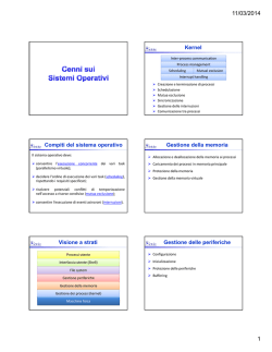
EDF optimality
Dertouzos Transformation
for (t = 0 to Dmax–1)
if (σ(t) ≠ E(t)) {
σ(tE) = σ(t);
σ(t) = E(t);
}
σ(t) = task executing at time t
⇒ nel senso della fattibilità [Dertouzos 1974]
E(t) = task with min d at time t
tE = time at which E is executed
Un algoritmo A è ottimo nel senso della
fattibilità se genera una schedulazione fattibile,
posto che
h ne esista
i
una.
τ1
τ2
τ3
Metodo dimostrativo
τ4
Basta dimostrare che, data una schedulazione
fattibile qualsiasi, la schedulazione generata da
EDF è anche fattibile.
0
2
Dertouzos Transformation
tE = time at which E is executed
σ ≠ σEDF
8
10
12
14
16
σ(t) = 3
E(t) = 2
tE = 7
16
Dertouzos Transformation
for (t = 0 to Dmax–1)
if (σ(t) ≠ E(t)) {
σ(tE) = σ(t);
σ(t) = E(t);
}
E(t) = task with min d at time t
6
t=5
13
σ(t) = task executing at time t
4
for (t = 0 to Dmax–1)
if (σ(t) ≠ E(t)) {
σ(tE) = σ(t);
σ(t) = E(t);
}
σ(t) = task executing at time t
E(t) = task with min d at time t
tE = time at which E is executed
τ1
τ1
τ2
τ2
τ3
τ3
τ4
τ4
0
2
4
6
8
10
12
14
16
σ(t) = 4
E(t) = 2
tE = 6
t=4
0
2
Dertouzos Transformation
tE = time at which E is executed
8
10
12
14
16
σ(t) = 3
E(t) = 2
tE = 7
17
Dertouzos Transformation
La trasformazione di Dertouzos preserva la schedulabilità,
infatti:
for (t = 0 to Dmax–1)
if (σ(t) ≠ E(t)) {
σ(tE) = σ(t);
σ(t) = E(t);
}
E(t) = task with min d at time t
6
t=5
14
σ(t) = task executing at time t
4
¾ ovvio per il pezzo che si anticipa!
¾ per il pezzo che si posticipa lo slack non può diminuire:
τ1
τ1
τ2
τ2
τ3
τ3
τ4
τ4
0
2
4
t=4
6
8
σ(t) = 4
E(t) = 2
tE = 6
10
12
14
16
0
15
2
4
6
t=5
8
10
12
14
16
18
3
12/03/2014
A property of optimal algoritms
Non Preemptive Scheduling
Il problema di trovare una schedulazione fattibile non
preemptive (noti i tempi di arrivo) è di tipo NP hard e può
essere risolto off-line mediante una ricerca di un albero:
Se un algoritmo ottimo (nel senso della
fattibilità) produce una schedulazione non
fattibile, allora nessun algoritmo può produrla.
empty schedule
depth = n
# leaves = n!
partial schedule
complexity: O(n n!)
Se un algoritmo A minimizza Lmax allora A è
anche ottimo nel senso della fattibilità. Non è
vero il viceversa.
N
F
N
N
N
N
F
N
complete schedule
19
22
Non Preemptive Scheduling
Bratley’s Algorithm
[Bratley 71]
( 1 | no-preem | Lmax )
Se si disabilita la preemption, EDF non è più ottimo:
Reduce la complessità media mediante pruning:
Feasible schedule
τ1
Si esplora un sottoalbero solo se la
schedulazione parziale è strongly feasible.
feasible
τ2
0
1
2
3
4
5
6
7
8
9
Una schedulazione parziale è strongly feasible
se rimane fattibile aggiungendo uno qualsiasi dei
task rimanenti.
EDF
τ1
τ2
0
1
2
3
4
5
6
7
8
9
20
23
Bratley’s Algorithm ( 1 | no-preem | Lmax )
Non Preemptive Scheduling
Per ottenere l'ottimalità in assenza di preemption
occorre essere chiaroveggenti, e decidere di lasciare la
CPU idle anche in presenza di task pronti:
τ1
1
2
3
4
5
6
7
8
Example
τ1
τ2
τ3
τ4
τ2
0
Riduce la complessità media per mezzo di pruning:
9
Se si impedisce si lasciare la CPU idle in presenza di
task pronti, allora EDF è ottimo.
NP-EDF è ottimo tra gli algoritmi di tipo
work conserving (non-idle algorithms)
ai
Ci
di
4
1
1
0
2
1
2
2
7
5
6
4
finishing time
6
6
τ2
Scheduled task
1
21
1
2
2
6
3
4
1
3
τ3
τ4
4
4
1
τ3
6
3
τ4
3
6
τ1
σ1 = {4, 2, 3, 1}
σ2 = {4, 3, 2, 1}
4
6
3
4
2
1
τ2
2
1
6
τ3
3
5
3
7
1
1
5
6
2
τ2
7
1
24
4
12/03/2014
Heuristic search
Heuristic algorithm
Spring algorithm [Stankovic & Ramamritham 87]
Spring algorithm [Stankovic & Ramamritham 87]
1. La schedulazione di N task è costruita in N passi
2. La ricerca è guidata da una funzione euristica H
Complexity:
3. Ad ogni passo, l'algoritmo seleziona il task che minimizza
la funzione euristica.
Backtracking
è possibile
min H
Exhaustive search:
O(N·N!)
Heuristic search:
O(N2)
Heuristic w. k btracks: O(kN2)
min H
min H
min H
min H
min H
min H
min H
25
28
Heuristic functions
Implementazione
Spring algorithm [Stankovic & Ramamritham 87]
Spring algorithm [Stankovic & Ramamritham 87]
Esempi di funzioni euristiche:
H = ri ⇒ FCFS
H = Ci ⇒ SJF
H = Di ⇒ DM
H = di ⇒ EDF
Se l'algoritmo non trova una schedulazione
fattibile, non è detto che questa non esista.
Se la schedulazione viene trovata, questa viene
memorizzata in una lista di disptach:
next
Funzioni euristiche composite:
∅
Task ID
H = w1 ri + w2 Di
H = w1 Ci + w2 di
H = w1 Vi + w2 di
start time
length
26
29
Heuristic algorithm
Spring algorithm [Stankovic & Ramamritham 87]
E' anche possibile gestire vincoli di precedenza:
Eligibility
τi
Ei = ∞
τi
Ei = 1
Funzioni euristiche:
H = Ei ( w1 ri + w2 Di )
H = Ei ( w1 Ci + w2 di )
27
5
12/03/2014
Problem formulation
τi (Ci, Ti)
Timeline Scheduling
job τik
Method
rik
• The time axis is divided in intervals of
equal length (time slots).
dik
• Each task is statically allocated in a slot in
order to meet the desired request rate.
For each periodic task, guarantee that:
• each job τik is activated at rik = (k−1)Ti
• The execution in each slot is activated by a
timer.
• each job τik completes within dik = rik + Di
31
34
Proportional share algorithm
Example
In each slot execute each task proportionally to Ui
Let: Ui = required feeding fraction
Δ = GCD (T1, T2) = 8
execute δi = UiΔ in each slot Δ
Pig
2
4/16
Cow
2
4
20/40
4
8
0
2
2
4
16
2
4
24
f
T
A
40 Hz
25 ms
B
20 Hz
50 ms
C
10 Hz
100 ms
task
2
T
Δ
4
32
0
40
25
50
NOTE: UiΔ ensures Ci in Ti, in fact: δi(Ti/Δ) = Ci
Feasibility test: Σδi ≤ Δ
i.e.
ΣUi ≤ 1
75
Guarantee:
100
125
150
175
200
CA + CB ≤ Δ
CA + CC ≤ Δ
32
Timeline Scheduling
(cyclic scheduling)
35
Implementation
It has been used for 30 years in military
systems, navigation, and monitoring systems,
and still used in critical control applications:
Examples
–
–
–
–
Δ = GCD (minor cycle)
T = lcm (major cycle)
Air traffic control
Space Shuttle
Boeing 777
Airbus
A
B
A
C
A
B
A
33
timer
minor
cycle
timer
timer
major
cycle
timer
36
6
12/03/2014
Timeline scheduling
Expandibility
Advantages
• Simple implementation (no real-time
operating
i system is
i required).
i d)
If one or more tasks need to be upgraded,
we may have to re-design the whole
schedule again.
Example: B is updated
• Low run-time overhead.
but
CA + CB > Δ
Δ
• It allows jitter control.
A
B
0
25
37
40
Expandibility
Timeline scheduling
• We have to split task B in two subtasks
(B1, B2) and re-build the schedule:
Disadvantages
• It is not robust during overloads.
A
• It is difficult to expand the schedule.
• It is not easy to handle aperiodic
activities.
0
B1
A
B2 C
25
A
50
Guarantee:
B1
A
B2
75
•••
100
CA + CB1 ≤ Δ
CA + CB2 + CC ≤ Δ
38
Problems during overloads
41
Expandibility
If the frequency of some task is changed,
the impact can be even more significant:
What do we do during task overruns?
• Let the task continue
– we can have a domino effect on all the other
tasks (timeline break)
• Abort the task
task
T
T
A
25 ms
25 ms
B
50 ms
40 ms
C
100 ms
100 ms
before
– the system can remain in inconsistent states.
39
minor cycle: Δ = 25
major cycle: T = 100
after
Δ=5
T = 200
40 sync.
per cycle!
42
7
12/03/2014
Example
How can we verify feasibility?
T
Δ
0
25
50
75
100
125
150
175
200
Δ
0
25
50
75
100
125
150
175
200
T
• Each task uses the processor for a fraction
of time:
C
Ui = i
Ti
• Hence the total processor utilization is:
n
C
Up = ∑ i
i =1 Ti
• Up is a misure of the processor load
43
46
Priority Scheduling
A necessary condition
Method
• Each task is assigned a priority based on its
timing constraints.
• We verify the feasibility of the schedule
using analytical techniques.
• Tasks are executed on a priority-based
kernel.
If Up > 1 the processor is overloaded
hence the task set cannot be schedulable.
However, there are cases in which Up < 1
but the task is not schedulable by RM.
44
Rate Monotonic (RM)
47
An unfeasible RM schedule
• Each task is assigned a fixed priority
proportional to its rate [Liu & Layland ‘73].
Up =
3
4
+
= 0.944
6
9
τA
0
25
50
75
τ1
100
τB
0
40
τC
0
0
3
6
9
0
3
6
9
12
15
18
12
15
18
τ2
80
deadline miss
100
45
48
8
12/03/2014
Utilization upper bound
U ub =
The least upper bound
Uub
3
3
+
= 0.833
6
9
1
τ1
0
3
6
9
12
15
18
0
3
6
9
12
15
18
Ulub
τ2
...
NOTE: If C1 or C2 is increased,
τ2 will miss its deadline!
Γ
49
52
A different upper bound
U ub =
A sufficient condition
2
4
+
= 0.9
4 10
If Up ≤ Ulub any task set is certainly
schedulable with the RM algorithm.
τ1
0
4
8
12
16
τ2
0
2
4
6
8
10
12
14
16
18
NOTE
20
If Ulub < Up ≤ 1 we cannot say anything
about the feasibility of that task set.
The upper bound Uub depends on the
specific task set.
50
53
A different upper bound
Rate Monotonic (RM)
• Each task is assigned a fixed priority
proportional to its rate [Liu & Layland ‘73].
2
4
+
= 1
4
8
U ub =
τA
τ1
0
4
8
12
16
0
4
8
12
16
0
25
50
75
100
τB
τ2
0
40
80
τC
The upper bound Uub depends on the
specific task set.
0
51
100
54
9
12/03/2014
Rate Monotonic is optimal
How to assign priorities?
• Typically, task priorities are assigned
based on the their relative importance.
RM is optimal among all fixed priority
algorithms (if Di = Ti):
If there exists a fixed priority assignment
which
hi h leads
l d to
t a feasible
f ibl schedule
h d l for
f Γ,
Γ then
th
the RM assignment is feasible for Γ.
• However, different priority assignments
can lead to different utilization bounds.
If Γ is not schedulable by RM, then it cannot
be scheduled by any fixed priority assignment.
55
Priority vs. importance
Deadline Monotonic is optimal
If τ2 is more important than τ1 and is assigned higher
priority, the schedule may not be feasible:
P1 > P2
58
If Di ≤ Ti then the optimal priority assignment is
given by Deadline Monotonic (DM):
τ1
DM
τ1
τ2
P2 > P1
τ2
RM
τ1
deadline miss
P2 > P1
τ1
P1 > P2
τ2
τ2
56
Priority vs. importance
But the utilization upper bound can be arbitrarily small:
If there exists a feasible schedule for Γ, then
EDF will
ill generate
t a feasible
f ibl schedule.
h d l
deadline miss
ε
τ1
EDF Optimality
EDF is optimal among all algorithms:
An application can be unfeasible even
when the processor is almost empty!
P2 > P1
59
∞
τ2
U =
ε
T1
+
C2
∞
If Γ is not schedulable by EDF, then it cannot
be scheduled by any algorithm.
0
57
60
10
12/03/2014
Identifying the worst case
EDF Example
Up =
Di = Ti
Feasibility may depend on the
initial activations (phases):
3
4
+
= 0.94
6
9
Up =
3
4
+
= 0.944
6
9
τ1
0
3
6
9
0
3
6
9
12
15
18
12
15
18
τ2
τ1
0
3
6
9
12
15
18
0
3
6
9
12
15
18
deadline miss
τ2
τ1
0
3
6
9
12
15
18
0
3
6
9
12
15
18
τ2
61
Critical Instant
The RM unfesible schedule
Up =
64
For any task τi, the longest response time occurs
when it arrives together with all higher priority tasks.
3
4
+
= 0.944
6
9
τ1
τ2
τ1
0
3
6
9
12
15
18
0
3
6
9
12
15
18
R2
τ2
τ1
τ2
deadline miss
R2
62
Critical Instant
Priority Assignments
For independent preemptive tasks under fixed priorities, the
critical instant of τi, occurs when it arrives together with all
higher priority tasks.
• Rate Monotonic (RM):
Pi ∝ 1/Ti
(static)
• Deadline Monotonic (DM):
Pi ∝ 1/Di
(static)
• Earliest Deadline First (EDF):
Pi ∝ 1/dik
(dynamic)
65
di,k = ri,k + Di
τ1
1/6
τ2
2/8
τ3
2/12
Idle time
τi
2/14
11
12/03/2014
Ulub for RM
Basic Assumptions
• In 1973, Liu and Layland proved that for a
set of n periodic tasks:
A1.
Ci is constant for every instance of ti
A2.
Ti is constant for every instance of ti
(
A3
A3.
F each
For
h task,
k Di = Ti
A4.
Tasks are independent:
)
RM
U lub
= n 21/ n − 1
for n → ∞
• no precedence relations
• no resource constraints
• no blocking on I/O operation
Ulub → ln 2
67
70
RM Schedulability
CPU%
100
90
80
70
60
50
40
30
20
10
0
69%
1
2
3
4
5
6
7
8
9
10
n
68
RM Guarantee Test
• We compute the processor utilization as:
n
C
Up = ∑ i
i =1 Ti
• Guarantee Test (only sufficient):
(
)
U p ≤ n 21/ n − 1
69
12
© Copyright 2026 Paperzz