INTRODUCTION TO THE FUNDAMENTAL GROUPS
2014 年前期理科大
MUTSUO OKA
1. 基本概念
1.1. Loops and Fundamental group. Let X be an arcwise connected topological
space. Consider the homotopy classes of loops starting at a fixed point b0 ∈ X :
Ω(X, b0 ). Recall that a loop is a continuous mapping σ : (I, ∂I) → (X, b0 ). Composition
σ ∗ τ of two loops σ, τ is defined as
σ(2t),
0 ≤ t ≤ 1/2
(σ ∗ τ )(t) =
τ (2t − 1), 1/2 ≤ t ≤ 1
Let c be the constant loop at b0 and σ −1 be the loop defined by σ −1 (t) = σ(1 − t).
Proposition 1.
(1) (Well-defined up-to homotopy) σ ≃ σ ′ , τ ≃ τ ′ =⇒ σ ∗ τ ≃
σ′ ∗ τ ′.
(2) (Associativity) σ ∗ (τ ∗ ω) ≃ (σ ∗ τ ) ∗ ω.
(3) (Unit element) σ ∗ c ≃ σ ≃ c ∗ σ.
(4) (Inverse) σ ∗ σ −1 ≃ σ −1 ∗ σ ≃ c.
In particular, Ω(X, b0 ) is a group.
We denote this group by π1 (X, b0 ).
Proposition 2. If (X, b0 ) ≃ (Y, y0 ), π1 (X, b0 ) ∼
= π1 (Y, y0 ).
Example 3. π1 (S 1 , b0 ) ∼
= Z. π1 (R2 \ {o}) ∼
= Z.
Proposition 4. b′0 ∈ X, ℓ : [0, 1] → X, ℓ(0) = b0 , ℓ(1) = b′0 .
ψ : π1 (X, b0 ) → π1 (X, b′0 ), ω → ℓ−1 ωℓ
は群の同型写像。
参考図書:田村一郎、岩波全書「トポロジー」小島 定吉:
「トポロジー入門」共立
1991 Mathematics Subject Classification. 14H30,14H45, 32S55.
Key words and phrases. θ-Alexander polynomial, fundamental group.
1
2
M. OKA
1.2. Hurewicz theorem.
Theorem 5. The canonical homomorphism π1 (X, b0 ) → H1 (X) is a surjective and the
kernel is the commutator subgroup of π1 (X, b0 ).
1.3. van Kampen Lemma. Assume we have groups G1 , G2 , G12 and group homomorphisms ϕ1 : G12 → G1 and ϕ2 : G12 → G2 . Then amalgamated product G1 ∗ G2 of
G12
G1 , G2 over G12 is the quotient group of the free product G1 ∗ G2 by the normal group
generated by the elements {ϕ1 (g)ϕ2 (g)−1 | g ∈ G12 }.
(1) If ϕ1 , ϕ2 are trivial homomorphisms, G1 ∗ G2 ∼
= G1 ∗ G2 .
G12
(2) If ϕ2 is a surjective, G1 ∗ G2 ∼
= G1 /N ϕ1 (Kerϕ2 ) where N H is the normal
Example 6.
G12
subgroup generated by H.
Suppose that X = X1 ∪ X2 and put X12 = X1 ∩ X2 . Assume that those subspaces
X12 , X1 , X2 are arcwise connected and b0 ∈ X12 .
Lemma 7. (van Kampen) The fundamental group π1 (X, b0 ) is isomorphic to
π1 (X1 )
∗
π1 (X2 ).
π1 (X12 ,b0 )
Lemma 8. (Homotopy invariance) Suppose that f : (X, b0 ) → (Y, c0 ) is a homotopy
equivalence. Then π1 (X, b0 ) ∼
= π1 (Y, c0 ).
Example 9. 1. π1 (P1 \ {k + 1points}) ∼
= F (k) where F (k) is a free group of rank k.
2
2. Show that a 2-simplex ∆ and a unit disk D = {(x, y) | x2 +y 2 ≤ 1} are homotopic.
1.4. Covering. Let π : (E, e0 ) → (X, b0 ) be a covering. The covering transformation
G(E/X) is the group of transformations φ : E → E such that π ◦ φ = π. The covering
is called normal (or Galois) if G(E/X) acts transitively to π −1 (b0 ).
Proposition 10.
(1) Let π : (E, e0 ) → (X, b0 ) is a covering. Then π♯ : π1 (E, e0 ) →
π1 (X, b0 ) is injective.
(2) It is normal iff π1 (E, e0 ) is a normal subgroup of π1 (X, b0 ). In this case, the
following is exact.
1 → π1 (E, e0 ) → π1 (X, b0 ) → G(E/X) → 1
証明:(1)π♯ is injective: If π(σ) ≃ c, there is a homotopy h : σ ◦ π ≃ c. This can be
˜ : I × I → E so that h|t = 0 = σ. Then h|t = 1 = c.
lifted to h
記号:E の道 ℓ の π による像を ℓ, B の道 ℓ に対し e ∈ π −1 (ℓ(0)) から始まる持ち上
げを ℓ˜e であらわす。
2) Suppose that π1 (E) is a normal subgroup. Take σ ∈ π1 (E, e0 ) and e ∈ π −1 (b0 ).
Then the lift of π♯ σ from e is also closed: (正規なことは基点を変えても同じに注意。)
INTRODUCTION TO THE FUNDAMENTAL GROUPS
3
(∵): Take a path ℓ from e0 to e. Then ℓσℓ−1 is conjugate to σ. So its lift is also
closed by the normality.
ℓσℓ−1 = ℓ˜
σe ℓ−1 σ˜e (1)
これは σ
˜e (1) = e を意味する。
a) ∀σ ∈ π1 (X), define ϕσ : E → E: x ∈ E, take a path ℓ from
ϕσ (x) to be the end point of the lift of (ℓ−1 σℓ)x :
0
to e0 to x and define
ϕσ (x) = ℓ−1 σ
˜e0 (ℓ)σ˜e0 (1) (1)
well-definedness: Suppose τ = ωσω −1 , ∃ω ∈ π1 (B, b0 ). Put
ξ := στ −1 = σωσ −1 ω −1 ∈ π1 (E, e0 )
で上からのループ。
((ℓ−1 σℓ)(ℓ−1 τ −1 ℓ))∼ = ℓ−1 στ −1 e0 ˜ℓe0 = ℓ−1 ξ˜x ℓ
でループ。すなわち σ, τ に依存すない。
b)Suppose that ℓ′ is another path from e0 to x. すると ω := ℓℓ′ −1 ∈ π1 (E, e0 ).
−1
−1
−1
ℓ−1 σℓ(ℓ′ σℓ′ )−1 = ℓ−1 σ(ℓℓ′ )σ −1 ℓ′ = ℓ′ ω −1 σωσ −1 ℓ′
is closed.
c) 逆に ψ ∈ G(E/X) をとる。ℓ を e0 から ψ(e0 ) への道を一つとれ。σ := π ◦ ℓ ∈
π1 (X, b0 ). ϕ を σ に対応する変換とすると、ϕ = ψ を示せ。
Proposition 11. Assume that a group G is acting to a space E freely and properly
discontinuously. Let X be the quotient space E/G. Then the canonical mapping π :
E → X is a normal covering.
”freely and properly discontinuously” とは任意の点 x ∈ E にたいし開近傍 U があっ
て、{gU |g ∈ G} が交わらないときをいう。
Example 12. 1. Let S 3 = {(z1 , z2 ) ∈ C2 | ∥z∥ = 1}. Let ζ := exp(2πi/p). Consider the
action
Z/pZ × S 3 → S 3 ,
(ζ a , (z1 , z2 )) = (z1 ζ a , z2 ζ a ).
The quotient space is called a Lens space L(p). We have π1 (L(P ) ∼
= Z/pZ.
1.5. Fibration. Assume that p : E → B is a locally trivial fibration with a connected
fiber F . Then we have the exact sequence:
· · · → π2 (B) → π1 (F ) → π1 (E) → π1 (B) → 1
4
M. OKA
Example 13. (Projective hypersurfaces are simply connected.) Let f (z) is a reduced
homogeneous polynomial of n + 1) variables and let K = f −1 (0) ∩ S 2n+1 . Then by
Milnor, K is (n − 2) -connected. Let V be the projective hypersurface in Pn . Thus if
n ≥ 3, K is simply connected. From the above exact sequence, we see that π1 (V ) = 1
and π2 (V ) surjects to Z for dim V ≥ 2.
2. Simplicial space
2.1. 複体の基本群. 田村一郎、「トポロジー」、岩波全書
K を複体とし、ai で頂点を表す。
頂点列 ℓ = (ai0 , . . . , aiq ) : が 折れ線 ⇐⇒
(i) [aij , aij+1 ] が1単体かまたは
(ii) aij = aij+1 .
ℓ の終点と ℓ′ の始点が同じなら合成 ℓ · ℓ′ が自然に定義出来る。同様に逆折れ線 ℓ−1
も定義出来る。閉折れ線とは終点と始点が同じ時をいう。
基本変形:
(I) (...ai ai ...) → (...ai ...)
(II) (...ai aj ai ...) → (...ai ...)
(III) (...ai aj ak ...) → (...ai ak ...) if (ai , aj , ak ): 2-simplex
有限回の基本変形で移りあうとき ℓ ≃ ℓ′ と書き、その同値類を [ℓ] とかく。
定義: π(K, a0 ): homotopy classes of closed path at a0 .
Theorem 14. 自然な準同型 ρ : π(K, a0 ) → π1 (|K|, a0 ) is bijective.
単体近似定理を使うので復習。
∪
2.2. 単体近似. 定義: a ∈ VertexK, OK (a) := a<σ Intσ.
∩
2. a0 , . . . , ar がある単体の頂点 ⇐⇒ ri=0 OK (ai ) ̸= ∅。
∀a (vertex), f (OK (a)) ⊂ OK ′ (φ(a)).
3. φ : K → K ′ が単体写像から、その幾何的位相空間の連続写像が引き起される:
φ¯ : |K| → |K ′ |.
定義:. f : |K| → |K ′ |, φ : K → K ′ が f の単体近似とは任意の頂点 a ∈ K に対し
て、f (OK (a)) ⊂ OK ′ (φ(a)).
Proposition 15. Let φ be a simplicial approximation of f . Then φ ≃ φ.
¯
の証明が意味を持つために次を証明せよ。
レポート問題 16.
∅.
(1) 頂点 a1 , . . . , ak がある単体の σ の頂点 ⇐⇒ ∩ki=1 OK (ai ) ̸=
INTRODUCTION TO THE FUNDAMENTAL GROUPS
5
(2) x ∈ Int(σ), σ = (a1 , . . . , ak ) とする. 命題の状況で
x ∈ ∩ki=1 OK (ai ) =⇒
f (x) ∈ f (∩ki=1 OK (ai )) ⊂ ∩ki=1 f (OK (ai )) ⊂ ∩ki=1 OK ′ (φ(ai )) ⊂ Int(φ(a1 ), . . . , φ(ak )).
Proposition 17. For f : |K| → |K ′ |, there exists n such that f (OK (Sdr (K), a)) ⊂
OK ′ (a′ ), ∃a′ for any r ≥ n. このとき単体写像 φ : K → K ′ があって、f は φ の単体
近似。
証明: a : vertex, ∃a′ , f (OSdn (K),a ) ⊂ OK ′ (a′ ). Define φ(a) = a′ .
前半の主張の証明は次の命題を示せ。
レポート問題 18. 単体 σ ∈ S に対し d(σ) をその直径。d(K) := max{d(σ)|σ ∈ S} で
定義する。K を m 次元複体とする時一回の重心細分で
m
d(Sd(K)) ≤
d(K).
m+1
を示せ。
定理 14 の証明:全射:ω : (I, ∂I) → (|K|, a0 ) をとる。f = ω, L = I とする。
∃n, ∀r ≥ n, f : |Sdr (L)| → |K| を単体近似とする単体写像が存在する:
φ : Sdr L → K
単射:K の閉じた折線 ℓ′ = (a0 , ai1 , . . . , ajq , a0 ),ω ′ = ρ(ℓ) とする。ω ′ ≃ c とする。ℓ¯′ ≃ ¯
0
′
2
by F : I × I → |K | なら ∃n, I × I を n の正方形に分けて正方形は対角線を加えて 2n2
三角形に分る。
f ([k/n, (k + 1)/n] × [j/n, (j + 1)/k]) ⊂ OK ′ (ajk )
と出来る。但し aj,n = a0 。F を単体写像 (k/n, j/n) → ajk で近似する。ψ : Sdn (I)2 →
K ′.
2.3. 自由群、群の表示. 階数 n の自由群とは x1 , . . . , xn を生成元として全てのげんは
w = xεi11 · · · xεikk , εj = ±1
とかけ
j−1
j+2
ij = ij+1 , εj + εj+1 = 0 =⇒ w ∼ w′ = xεi11 · · · xij−1
xj+1
· · · xεikk
ε
ε
この変換(簡約)を有限回おこなって長さ0の元になるとき自明と定めると自然に群とな
る。簡約が出来無い表現を簡約かされた表現という。任意の元は唯ひとつの簡約かされた
表現をもつ。このとき G = F (n) と表す。R1 , . . . , Rs を F (n) の単語として N (R1 , . . . , Rs )
を R1 , . . . , Rs とその共役元で生成された正規部分ぐんとする。商群 G = F (n)/N を
G =< x1 , . . . , xn | R1 , . . . , Rs >
とかいて G の関係式表現、R1 , . . . , Rs を関係式という。
G =< x1 , . . . , xn | R1 = · · · = Rs = e >
6
M. OKA
とかくことが多い。
例1。
< x1 | xk1 >∼
= Z/kZ
2.4. 自由積. G1 , G2 を群とする。G1 , G2 の自由積 G1 ∗ G2 とは
xi1 xi2 · · · xik | xi ∈ G1 − {e1 } or xi ∈ G2 − {e2 }/ ∼
上の表現で同じ Gj の元が続けてあれば
xij , xij+1 ∈ Gs =⇒ w ∼ xi1 . . . xj−1 (xij xij+1 )xij+2 · · · xik
と簡約する。特に
xij xij+1 = e =⇒ w ∼ xi1 . . . xij−1 xij+2 · · · xik
この同値るいの群を G1 ∗ G2 とかく。とくに
このような簡約を出来るかぎり行って簡約が出来無い表現にしたものが唯1つある。
このような元の全体に積を自明にいれて群としたもの。
例2。
Zp ∗ Zq =< x, y | xp = y q = e >
2.5. 単体複体の基本関係式. 各頂点 ai に a0 から折線で継いで固定する。それを ℓ[ai ] と
起く。ℓ[a0 ] = (a0 ).
1-単体全体を {τ1 , . . . , τs }. τi =< ai , a′i > のとき閉じた道
ℓ(< τi >) := ℓ[ai ]τi ℓ[a′i ]−1
を対応させる。これらを基底にとる. x1 , . . . , xs . すなわち xi = ℓ(ai )τi ℓ(a′i )−1 .
ℓ[ai ] = (a0 , . . . , ai ), ℓ[a′i ] = (a0 , . . . , a′i )
=⇒ xi = ℓ(< τi >) = (a0 , . . . , ai , ai , a′i , . . . , a0 )
これに変形(I)をして既約にしたものを (a0 , a1 , . . . , ap , a0 ) とすると、これらは基底で
かけて
ri = xi (xεi11 . . . xiqq )−1 , i = 1, . . . , s
ε
の関係式をえる。また2単体を σ1 , . . . , σt とするとたとえば σi = (ak1 ak2 ak3 ) なら
ℓ(< ak1 ak2 >)ℓ(< ak2 ak3 >)ℓ(< ak3 ak1 ) = 1 から関係式
ri′ = xεa1 xεb2 xεc3 = 1
をえる。
Theorem 19.
π(K, a0 ) ∼
= {x1 , . . . , xs | r1 , . . . , rs = r1′ = · · · = rt′ = e}
INTRODUCTION TO THE FUNDAMENTAL GROUPS
7
例:K = ∂∆2 , 頂点 {a0 , a1 , a2 }, 辺:τ0 =< a0 , a1 >, τ1 =< a1 , a2 >, τ2 =< a2 , a0 >.
ℓ[a1 ] = (a0 , a1 ), ℓ[a2 ] =< a0 , a1 , a2 >
x0 = (a0 , a0 , a1 , a0 ), x1 = (a0 , a1 , a1 , a2 , a2 , a1 , a0 ), x2 = (a0 , a1 , a2 , a2 , a0 , a0 )
r0 = x0 = (a0 , a1 , a0 ) = x0 x−1
⇐⇒ x0 = e
0
r1 = x1 = (a0 , a1 , a2 , a1 , a0 ) = x0 x1 x−1
⇐⇒ x1 = e
1
r2 = x2 = (a0 , a1 , a2 , a0 ) = x0 x1 x2 ⇐⇒ r2 = ∅
すなわち π(K, a0 ) ∼
=< x0 , x1 , x2 | x0 = x1 = e >∼
= Z.
2.5.1. ファンカンペン 多面体. K = K1 ∪K2 , K0 = K1 ∩K2 ,K0 , K1 , K2 は連結。a0 ∈ K0
にとる。ιi : K0 → Ki . このとき
Theorem 20. N を π(K1 , a0 ) ∗ π(K2 , a0 ) の正規部分群で
{ι1 (α)ι2 (α)−1 | α ∈ π(K0 , a0 )}
で生成されるものとする。このとき
π(K, a0 ) ∼
= π(K1 , a0 ) ∗ π(K2 ∗ a0 )/N.
証明:K0 の頂点:a0 , . . . , as0
K1 の頂点:a0 , . . . , as0 , b1 , . . . , bs0 +s1 ,
K2 の頂点:a0 , . . . , as0 , b′s0 +1 , . . . , b′s0 +s2 ,
ℓ(ai ) は K0 ないで選ぶ。
1-simplex: K0 : τ1 , . . . , τt0
K1 : τ1 , . . . , τt0 , τt0 +1 , . . . , τt0 +t1
K2 : τ1 , . . . , τt0 , τt′0 +t1 +1 , . . . , τt′0 +t1 +t2
2-simplex: K0 : σ1 , . . . , σp0
K1 : σ1 , . . . , σp0 , σp0 +1 , . . . , σp0 +p1
K2 : σ1 , . . . , σp0 , σp′ 0 +p1 +1 , . . . , σp′ 0 +p1 +p2
そうすると
π(K0 , a0 ) = ⟨x1 , . . . , xt0 |r1 , . . . , rt0 , r1′ , . . . , rp′ 0 ⟩
π(K1 , a0 ) = ⟨¯
x1 , . . . , x¯t0 , xt0 +1 . . . , xt0 +t1
|r1 , . . . , rt0 , . . . , rt0 +t1 , r1′ , . . . , rp′ 0 , . . . , rp′ 0 +p1 ⟩
π(K2 , a0 ) = ⟨¯
x′1 , . . . , x¯′t0 , xt0 +t1 +1 . . . , x¯t0 +t1 +t2
|r1 , . . . , rt0 , rt0 +t1 +1 . . . , rt0 +t1 +t2 , r1′ , . . . , rp′ 0 , rp′ 0 ,p1 +1 . . . , rp′ 0 +p1 ⟩
π(K, a0 ) = ⟨ˆ
x1 , . . . , xˆt0 , xˆt0 +t1 +1 . . . , xˆt0 +t1 +t2
|r1 , . . . , . . . , rt0 +t1 +t2 , r1′ , . . . , . . . , rp′ 0 +p1 ⟩
8
M. OKA
一方
ιi : xi → x¯i , or x¯′i
N : x¯i (¯
x′i )−1 , i ≤ t0
従って、π(K, a0 ) ∼
= π(K1, a0 ) ∗ π(K2 , a0 )/N .
1 章の練習問題 (レポート)
loop の合成に関して結合律 σ(τ ξ) ≃ στ )ξ を示せ。
loop の合成に関し σc ≃ cσ ≃ σ を示せ.
loop の合成に関して σσ −1 ≃ c を示せ.
基底点の取替えに関して ψ : π1 (X, b0 ) → π1 (X, b′0 ) が群の同型写像であることを
示せ。
(5) 被覆写像 p : E → X に対し、e0 ∈ E, b0 ∈ X を p(e0 ) = b0 にとる。p♯ :
π1 (E, e0 ) → π1 (X, b0 ) は単射であることを示せ。
(6) 被覆写像 p : E → X に対し、N := p♯ (π1 (E, e0 )) が正規部分群とする。g¯ ∈
π1 (X, b0 )/N に対し、g を持ち上げて g˜ : ([0, 1], 0) → (E, e0 )、e0 → g˜(1) を考え
れば、Ψ : π1 (X, b0 )/N → G(E/X) の同型写像となることを示せ。
(7) トーラス T := I 2 / ∼ を考える。I 2 の単体分割
(1)
(2)
(3)
(4)
a0
a1
c3
b2
b1
c1
a0
a1
a2
a0
c4
b2
c2
b1
a2
a0
Figure 1. トーラスの単体分割
(8)
(9)
(10)
(11)
を考える。1単体、2単体を全てあげよ。π(T, a0 ) をけいさんせよ。
穴のあいた円 Sn := {(x, y) ∈ R2 | x2 + y 2 = 1/2 + 1/n, x + yi ̸= exp(nπi/10)}
を考えて、X := R2 \ ∪∞
n=1 Sn とする。X は連結であることを示せ。X は弧状連
結でないことを示せ。(ひんと:O と (1, 0) は道でつなげないことを示せ。
R2 \ {(0, 0)} は S 1 = {(x, y)|x2 + y 2 = 1} に変位レトラクトすることを示せ。
弧状連結な位相空間 X, Y に対し、x0 ∈ X, y0 ∈ Y を固定する。π1 (X × Y ) ∼
=
π1 (X, x0 ) × π1 (Y, y0 ) を示せ。
一点和 X ∨ Y を X ⨿ Y /x0 = y0 で定義する。S 1 ∨ S 1 の基本群を求めよ。
INTRODUCTION TO THE FUNDAMENTAL GROUPS
9
(12) T \ {(1/2, 1/2)} は S 1 ∨ S 1 とホモトーピックなることを示せ。
(13) Xn を R2 から n 点除いた空間とする。X2 ≃ S 1 ∨ S 1 を示せ。同様に Xn ≃
S 1 ∨ · · · ∨ S 1 (n個) を示せ。
(14) π1 (R3 − {onepoint}) = 1 を示せ。
(15) X を 地球野表面に南極と北極をつないだ直線を合わせた空間とする:
X := {(x, y, z) ∈ R3 | x2 + y 2 + z 2 = 1} ∪ {(0, 0, z) | − 1 ≤ z ≤ 1}.
この時 π1 (X) ≃ Z を示せ。
10
M. OKA
3. 射影曲線の補空間の基本群
The rest of lectures are mainly based on my lecture: Oka, Mutsuo A survey on Alexander polynomials of plane curves. Singularits Franco-Japonaises, 209―232, S´emin.
Congr., 10, Soc. Math. France, Paris, 2005.
3.1. Introduction. For a given hypersurface V ⊂ Pn , the fundamental group π1 (Pn −
V ) plays a crucial role when we study geometrical objects over Pn which are branched
over V . By the hyperplane section theorem of Zariski [59], Hamm-Lˆe [19],
Theorem 21. (Hamm-Le,[19]) The fundamental group π1 (Pn − V ) is isomorphic to the
fundamental group π1 (P2 − C) where P2 is a generic projective subspace of dimension
2 and C = V ∩ P2 .
A systematic study of the fundamental group was started by Zariski [58] and further
developments have been made by many authors. See for example Zariski [58], Oka
[33] ∼ [35], Libgober [24]. For a given plane curve, the fundamental group π1 (P2 −
C) is a strong invariant but it is not easy to compute. Another invariant which is
weaker but easier to compute is the Alexander polynomial ∆C (t). This is related
to a certain infinite cyclic covering space branched over C. Important contributions
are done by Libgober, Randell, Artal, Loeser-Vaqui´e, and so on. See for example
[22, 16, 48, 28, 52, 13, 10, 46, 31, 1, 17, 26, 49, 2, 51, 8]
3.2. Fundamental groups.
3.2.1. van Kampen Pencil method. Let C ⊂ P2 be a projective curve which is defined
by C = {[X, Y, Z] ∈ P2 | F (X, Y, Z) = 0} where F (X, Y, Z) is a reduced homogeneous
polynomial F (X, Y, Z) of degree d. We assume that B0 ∈
/ C. We consider Pencil of
lines passing through B0 . For simplify, we assume that B0 = (0 : 1 : 0) and pencil lines
are Lη : x = η (X = ηZ).
Lτ is called a generic line of the pencil for C if Lτ and C meet transversally. If Lτ
is not generic, either Lτ passes through a singular point of C or Lτ is tangent to C at
some smooth point. We fix two generic lines Lτ0 and L∞ = {Z = 0}.
We denote the affine line Lτ − {B0 } by Laτ . Note that Laτ ∼
= C. The complement
a
a
2
Lτ0 − Lτ0 ∩ C (resp. Lτ0 − Lτ0 ∩ C) is topologically S minus d points (resp. (d + 1)
points). We take b0 = B0 as the base point in the case of π1 (P2 − C). In the affine
case π1 (C2 − C), we take the base point b0 on Lτ0 which is sufficiently near to B0 but
b0 ̸= B0 .
Let us consider two free groups
F1 = π1 (Lτ0 − Lτ0 ∩ C, b0 ) and
of rank d − 1 and d respectively.
F2 = π1 (Laτ0 − Laτ0 ∩ C, b0 ).
INTRODUCTION TO THE FUNDAMENTAL GROUPS
11
We consider the set Σ := {τ ∈ P1 | Lτ is a non-generic line} ∪ {∞}.
Thus there exists canonical action of π1 (P1 − Σ, τ0 ) on F1 and F2 . We call this action
the monodromy action of π1 (P1 − Σ, τ0 ). For σ ∈ π1 (P1 − Σ, τ0 ) and g ∈ F1 or F2 , we
denote the action of σ on g by g σ . The relations in the group Fν
(R1 )
⟨g −1 g σ = e | g ∈ Fν , σ ∈ π1 (P1 − Σ, τ0 )⟩,
ν = 1, 2
are called the monodromy relations.
The normal subgroup of Fν , ν = 1, 2 which
are normally generated by the elements {g −1 g σ , | g ∈ Fν } are called the groups of the
monodromy relations and we denote them by Nν for ν = 1, 2 respectively. The original
van Kampen Theorem can be stated as follows. See also [7, 6].
Theorem 22. ([55]) The following canonical sequences are exact.
1 → N1 → π1 (Lτ0 − Lτ0 ∩ C, b0 ) → π1 (P2 − C, b0 ) → 1
1 → N2 → π1 (Laτ0 − Laτ0 ∩ C, b0 ) → π1 (C2 − C, b0 ) → 1
Here 1 is the trivial group. Thus the fundamental groups π1 (P2 − C, b0 ) and π1 (C2 −
C, b0 ) are isomorphic to the quotient groups F1 /N1 and F2 /N2 respectively.
For a group G, we denote the commutator subgroup of G by D(G). The relation of
the fundamental groups π1 (P2 −C, b0 ) and π1 (C2 −C, b0 ) are described by the following.
Let ι : C2 − C → P2 − C be the inclusion map.
Lemma 23. ([32]) Assume that L∞ is generic.
(1) We have the following central extension.
γ
ι♯
1 → Z−→π1 (C2 − C, b0 )−→π1 (P2 − C, b0 ) → 1
A generator of the kernel Ker ι♯ of ι♯ is given by a lasso ω for L∞ .
(2) Furthermore, their commutator subgroups coincide i.e., D(π1 (C2 −C)) = D(π1 (P2 −
C)). In particular, π1 (P2 − C) is abelian off π1 (C2 − C) is abelian.
Proof. A loop ω is called a lasso for an irreducible curve D if ω is homotopic to
a path written as ℓ ◦ τ ◦ ℓ−1 where τ is the boundary positively oriented circle of a
normal small disk of D at a smooth point and ℓ is a path connecting the base point.
For the assertion (1), see [32]. We only prove the second assertion. Assume that C has
r irreducible components of degree d1 , . . . , dr . The restriction of the homomorphism ι♯
gives a surjective morphism ι♯ : D(π1 (C2 − C)) → D(π1 (P2 − C)). The generator τ
of the kernel Z is a lasso going around L∞ and it goes to d1 [C1 ] + · · · + dr [Cr ]. Thus
ker ι♯ ∩ D(π1 (C2 − C)) = {1}.
12
M. OKA
3.3. Examples of monodromy relations. (I) Tangent relation. Assume that C
and L0 intersect at a simple point P with intersection multiplicity p. Such a point is
called a flex point of order p − 2 if p ≥ 3 ([58]). This corresponds to the case q = 1.
Then the monodromy relation gives ξ0 = ξ1 = · · · = ξp−1 and thus π1 (C2 − C) ∼
= Z.
ξ2
ξ1
ξ0
Figure 2. Local Generators
As a corollary, Zariski proves that the fundamental group π1 (P2 − C) is abelian if
C has a flex of order ≥ d − 3. In fact, if C has a flex of order at least d − 3, the
monodromy relation is given by ξ0 = · · · = ξd−2 . On the other hand, we have one
more relation ξd−1 . . . ξ0 = e. In particular, considering the smooth curve defined by
C0 = {X d − Y d = Z d }, we get that π1 (P2 − C) is abelian for a smooth plane curve C,
as C can be joined to C0 by a path in the space of smooth curves of degree d.
(II) Nodal relation. Assume that C has an ordinary double point (i.e., a node) at
the origin and assume that C is defined by x2 − y 2 = 0 near the origin. This is the case
when p = q = 2. Then as the monodromy relation, we get the commuting relation:
ξ1 ξ2 = ξ2 ξ1 . Assume that C has only nodes as singularities. The commutativity of
π1 (P2 − C) was first asserted by Zariski [58] and is proved by Fulton-Deligne [14, 18].
See also [30, 46, 45].
(III) Cuspidal relation. Assume that C has a cusp at the origin which is locally
defined by y 2 − x3 = 0 (p = 2, q = 3). Then monodromy relation is: ξ1 ξ2 ξ1 = ξ2 ξ1 ξ2 .
This relation is known as the generating relation of the braid group B3 (Artin [4]).
Similarly in the case p = 3, q = 2, we get the relation ξ1 = ξ3 , ξ1 ξ2 ξ1 = ξ2 ξ1 ξ2 .
3.4. First Homology. Let X be a path-connected topological space. By the theorem
of Hurewicz, H1 (X, Z) is isomorphic to the the quotient group of π1 (X) by the commutator subgroup (see [50]). Now assume that C is a projective curve with r irreducible
components C1 , . . . , Cr of degree d1 , . . . , dr respectively. By Lefschetz duality, we have
the following.
INTRODUCTION TO THE FUNDAMENTAL GROUPS
13
Proposition 24. H1 (P2 −C, Z) is isomorphic to Zr−1 ×(Z/d0 Z) where d0 = gcd(d1 , . . . , dr ).
In particular, if C is irreducible (r = 1), the fundamental group is a cyclic group of
order d1 .
3.5. Generic cuspidal relation. We consider a model curve Cp,q which is defined by
y p − xq = 0 and we study π1 (C2 − Cp,q ). For this purpose, we consider the pencil lines
x = t, t ∈ C. We consider the local monodromy relations for σ, which is represented by
the loop x = ε(2πit), 0 ≤ t ≤ 1. We take local generators ξ0 , ξ1 , . . . , ξp−1 of π1 (Lε , b0 ))
as in Figure 2. Every loops are counter-clockwise oriented. It is easy to see that each
point of Cp,q ∩ Lε are rotated by the angle 2π × q/p. Let q = mp + q ′ , 0 ≤ q ′ < p. Then
the monodromy relations are:
ω m ξ ′ ω −m , 0 ≤ j < p − q ′
j+q
(R1 )
ξj (= ξjσ ) =
ω m+1 ξj+q′ −p ω −(m+1) , p − q ′ ≤ j ≤ p − 1
(R2 )
ω = ξp−1 · · · ξ0 .
3.5.1. Typical groups. For the convenience, we introduce two groups G(p, q) and G(p, q, r).
G(p, q) := ⟨ξ1 , . . . , ξp , ω | R1 , R2 ⟩,
G(p, q, r) := ⟨ξ1 , . . . , ξp , ω | R1 , R2 , R3 ⟩
where R3 is the vanishing relation of the big circle ∂DR = {|y| = R}:
(R3 )
ω r = e.
Now the above computation gives the following.
Lemma 25. We have π1 (C2 − Cp,q , b0 ) ∼
= G(p, q) and if p ≥ q, π1 (P2 − Cp,q , b0 ) ∼
=
G(p, q, 1).
Note that and G(p, q, 1) = Z/pZ. The groups of G(p, q) and G(p, q, r) are studied in
[34, 15]. For instance, we have
Theorem 26. ([34]) (i) Let s = gcd(p, q), p1 = p/s, q1 = q/s. Then ω q1 is the center
of G(p, q).
(ii) Put a = gcd(q1 , r). Then ω a is in the center of G(p, q, r) and has order r/a and the
quotient group G(p, q, r)/ < ω a > is isomorphic to Zp/s ∗ Za ∗ F (s − 1).
Corollary 27. ([34]) Assume that r = q. Then G(p, q, q) = Zp1 ∗ Zq1 ∗ F (s − 1). In
particular, if gcd(p, q) = 1, G(p, q, q) ∼
= Zp ∗ Zq . Let us recall some useful relations which follow from the above model.
14
M. OKA
3.6. Relation with Milnor Fibration. Let F (X, Y, Z) be a reduced homogeneous
polynomial of degree d which defines C ⊂ P2 . We consider the Milnor fibration of F
[27] F : C3 − F −1 (0) → C∗ and let M = F −1 (1) be the Milnor fiber. By the theorem of
Kato-Matsumoto [21], M is path-connected. We consider the following diagram where
the vertical map is the restriction of the Hopf fibration.
C∗
i
M
ι
j
↘
→ C3 − F −1 (0) −→ C∗
p
q
↘
F
P2 − C
Proposition 28. ([32])(I) The following conditions are equivalent.
(i) π1 (P2 − C) is abelian.
(ii) π1 (C3 − F −1 (0)) is abelian.
(iii) π1 (M ) is abelian and the first monodromy of the Milnor fibration h∗ : H1 (M ) →
H1 (M ) is trivial.
(II) Assume that C is irreducible. Then π1 (M ) is isomorphic to the commutator subgroup of π1 (P2 − C). In particular, π1 (P2 − C) is abelian if and only if M is simply
connected.
3.7. Degenerations and fundamental groups. Let C be a reduced plane curve.
The total Milnor number µ(C) is defined by the sum of the local Milnor numbers
µ(C, P ) at singular points P ∈ C. We consider an analytic family of reduced projective
curves Ct = {Ft (X, Y, Z) = 0}, t ∈ U where U is a connected open set with 0 ∈ C
and Ft (X, Y, Z) is a homogeneous polynomial of degree d for any t. We assume that
Ct , t ̸= 0 have the same configuration of singularities so that they are topologically
equivalent but C0 obtain a bigger total Milnor number, i.e., µtot (Ct ) < µtot (C0 ). We call
such a family a degeneration of Ct at t = 0 and we denote this, for brevity, as Ct → C0 .
Then we have the following property about the fundamental groups.
Theorem 29. There is a canonical surjective homomorphism for t ̸= 0: φ : π1 (P2 −
C0 ) → π1 (P2 − Ct ). In particular, if π1 (P2 − C0 ) is abelian, so is π1 (P2 − Ct ).
Proof. Take a generic line L which cuts C0 transversely. Let N be a neighborhood of
C0 so that ι : P2 − N → P2 − C0 is a homotopy equivalence. For instance, N can be a
regular neighborhood of C0 with respect to a triangulation of (P2 , C0 ). Take sufficiently
small t ̸= 0 so that Ct ⊂ N . Then taking a common base point at the base point of the
pencil, we define φ as the composition:
ι−1
#
π1 (P − C0 , b0 )−→π1 (P2 − N, b0 ) → π1 (P2 − Ct , b0 )
2
INTRODUCTION TO THE FUNDAMENTAL GROUPS
15
We can assume that Ct and L intersect transversely for any t ≤ ε and L − L ∩ N →
L − L ∩ Ct is a homotopy equivalence for 0 ≤ t ≤ ε. Then the surjectivity of φ follows
from the following commutative diagram
β′
α′
π1 (L − L∩ C0 , b0 ) ←− π1 (L − L ∩ N, b0 ) −→ π1 (L − L∩ Ct , b0 )
a
c
b
π1 (P2 − C0 , b0 )
α
←−
π1 (P2 − N, b0 )
β
−→
π1 (P2 − Ct , b0 )
where the vertical homomorphisms a, c are surjective by Theorem 22 and α, α′ , β ′ are
canonically bijective. Thus β is also surjective. Thus define φ : π1 (P2 − C0 , b0 ) →
π1 (P2 − Ct , b0 ) by the composition α−1 ◦ β. The second assertion is immediate from the
first assertion. This completes the proof.
Applying Theorem 29 to the degeneration Ct ∪ L → C0 ∪ L, we get
Corollary 30. There is a a surjective homomorphism: π1 (C2 − C0 ) → π1 (C2 − Ct ).
Corollary 31. Let Ct , t ∈ C be a degeneration family. Assume that we have a presentation
π1 (P2 − C0 ) ∼
= ⟨g1 , . . . , gd | R1 , . . . , Rs ⟩
Then π1 (P2 − Ct ), t ̸= 0 can be presented by adding a finite number of other relations.
Corollary 32. (Sandwich isomorphism) Assume that we have two degeneration families
Ct → C0 and Ds → D0 such that D1 = C0 . Assume that the composition
π1 (P2 − D0 ) → π1 (P2 − Ds ) = π1 (P2 − C0 ) → π1 (P2 − Ct )
is an isomorphism. Then we have isomorphisms π1 (P2 − D0 ) ∼
= π1 (P2 − Dt ) and
π1 (P2 − C0 ) ∼
= π1 (P2 − Ct ).
Example 33. Assume that C is a reduced curve of degree d with n nodes as singularities
()
with n < d2 . By a result of J. Harris [20], there is a degeneration Ct of C = C1 so that
C0 obtains more nodes and C0 has no other singularities. (This was asserted by Severi
but his proof had a gap.) Repeating this type of degenerations, one can deform a given
()
nodal curve C to a reduced curve C0 with d2 nodes, which is a union of d generic lines.
On the other hand, π1 (P2 − C0 ) is abelian by Corollary 36 below. Thus we have
Theorem 34. ([58, 14, 20, 30, 46]) Let C be a nodal curve. Then π1 (P2 −C) is abelian.
3.8. Product formula. Assume that C1 and C2 are reduced curves of degree d1 and
d2 respectively which intersect transversely and let C := C1 ∪ C2 . We take a generic
line L∞ for C and we consider the the corresponding affine space C2 = P2 − L∞ .
Theorem 35. (Oka-Sakamoto [44]) Let φk : C2 −C → C2 −Ci , k = 1, 2 be the inclusion
maps. Then the homomorphism φ1# × φ2# : π1 (C2 − C) → π1 (C2 − C1 ) × π1 (C2 − C2 )
is isomorphic.
16
M. OKA
Corollary 36. Assume that C1 , . . . , Cr are the irreducible components of C and π1 (P2 −
Cj ) is abelian for each j and they intersect transversely so that Ci ∩ Cj ∩ Ck = ∅ for
any distinct three i, j, k. Then π1 (P2 − C) is abelian.
3.9. Zariski Pair. Let C, C ′ be a pair of plane curves. The pair is called a Zariski pair
if
(1) deg C = deg C ′ .
(2) There exist regular neighborhoods N and N ′ of C and C ′ and a homeomorphism
ψ : (N, C) → (N ′ , C ′ ) in which singular points of C are bijectively mapped to
singular points of C ′ .
(3) The pair (P2 , C) and (P2 , C ′ are not homeomorphic.
First example is found by Zariski in [58]. It is a pair of irreducible sextics with 6
cusps (C, C ′ where C is a so-called of torus type and its defining polynomial is written
as f (x, y) = f2 (x, y)3 + f3 (x, y)2 with deg fi = iand π1 (P2 − C) ∼
= Z2 ∗ Z3 . On the
other hand, there are no conic which contains 6 cusps of C ′ and Zariski proved that
π1 (P2 − C ′ is not isomorphic to Z2 ∗ Z3 . In [35], we gave a first explicit example of
such septic C ′ and proved that π1 (P2 − C ′ ) ∼
= Z6 . In [12], A. Degtyarev showed that
the moduli of such sextics is irreducible which implies that any non-torus sextics with
6 cusps has Z6 as the fundamental group. There are many Zariski pairs are found after
Zariski. Main tool for distinguish the topology of the complements of the curve is the
fundamental group π1 (P2 − C) or Alexander polynomial ∆C (t) which is defined later
[39, 40, 41, 3, 11, 12]. There are also a method of the existence or non-existence of a
dihedral cover by Tokunaga [53, 54].
3.10. Covering transformation. Assume that C is a reduced curve defined by f (x, y) =
0 in the affine space C2 := P2 − L∞ . The line at infinity L∞ is assumed to be generic
so that we can write
f (x, y) =
d
∏
(y − αi x) + (lower terms), α1 , . . . , αd ∈ C∗ , αj ̸= αk , j ̸= k.
i=1
Take positive integers n ≥ m ≥ 1. We assume that the origin O is not on C and
the coordinate axes x = 0 and y = 0 intersect C transversely and C ∩ {x = 0} and
C ∩ {y = 0} has no point on L∞ . Consider the doubly branched cyclic covering
Φm,n : C2 → C2 , (x, y) → (xm , y n ).
Put fm,n (x, y) := f (xm , y n ) and put Cm,n = {fm,n (x, y) = 0} = Φ−1
m,n (C). The topology
of the complement of Cm,n (C) depends only on C and m, n. We will call Cm,n (C) as a
generic (m, n)-fold covering transform of C.
INTRODUCTION TO THE FUNDAMENTAL GROUPS
17
If n > m, Cm,n (C) has one singularity at ρ∞ = [1; 0; 0] and the local equation at ρ∞
takes the following form:
d
∏
(ζ n − αi ξ n−m ) + (higher terms),
ζ = Y /X, ξ = Z/X
i=1
In the case m = n, we have no singularity at infinity. We denote the canonical
homomorphism (Φm,n )♯ : π1 (C2 − Cm,n (C)) → π1 (C2 − C) by ϕm,n for simplicity.
Theorem 37. ([36]) Assume that n ≥ m ≥ 1 and let Cm,n (C) be as above. Then the
canonical homomorphism
ϕm,n : π1 (C2 − Cm,n (C)) → π1 (C2 − C)
is an isomorphism and it induces a central extension of groups
ι
ϕm,n
1 → Z/nZ−→π1 (P2 − Cm,n (C))−→π1 (P2 − C) → 1
The kernel of ϕm,n is generated by an element ω ′ in the center and ϕm,n (ω ′ ) is homotopic
to a lasso ω for L∞ in the target space. The restriction of ϕm,n gives an isomorphism
of the respective commutator groups ϕm,n ♯ : D(π1 (P2 − Cm,n (C))) → D(π1 (P2 − C)).
We have also the exact sequence for the first homology groups:
Φm,n
1 → Z/nZ → H1 (P2 − Cm,n (C)) −→ H1 (P2 − C) → 1
Corollary 38. (1) π1 (P2 − Cm,n (C)) is abelian if and only if π1 (P2 − C) is abelian.
(2) Assume that C is irreducible. Put
F (x, y, z) = z d f (x/z, y/z),
Fm,n (x, y, z) = z dn fm,n (x/z, y/z)
Let Mm,n and M be the Minor fibers of Fm,n and F respectively. Then we have an
isomorphism of the respective fundamental groups: π1 (Mm,n ) ∼
= π1 (M ).
For a group G, we consider the following condition : Z(G) ∩ D(G) = {e} where Z(G)
is the center of G. This is equivalent to the injectivity of the composition: Z(G) →
G → H1 (G). When this condition is satisfied, we say that G satisfies homological
injectivity condition of the center (or (H.I.C)-condition in short). A pair of reduced
plane curves of a same degree {C, C ′ } is called a Zariski pair if there is an bijection
α : Σ(C) → Σ(C ′ ) of their singular points so that the two germs (C, P ), (C ′ , α(P ))
are topologically equivalent for each P ∈ Σ(C) and the fundamental group of the
complement π1 (P2 − C) and π1 (P2 − C ′ ) are not isomorphic. (This definition is slightly
stronger than that in [36].)
Corollary 39. ([36]) Let {C, C ′ } be a Zariski pair and assume that π1 (P2 −C ′ ) satisfies
(H.I.C)-condition. Then for any n ≥ m ≥ 1, {Cm,n (C), Cm,n (C ′ )} is a Zariski pair.
See also Shimada [49].
18
M. OKA
3.11. Non-generic covering. Let C be a given affine curve defined by f (x, y) = 0.
The covering ψn : C2 → C2 , (x, y) → (x, y n ) is more interesting for the purpose of
constructing a new curve with more singularities. Suppose that the line y = 0 is not
∏
generic with respect to C and assume that f (x, 0) = sj=1 (x − αj )νi . We assume that
C is non-singular on these points (αj , 0) and assume that {Pk | k = 1, . . . , t} are the
singular points of C. Then the pull-back Cn : f (x, y n ) = 0 contains the following
singularities.
• On C2 − {y = 0}, each singular point Pk produce n isomorphic singuarities on
Cn .
• On y = 0, the point (αj , 0) ∈ C produce a singular point which is locally written
as v n − uνj = 0 if νj ≥ 2.
Consider the following curve C defined by f (x, y) = 0.
(
)
(
)
f (x, y) = x2 (x − 1)2 x2 + 2 x −x2 (x − 1)2 (y − 1)+1/3 x2 − 1 (y − 1)2 −1/27 (y − 1)3
Its graph is as Figure 3.
Figure 3. Graph of C
√
The curve as two flex points at (± 2/3, 0). Let C2 be the double cover f (x, y 2 ) = 0.
It has six cusps and they are not on any single conic.
INTRODUCTION TO THE FUNDAMENTAL GROUPS
Figure 4. Graph of C2
19
20
M. OKA
4. Lecture 3
4.1. Alexander polynomial. Let X be a topological space which has a homotopy
type of a finite CW-complex and assume that we have a surjective homomorphism:
ϕ : π1 (X) → Z. Let t be a generator of Z and put Λ = C[t, t−1 ]. Note that Λ is
a principal ideal domain. Consider an infinite cyclic covering p : X → X such that
p# (π1 (X)) = Ker ϕ. Then H1 (X, C) has a structure of Λ-module where t acts as the
canonical covering transformation. Thus we have an identification:
H1 (X, C) ∼
= Λ/λ1 ⊕ · · · ⊕ Λ/λn
as Λ-modules. We normalize the denominators so that λi is a polynomial in t with
λi (0) ̸= 0 for each i = 1, . . . , n. The Alexander polynomial ∆(t) is defined by the
∏
product ni=1 λi (t).
The classical one is the case X = S 3 − K where K is a knot. As H1 (S 3 − K) = Z, we
have a canonical surjective homomorphism ϕ : π1 (S 3 − K) → H1 (S 3 − K, Z) induced by
the Hurewicz homomorphism. The corresponding Alexander polynomial is called the
Alexander polynomial of the knot K.
In our situation, we consider a plane curve C defined by a homogeneous polynomial
F (X, Y, Z) of degree d. Unless otherwise stated, we always assume that the line at
infinity L∞ is generic for C and we identify the complement P2 − L∞ with C2 . Let
ϕ : π1 (C2 − C) → Z be the canonical homomorphism induced by the composition
π1 (C2 − C)−→H1 (C2 − C, Z) ∼
= Zr −→Z
ξ
s
∑
where ξ is the Hurewicz homomorphism and s is defined by s(a1 , . . . , ar ) = ri=1 ai and r
is the number of irreducible components of C. We call s the summation homomorphism.
˜ → C2 − C be the infinite cyclic covering corresponding to Ker ϕ. The correLet X
sponding Alexander polynomial is called the generic Alexander polynomial of C and we
denote it by ∆C (t) or simply ∆(t) if no ambiguity is likely. It does not depend on the
choice of the generic line at infinity L∞ . Let M = F −1 (1) ⊂ C3 be the Milnor fiber of
F . The monodromy map h : M → M is defined by the coordinatewise multiplication
of exp(2πi/d). Randell showed in [48] the following important theorem.
Theorem 40. The Alexander polynomial ∆(t) is equal to the characteristic polynomial
of the monodromy h∗ : H1 (M ) → H1 (M ). Thus the degree of ∆(t) is equal to the first
Betti number b1 (M ).
Lemma 41. Assume that C has r irreducible components. Then the multiplicity of the
factor (t − 1) in ∆(t) is r − 1.
Proof. As hd = idM , the monodromy map h∗ : H1 (M ) → H1 (M ) has a period d.
This implies that h∗ can be diagonalized. Assume that ρ is the multiplicity of (t − 1)
INTRODUCTION TO THE FUNDAMENTAL GROUPS
21
in ∆(t). Consider the Wang sequence:
h −id
∗
H1 (M ) −→
H1 (M ) → H1 (E) → H0 (M ) → 0
where E := S 5 − V ∩ S 5 and V = F −1 (0). Then we get b1 (E) = ρ + 1. On the other
hand, by Alexander duality, we have H1 (E) ∼
= H 3 (S 5 , V ∩ S 5 ) and b1 (E) = r. Thus we
conclude that ρ = r − 1.
The following Lemma describes the relation between the generic Alexander polynomial and local singularities.
Lemma 42. (Libgober [22]) Let P1 , . . . , Pk be the singular points of C and let ∆i (t)
be the characteristic polynomial of the Milnor fibration of the germ (C, Pi ). Then the
∏
generic Alexander polynomial ∆(t) divides the product ki=1 ∆i (t)
Lemma 43. (Libgober [22]) Let d be the degree of C. Then the Alexander polynomial
∆(t) divides the Alexander polynomial at infinity ∆∞ (t) which is given by (td −1)d−2 (t−
1). In particular, the roots of Alexander polynomial are d-th roots of unity.
The last assertion also follows from Theorem 40 and the periodicity of the monodromy.
4.2. Fox calculus. Suppose that ϕ : π1 (X) → Z is a given surjective homomorphism.
Assume that π1 (X) has a finite presentation as
π1 (X) ∼
= ⟨x1 , . . . , xn | R1 , . . . , Rm ⟩
where Ri is a word of x1 , . . . , xn . Thus we have a surjective homomorphism ψ : F (n) →
π1 (X) where F (n) is a free group of rank n, generated by x1 , . . . , xn . Consider the
group ring of F (n) with C-coefficients C[F (n)]. The Fox differential
∂
: C[F (n)] → C[F (n)]
∂xj
is C-linear map which is characterized by the property
∂
xi = δi,j ,
∂xj
∂
∂u
∂v
(uv) =
+u
, u, v ∈ C[F (n)]
∂xj
∂xj
∂xj
The composition ϕ ◦ ψ : F (n) → Z gives a ring homomorphism γ : C[F (n)] → C[t, t−1 ].
The Alexander matrix A is m × n matrix with coefficients in C[t, t−1 ] and its (i, j)i
component is given by γ( ∂R
). Then it is known that the Alexander polynomial ∆(t)
∂xj
is given by the greatest common divisor of (n − 1)-minors of A ([9]). The following
formula will be useful.
∂ k
∂
∂ −k
∂ k
ω = (1 + ω + · · · + ω k−1 )
ω,
ω = −ω −k
ω
∂xj
∂xj
∂xj
∂xj
22
M. OKA
Example 44. We gives several examples.
1. Consider the trivial case π1 (X) = Z and ϕ is the canonical isomorphism. Then
π1 (X) ∼
= ⟨x1 ⟩ (no relation) and ∆(t) = 1. More generally assume that π1 (X) = Zr with
ϕ(n1 , . . . , nr ) = n1 + · · · + nr . Then
π1 (X) = ⟨x1 , . . . , xr | Ri,j = xi xj xi −1 xj −1 , 1 ≤ i < j ≤ r⟩
As we have
(
γ
∂
Ri,j
∂xℓ
1 − t
)
=
ℓ=i
t−1
ℓ=j
0
ℓ ̸= i, j
,
we have ∆(t) = (t − 1)r−1 .
Definition 45. We say that Alexander polynomial of a curve C is trivial if ∆(t) =
(t − 1)r−1 where r is the number of the irreducible components of C.
2. Let C = {y 2 − x3 = 0} and X = C2 − C. Then
π1 (X) = ⟨x1 , x2 | x1 x2 x1 = x2 x1 x2 ⟩.
is known as the braid group B(3) of three strings. The Alexander polynomial is given
by ∆(t) = t2 − t + 1.
3. Let us consider the curve C := {y 2 − x5 = 0} ⊂ C2 and put X = C2 − C. Then by
§2.2,
−2
π1 (X) ∼
= G(2, 5) = ⟨x0 , x1 | x0 (x1 x0 )2 x−1
1 (x1 x0 ) ⟩
In this case, we get
∆(t) = t4 − t3 + t2 − t + 1 =
(t10 − 1)(t − 1)
.
(t2 − 1)(t5 − 1)
4.3. Degeneration and Alexander polynomial. We consider a degeneration Ct →
C0 . By Corollary 31 and Fox calculus, we have
Theorem 46. Assume that we have a degeneration family of reduced curves {Cs | s ∈
U } at s = 0. Let ∆s (t) be the Alexander polynomial of Cs . Then ∆s (t)|∆0 (t) for s ̸= 0.
Corollary 47. (Sandwich principle) Suppose that we have two families of degeneration
Cs → C0 and Dτ → D0 such that D1 = C0 and assume that ∆D0 (t) and ∆Cs (t), s ̸= 0
coincide. Then we have also ∆Cs (t) = ∆C0 (t), s ̸= 0.
INTRODUCTION TO THE FUNDAMENTAL GROUPS
23
4.4. Algebric geometrical computation of Alexander polynomials. Let C be a
given plane curve of degree d defined by f (x, y) = 0 and let Σ(C) be the singular locus
of C and let P ∈ Σ(C) be a singular point. Consider an embedded resolution of C,
π : U˜ → U where U is an open neighbourhood of P in P2 and let E1 , . . . , Es be the
exceptional divisors. Let us choose (u, v) be a local coordinate system centered at P
and let ki and mi be the order of zero of the canonical two form π ∗ (du ∧ dv) and π ∗ f
respectively along the divisor Ei . We consider an ideal of OP generated by the function
germ ϕ such that the pull-back π ∗ ϕ vanishes of order at least −ki + [kmi /d] along Ei
and we denote this ideal by JP,k,d . Namely
∑
JP,k,d = {ϕ ∈ OP , (π ∗ ϕ) ≥
(−ki + [kmi /d])Ei }
i
Let us consider the canonical homomorphisms induced by the restrictions:
⊕
σk,P : OP → OP /JP,k,d , σk : H 0 (P2 , O(k − 3)) →
OP /JP,k,d
P ∈Σ(C)
where the right side of σk is the sum over singular points of C. We define two invariants:
∑
ρ(P, k)
ρ(P, k) = dimC OP /JP,k,d , ρ(k) =
P ∈Σ(C)
Let ℓk be the dimension of the cokernel σk . Then the formula of Libgober [23] and
Loeser-Vaqui´e [26], combined with a result of Esnault and Artal [17, 1], can be stated
as follows.
Lemma 48. The polynomial ∆(t) is written as the product
˜
∆(t)
=
d−1
∏
∆k (t)ℓk ,
k = 1, . . . , d − 1
k=1
where
∆k = (t − exp(
2kπi
−2kπi
))(t − exp(
)).
d
d
Note that for the case of sextics d = 6, the above polynomials take the form:
∆5 (t) = ∆1 (t) = t2 − t + 1, ∆4 (t) = ∆2 (t) = t2 + t + 1, ∆3 (t) = (t + 1)2 .
4.5. Triviality of the Alexander Polynomials. We have seen that the Alexander
polynomial is trivial if C is irreducible and π1 (P2 − C) is abelian. However this is not
a necessary condition, as we will see in the following. Let F (X, Y, Z) be the defining
homogeneous polynomial of C and let M = F −1 (1) ⊂ C3 the Milnor fiber of F .
Theorem 49. Assume that C is an irreducible curve. The Alexander polynomial ∆(t)
of C is trivial if and only if the first homology group of the Milnor fiber H1 (M ) is at
most a finite group.
24
M. OKA
Proof. By Theorem 40, the first Betti number of M is equal to the degree of ∆(t).
Corollary 50. Assume that π1 (P2 − C) is a finite group. Then the Alexander polynomial is trivial.
Proof. This is immediate from Theorem 28 as D(π1 (P2 − C)) = π1 (M ) and it is a
finite group under the assumption.
4.6. Examples. 1. (Zariski’s three cuspidal quartic, [58]) Let Z4 be a quartic
curve with three A2 -singularities. The corresponding moduli space is irreducible. Then
the fundamental groups are given by [58, 35] as
π1 (C2 − Z4 ) ∼
= ⟨ρ, ξ | ρ ξ ρ = ξ ρ ξ, ρ2 = ξ 2 ⟩
π1 (P2 − Z4 ) ∼
= ⟨ρ, ξ | ρ ξ ρ = ξ ρ ξ, ρ2 ξ 2 = e⟩
Then by an easy calculation, ∆(t) = 1. This also follows from Theorem 49 as π1 (P2 −Z4 )
is a finite group of order 12 by Zariski [58]. By Theorem 37, the generic covering
transform Cn,n (Z4 ) has also a trivial Alexander polynomial for any n.
2. (Libgober’s criterion) Assume that for any singularity P of C, the characteristic
polynomial of (C, P ) does not have any root which is a d-th root of unity. Then
by Lemma 42 and Lemma 43, the Alexander polynomial is trivial. For example, an
irreducible curve C with only A2 or A1 as singularity has a trivial Alexander polynomial
if the degree d is not divisible by 6.
3. Curves of torus type. A curve C of degree d is called of (p, q)-torus type if its
defining polynomial F (X, Y, Z) is written as
F (X, Y, Z) = F1 (X, Y, Z)p + F2 (X, Y, Z)q
where Fi is a homogeneous polynomial of degree di , i = 1, 2 so that d = pd1 = qd2 .
Assume that (1) two curves F1 = 0 and F2 = 0 intersect transversely at d1 d2 distinct
points, and (2) the singularities of C are only on the intersection F1 = F2 = 0. We
say C is a generic curve of (p, q)-torus type if the above conditions are satisfied. Let
M be the space {(F1 , F2 ) | degree F1 = d1 , degreeF2 = d2 } and let M′ be the subspace
for which the conditions (1) and (2) are satisfied. Then by an easy argument, M is an
(
) (
)
affine space of dimension d12+2 + d22+2 and M′ is a Zariski open subset of M. Thus
the topology of the complement of C does not depend on a generic choice of C ∈ M′ .
Fundamental groups π1 (P2 − C) and π1 (C2 − C) for a generic curve of (p, q)-torus
type are computed as follows. Put s = gcd(p, q), p1 = p/s, q1 = q/s. As d1 p = d2 q, we
can write d1 = q1 m and d2 = p1 m.
Theorem 51. (a) ([33, 34]) Then we have π1 (C2 − C) ∼
= G(p, q) and π1 (P2 − C) ∼
=
G(p, q, mq1 )
INTRODUCTION TO THE FUNDAMENTAL GROUPS
25
(b) The Alexander polynomial is the same as the characteristic polynomial of the
Pham-Brieskorn singularity Bp,q which is given by
(1)
∆(t) =
(tp1 q1 s − 1)s (t − 1)
(tp − 1) (tq − 1)
Proof. The assertion for the fundamental group is proved in [33, 34]. For the assertion
about the Alexander polynomial, we can use Fox calculus for small p and q. For example,
assume that p = 2, q = 3 and d1 = 3, d2 = 2. Thus C is a sextic with six (2,3)-cusps.
As
π1 (C2 − C) = ⟨x0 , x1 | x0 x1 x0 = x1 x0 x1 ⟩,
the assertion follows from 2 of Example 42.
Assume that p = 4, q = 6 and d1 = 3, d2 = 2. Then C has two irreducible component
of degree 6:
C : f3 (x, y)4 − f2 (x, y)6 = (f3 (x, y)2 − f2 (x, y)3 ) (f3 (x, y)2 + f2 (x, y)3 )
where deg fk (x, y) = k. By Lemma 25, we have
π1 (C2 − C) = ⟨ξ0 , . . . , ξ3 | Rj , j = 0, 1, 2⟩
where using ω := ξ3 . . . ξ0 the relations are given as
R1 : ξ0 ωξ2−1 ω −1 ,
R2 : ξ1 ωξ3 ω −1 ,
R3 : ξ2 ω 2 ξ0 ω −2
Thus by an easy calculation, the Alexander matrix is given as
1 + t4 − t3
(t − 1) t2
− (−t + t3 + 1) t
(t − 1) t3
1 + t3 − t2
(t − 1) t
t−1
t − t4 − 1
− (−t + t4 + 1) t3 (t + t5 − t4 − 1) t2 1 + t2 + t6 − t5 − t t + t5 − t4 − 1
and the Alexander polynomial is given by
(t12 − 1)2 (t − 1)
∆(t) = (t − 1) (t + 1) (t + t + 1) (t − t + 1) (t − t + 1) = 4
(t − 1)(t6 − 1)
2
2
2
4
2
2
To prove the assertion for general p, q, we use the following result of Nemethi [29].
Lemma 52. Let u := (f, g) : (Cn+1 , O) → (C2 , O) and P : (C2 , O) → (C, O) be
germs of analytic mappings and assume that u defines an isolated complete intersection
variety at O. Let D be the discriminant locus of u and V (P ) := {P = 0}. Consider
the composition f = P ◦ u : (Cn+1 , O) → (C, O). Let Mf and MP be the respective
Minor fibers of f and P . Assume that D ∩ V (P ) = {O} in a neighbourhood of O.
Then the characteristic polynomial of the Minor fibration of f on H1 (Mf ) is equal to
the characteristic polynomial of the Milnor fibration of P on H1 (MP ), provided n ≥ 2.
26
M. OKA
Proof of the equality (1). Let F1 , F2 be homogeneous polynomials of degree q1 m, p1 m
respectively and let F = F1p + F2q . We assume that F1 , F2 are generic so that the
singularities of F = 0 are only the intersection F1 = F2 = 0 which are p1 q1 m2 distinct
points. Then by Lemma 52, the characteristic polynomial of the monodromy h∗ :
H1 (MF ) → H1 (MF ) of the Milnor fibration of F is equal to that of P (x, y) := y p + xq .
Thus the assertion follows from [5, 27] and Theorem 40.
4.7. Sextics of torus type. Let us consider a sextic of torus type
C : f2 (x, y)3 + f3 (x, y)2 = 0, degree fj = j, j = 2, 3,
as an example. Assume that C is reduced and irreducible. A sextic of torus type is
called tame if the singularities are on the intersection of the conic f2 (x, y) = 0 and the
cubic f3 (x, y) = 0. A generic sextic of torus type is tame but the converse is not true.
Then the possibility of Alexander polynomials for sextics of torus type is determined
as follows.
Theorem 53. ([42, 38]) Assume that Cis an irreducible sextic of torus type. The
Alexander polynomial of C is one of the following.
(t2 − t + 1), (t2 − t + 1)2 , (t2 − t + 1)3
Moreover for tame sextics of torus type, the Alexander polynomial is given by t2 − t + 1
and the fundamental group of the complement in P2 is isomorphic to Z2 ∗ Z3 except
the case when the configuration is [C3,9 , 3A2 ]. In the exceptional case, the Alexander
polynomial is given by (t2 − t + 1)2 .
4.8. Weakness of Alexander polynomial. Let C1 and C2 be curves which intersect
transversely. We take a generic line at infinity for C1 ∪ C2 . Theorem 35 says that
π1 (C2 − C1 ∪ C2 ) ∼
= π1 (C2 − C1 ) × π1 (C2 − C2 )
which tell us that the fundamental group of the union of two curves keeps informations
about each curves C1 , C2 . On the other hand, the Alexander polynomial of C1 ∪ C2
keeps little information about each curves C1 , C2 . In fact, we have
Theorem 54. Assume that C1 and C2 intersect transversely and let C = C1 ∪C2 . Then
the generic Alexander polynomial ∆(t) of C is given by given by (t − 1)r−1 where r is
the number of irreducible components of C.
Proof. Assume that π1 (C2 − Cj ), j = 1, 2 is presented as
π1 (C2 − C1 ) = ⟨g1 , . . . , gs1 | R1 , . . . , Rp1 ⟩, π1 (C2 − C2 ) = ⟨h1 , . . . , hs2 | S1 , . . . , Sp2 ⟩
Then by Theorem 35, we have
π1 (C2 −C) = ⟨g1 , . . . , gs1 , h1 , . . . , hs2 | R1 , . . . , Rp1 , S1 , . . . , Sp2 , Ti,j , 1 ≤ i ≤ s1 , 1 ≤ j ≤ s2 ⟩
INTRODUCTION TO THE FUNDAMENTAL GROUPS
27
where Ti,j is the commutativity relation gi hj gi−1 h−1
j . Let γ : C[g1 , . . . , gs1 , h1 , . . . , hs2 ] →
−1
C[t, t ] be the ring homomorphism defined before (§3.1). Put gs1 +j = hj for brevity.
Then the submatrix of the Alexander matrix corresponding to
(
)
∂Ti,j
γ(
) , {i = 1, . . . , s1 , j = s2 } or {i = s1 , j = 1, . . . , s2 −1}, and 1 ≤ k ≤ s1 +s2 −1
∂gk
is given by (1 − t) × A where
(
)
Es1
0
A=
K −Es2 −1
and Eℓ is the ℓ × ℓ-identity matrix and K is a (s2 − 1) × s1 matrix with only the last
column is non-zero. Thus the determinant of this matrix gives ±(t − 1)s1 +s2 −1 and the
Alexander polynomial must be a factor of (t − 1)s1 +s2 −1 . As the monodromy of the
Milnor fibration of the defining homogeneous polynomial F (X, Y, Z) of C is periodic,
this implies that h∗ : H1 (M ) → H1 (M ) is the identity map. Thus ∆(t) = (t − 1)b1
where b1 is the first Betti number of M . On the other hand, b1 = r − 1 by Lemma
41.
5. Dual curves
This lecture is based on:
Oka, Mutsuo Geometry of cuspidal sextics and their dual curves. Singularities―
Sapporo 1998, 245―277, Adv. Stud. Pure Math., 29,Kinokuniya, Tokyo, 2000.
References
[1] E. Artal. Sur les couples des Zariski. J. Algebraic Geometry, 3:223–247, 1994.
[2] E. Artal Bartolo and J. Carmona Ruber. Zariski pairs, fundamental groups and Alexander polynomials. J. Math. Soc. Japan, 50(3):521–543, 1998.
[3] A survey on Zariski pairs. Algebraic geometry in East Asia―Hanoi 2005, 1―100, Adv. Stud. Pure
Math., 50, Math. Soc. Japan, Tokyo, 2008.
[4] E. Artin. Theory of braids. Ann. of Math. (2), 48:101–126, 1947.
[5] E. Brieskorn. Beispiele zur Differentialtopologie von Singularit¨aten. Invent. Math., 2:1–14, 1966.
[6] D. Ch´eniot. Le groupe fondamental du compl´ementaire d’une hypersurface projective complexe.
´
In Singularit´es `
a Carg`ese (Rencontre Singularit´es G´eom. Anal., Inst. Etudes
Sci., Carg`ese, 1972),
pages 241–251. Ast´erisque, Nos. 7 et 8. Soc. Math. France, Paris, 1973.
[7] D. Ch´eniot. Le th´eor`eme de Van Kampen sur le groupe fondamental du compl´ementaire d’une
courbe alg´ebrique projective plane. In Fonctions de plusieurs variables complexes (S´em. Fran¸cois
Norguet, `
a la m´emoire d’Andr´e Martineau), pages 394–417. Lecture Notes in Math., Vol. 409.
Springer, Berlin, 1974.
[8] D. C. Cohen and A. I. Suciu. Characteristic varieties of arrangements. Math. Proc. Cambridge
Philos. Soc., 127(1):33–53, 1999.
[9] R. H. Crowell and R. H. Fox. Introduction to Knot Theory. Ginn and Co., Boston, Mass., 1963.
28
M. OKA
[10] A. I. Degtyarev. Alexander polynomial of a curve of degree six. J. Knot Theory Ramifications,
3:439–454, 1994.
[11] A. Degtyarev. Classical Zariski pairs. J. Singul. 2 (2010), 51―55.
[12] A. Degtyarev. On deformations of singular plane sextics. em J. Algebraic Geom. 17 (2008), no. 1,
101―135.
[13] A. I. Degtyarev. Quintics in CP2 with non-abelian fundamental group. St. Petersburg Math. J.,
11(5):809–826, 2000.
[14] P. Deligne. Le groupe fondamental du compl´ement d’une courbe plane n’ayant que des points
doubles ordinaires est ab´elien (d’apr`es W. Fulton). In Bourbaki Seminar, Vol. 1979/80, volume
842 of Lecture Notes in Math., pages 1–10. Springer, Berlin, 1981.
[15] A. Dimca. Singularities and the topology of hypersurfaces. Universitext. Springer-Verlag, New
York, 1992.
[16] I. Dolgachev and A. Libgober. On the fundamental group of the complement to a discriminant
variety. In Algebraic geometry (Chicago, Ill., 1980), volume 862 of Lecture Notes in Math., pages
1–25. Springer, Berlin, 1981.
[17] H. Esnault. Fibre de Milnor d’un cˆone sur une courbe plane singuli`ere. Invent. Math., 68(3):477–
496, 1982.
[18] W. Fulton. On the fundamental group of the complement of a node curve. Ann. of Math. (2),
111(2):407–409, 1980.
´
[19] H. A. Hamm and L. D. Tr´
ang. Un th´eor`eme de Zariski du type de Lefschetz. Ann. Sci. Ecole
Norm. Sup. (4), 6:317–355, 1973.
[20] J. Harris. On the Severi problem. Invent. Math., 84(3):445–461, 1986.
[21] M. Kato and Y. Matsumoto. On the connectivity of the Milnor fiber of a holomorphic function at
a critical point. In Manifolds—Tokyo 1973 (Proc. Internat. Conf., Tokyo, 1973), pages 131–136.
Univ. Tokyo Press, Tokyo, 1975.
[22] A. Libgober. Alexander polynomial of plane algebraic curves and cyclic multiple planes. Duke
Math. J., 49(4):833–851, 1982.
[23] A. Libgober. Alexander invariants of plane algebraic curves. In Singularities, Part 2 (Arcata,
Calif., 1981), volume 40 of Proc. Sympos. Pure Math., pages 135–143. Amer. Math. Soc., Providence, RI, 1983.
[24] A. Libgober. Fundamental groups of the complements to plane singular curves. In Algebraic geometry, Bowdoin, 1985, volume 46, Part II of Proc. Symp. Pure Math., pages 29–45. Amer. Math.
Soc., Providence, RI, 1987.
[25] A. Libgober. Characteristic varieties of algebraic curves. In Applications of algebraic geometry
to coding theory, physics and computation (Eilat, 2001), volume 36 of NATO Sci. Ser. II Math.
Phys. Chem., pages 215–254. Kluwer Acad. Publ., Dordrecht, 2001.
[26] F. Loeser and M. Vaqui´e. Le polynˆome d’Alexander d’une courbe plane projective. Topology,
29(2):163–173, 1990.
[27] J. Milnor. Singular Points of Complex Hypersurface, volume 61 of Annals Math. Studies. Princeton
Univ. Press, 1968.
[28] B. Moishezon and M. Teicher. Braid group technique in complex geometry. I. Line arrangements
in cp2 . In Braids (Santa Cruz, CA, 1986), pages 425–555. Amer. Math. Soc., Providence, RI,
1988.
INTRODUCTION TO THE FUNDAMENTAL GROUPS
29
[29] A. N´emethi. The Milnor fiber and the zeta function of the singularities of type f = P (h, g).
Compositio Math., 79(1):63–97, 1991.
´
[30] M. V. Nori. Zariski’s conjecture and related problems. Ann. Sci. Ecole
Norm. Sup. (4), 16(2):305–
344, 1983.
[31] K. Oguiso and M. Zaidenberg. On fundamental groups of elliptically connected surfaces. In Complex analysis in modern mathematics (Russian), pages 231–237. FAZIS, Moscow, 2001.
[32] M. Oka. The monodromy of a curve with ordinary double points. Invent. Math., 27:157–164, 1974.
[33] M. Oka. Some plane curves whose complements have non-abelian fundamental groups. Math.
Ann., 218(1):55–65, 1975.
[34] M. Oka. On the fundamental group of the complement of certain plane curves. J. Math. Soc.
Japan, 30(4):579–597, 1978.
[35] M. Oka. Symmetric plane curves with nodes and cusps. J. Math. Soc. Japan, 44(3):376–414, 1992.
[36] M. Oka. Two transforms of plane curves and their fundamental groups. J. Math. Sci. Univ. Tokyo,
3:399–443, 1996.
[37] M. Oka. Non-degenerate complete intersection singularity. Hermann, Paris, 1997.
[38] M. Oka. Alexander polynomial of sextics. math.AG/0205092, 2002.
[39] M. Oka. Zariski pairs on sextics. II. in Singularity theory, World Sci. Publ., Hackensack, NJ
837–863,2007.
[40] M. Oka. Zariski pairs on sextics. I. Vietnam J. Math. 33, 2005.
[41] M. Oka. A new Alexander-equivalent Zariski pair. Acta Math. Vietnam. 27(3),2003.
[42] M. Oka and D. Pho. Classification of sextics of torus type. Tokyo J. Math. 25 (2002), no. 2, 399
―433.
[43] M. Oka and D. Pho. Fundamental group of sextic of torus type. In A. Libgober and M. Tibar,
editors, Trends in Singularities, pages 151–180. Birkh¨auser, Basel, 2002.
[44] M. Oka and K. Sakamoto. Product theorem of the fundamental group of a reducible curve. J.
Math. Soc. Japan, 30(4):599–602, 1978.
[45] S. Y. Orevkov. The fundamental group of the complement of a plane algebraic curve. Mat. Sb.
(N.S.), 137(179)(2):260–270, 272, 1988.
[46] S. Y. Orevkov. The commutant of the fundamental group of the complement of a plane algebraic
curve. Uspekhi Mat. Nauk, 45(1(271)):183–184, 1990.
[47] D. T. Pho. Classification of singularities on torus curves of type (2, 3). Kodai Math. J., 24(2):259–
284, 2001.
[48] R. Randell. Milnor fibers and Alexander polynomials of plane curves. In Singularities, Part 2
(Arcata, Calif., 1981), pages 415–419. Amer. Math. Soc., Providence, RI, 1983.
[49] I. Shimada. Fundamental groups of complements to singular plane curves. Amer. J. Math.,
119(1):127–157, 1997.
[50] E. H. Spanier. Algebraic topology. McGraw-Hill Book Co., New York, 1966.
[51] A. I. Suciu. Translated tori in the characteristic varieties of complex hyperplane arrangements.
Topology Appl., 118(1-2):209–223, 2002. Arrangements in Boston: a Conference on Hyperplane
Arrangements (1999).
[52] M. Teicher. On the quotient of the braid group by commutators of transversal half-twists and its
group actions. Topology Appl., 78(1-2):153–186, 1997. Special issue on braid groups and related
topics (Jerusalem, 1995).
30
M. OKA
[53] H-o. Tokunaga. Dihedral coverings branched along maximizing sextics. Math. Ann., 308(4),633–
648 1997, .
[54] H-o. Tokunaga. On dihedral Galois coverings. Canad. J. Math. 46(6),1299–1317, 1994.
[55] E. van Kampen. On the fundamental group of an algebraic curve. Amer. J. Math., 55:255–260,
1933.
[56] J. A. Wolf. Differentiable fibre spaces and mappings compatible with Riemannian metrics. Michigan Math. J., 11:65–70, 1964.
[57] O. Zariski. On the poincar´e group of a rational plane curves. Amer. J. Math., 58:607–619, 1929.
[58] O. Zariski. On the problem of existence of algebraic functions of two variables possessing a given
branch curve. Amer. J. Math., 51:305–328, 1929.
[59] O. Zariski. On the poincar´e group of a projective hypersurface. Ann. of Math., 38:131–141, 1937.
© Copyright 2026 Paperzz