R による 2 段階最小二乗法
1. パッケージ “sem” による 2 段階最小二乗法
R によって 2 段階最小二乗推定法を行うやり方を簡単に説明する。用いるのはパッケージの “sem” であ
る。賃金関数を例にとって説明する。データはアメリカのデータで wagedata.txt に入っている。以下のよう
な変数からなるデータである。
nearc2
=1 if near 2 yr college, 1966
nearc4
=1 if near 4 yr college, 1966
educ
years of schooling, 1976
age
in years
fatheduc
father's schooling
motheduc mother's schooling
black
=1 if black
enroll
=1 if enrolled in school, 1976
iq
IQ score
married
=1 if married, 1976
exper
age - educ – 6
lwage
log(wage)
expersq
exper^2
(2 年制大学に近いかどうか)
(4 年制大学に近いかどうか)
(教育年数)
(学校で働いているかどうか)
(年齢引く教育年数引く 6)
推計したいモデルは
lwage = b0 + b1*educ + b2*exper + b3*expersq + b4*black + b5*fatheduc +
b6*motheduc + b7* enroll + b8* married + ε
というモデルとする。特に b1 の値に興味がある。しかしながら lwage は直接観測されない能力にも依存し
ていると考えられ、能力は educ を相関を持つと考えられるため内生性の問題が生じている可能性がある。
とりあえず上記のモデルをそのまま推定してみる。まずデータを読み込む
> wagedata=read.table("wagedata.txt",header=T)
> head(wagedata,5)
nearc2 nearc4 educ age fatheduc motheduc black enroll iq married exper
1
0
0
7 29
NA
NA
1
0 NA
1
16 6.306275
2
0
0 12 27
8
8
0
0 93
1
9 6.175867
3
0
0 12 34
14
12
0
0 103
1
16 6.580639
4
1
1 11 27
11
12
0
0 88
1
10 5.521461
5
1
1 12 34
8
7
0
0 108
1
16 6.591674
次に lm()関数で推定すると
> result=lm(lwage~educ+exper+expersq+black+fatheduc+motheduc+enroll
+married,data=wagedata)
> summary(result)
Call:
lm(formula = lwage ~ educ + exper + expersq + black + fatheduc +
motheduc + enroll + married, data = wagedata)
1
lwage
256
81
256
100
256
Residuals:
Min
1Q Median
3Q
Max
-1.81797 -0.23763 0.01977 0.25761 1.39850
Coefficients:
Estimate Std. Error t value Pr(>|t|)
(Intercept) 4.7429339 0.0827043 57.348 < 2e-16 ***
educ
0.0763107 0.0043567 17.516 < 2e-16 ***
exper
0.0779677 0.0081787 9.533 < 2e-16 ***
expersq
-0.0020841 0.0004058 -5.136 3.06e-07 ***
black
-0.1692797 0.0237986 -7.113 1.53e-12 ***
fatheduc
0.0037776 0.0030001 1.259 0.20810
motheduc
0.0094523 0.0035331 2.675 0.00752 **
enroll
-0.1118491 0.0275975 -4.053 5.23e-05 ***
married
-0.0304643 0.0041225 -7.390 2.08e-13 ***
--Signif. codes: 0 ‘***’ 0.001 ‘**’ 0.01 ‘*’ 0.05 ‘.’ 0.1 ‘ ’ 1
Residual standard error: 0.3822 on 2206 degrees of freedom
(795 observations deleted due to missingness)
Multiple R-squared: 0.2462,
Adjusted R-squared: 0.2434
F-statistic: 90.05 on 8 and 2206 DF, p-value: < 2.2e-16
となる。内生性の問題を考慮して educ の係数の推定には操作変数を使った 2 段か最小二乗法を用い
る。
まずパッケージ “sem” をインストールする。「パッケージ」→「パッケージのインストール」→(CRAN
mirror から)「Japan(Tsukuba)」→「OK」→(Packages から)「sem」→「OK」で”sem”が自動的にイ
ンストールされる。
次にこのパッケージを使うために
> library(sem)
とする。これで使う準備は終わり。使う関数は tsls()関数である。
これは例えば X1 が内生変数であるとして、この X1 の操作変数を Z とした場合、
> result = tsls(Y~X1+X2+X3,~Z+X2+X3,data=XYdata)
のように入力する(つまり Y を Z で置き換えたものを後ろに入力)。また操作変数が複数の場合、例
えば X1 の操作変数が Z1 と Z2 の 2 つある場合、
> result = tsls(Y~X1+X2+X3,~Z1+Z2+X2+X3,data=XYdata)
のようにする。2 つ以上の場合も同様である。
educ の操作変数として nearc4 を用いる(家が近いほど教育年数が上がる傾向がある? 能力とは無相
関)。結果は
> result=tsls(lwage~educ+exper+expersq+black+fatheduc+motheduc+enroll
2
+married,~nearc4+exper+expersq+black+fatheduc+motheduc+enroll+married,
data=wagedata)
> summary(result)
2SLS Estimates
Model Formula: lwage ~ educ + exper + expersq + black + fatheduc + motheduc
+ enroll + married
Instruments: ~nearc4 + exper + expersq + black + fatheduc + motheduc + enroll
+ married
Residuals:
Min. 1st Qu. Median
Mean 3rd Qu.
Max.
-2.6400 -0.4140 0.0227 0.0000 0.4350 2.3700
Estimate Std. Error t value Pr(>|t|)
(Intercept) 0.925895 1.3650698 0.6783 4.977e-01
educ
0.344906 0.0958451 3.5986 3.270e-04
exper
0.183318 0.0398426 4.6011 4.442e-06
expersq
-0.002831 0.0007205 -3.9295 8.775e-05
black
-0.078550 0.0508381 -1.5451 1.225e-01
fatheduc
-0.028603 0.0125406 -2.2808 2.265e-02
motheduc
-0.025936 0.0138767 -1.8691 6.175e-02
enroll
-0.199567 0.0552099 -3.6147 3.074e-04
married
-0.012074 0.0094394 -1.2791 2.010e-01
Residual standard error: 0.6307 on 2206 degrees of freedom
のようになる。educ の係数が 5 倍弱になっている。
演習問題
上記の分析で操作変数 nearc2 を使って (1) nearc2 を nearc4 の代わりに使った場合と
(2)nearc2 と nearc4 の両方を使った場合について 2 段階最小二乗法で educ の係数を推定せよ。また
fatheduc や motheduc も(lwgae には影響を与えないが)内生変数である可能性がある。これらを外し
たモデルも推定せよ。
3
© Copyright 2026 Paperzz