Electronics for Particle Measurement
Hirokazu Ikeda
[email protected]
School of Mathematical and Physical Science
The Graduate University for Advanced Studies
June 28, 2002
Abstract
The basics of an integrated circuit are described with special emphasis placed on a charge-measurement
system. Starting with an outline of a fine CMOS technology, the discussion moves to a practical implementation of circuits.
Contents
5 Signal Processing for a charge-measurement system
5.1 Test-pulse injection circuit . . . . . . . . . . . . . . . .
5.2 Charge-sensitive preamplifier . . . . . . . . . . . . . .
5.3 Pole-zero cancellation circuit . . . . . . . . . . . . . .
5.4 Non-inverting amplifier . . . . . . . . . . . . . . . . . .
5.5 Shaping amplifier circuit . . . . . . . . . . . . . . . . .
5.6 Entire signal chain . . . . . . . . . . . . . . . . . . . .
5.7 Alternative scheme for pole zero cancellation . . . . .
.
.
.
.
.
.
.
.
.
.
.
.
.
.
.
.
.
.
.
.
.
.
.
.
.
.
.
.
.
.
.
.
.
.
.
.
.
.
.
.
.
.
.
.
.
.
.
.
.
.
.
.
.
.
.
.
.
.
.
.
.
.
.
.
.
.
.
.
.
.
.
.
.
.
.
.
.
.
.
.
.
.
.
.
.
.
.
.
.
.
.
.
.
.
.
.
.
.
.
.
.
.
.
.
.
A Notice
5
.
.
.
.
.
.
.
.
.
.
.
.
.
.
.
.
.
.
.
.
.
1
1
2
3
3
4
4
8
.
.
.
.
.
.
.
10
Signal Processing for a charge-measurement system
荷電信号用の信号処理回路は、前置増幅器、ポー
ル・ゼロキャンセレーション回路、主増幅器とし
ての整形増幅器、及びピークホールド回路を有し
ている。
各部の動作を個別に議論したのち、全体の動作を
SPICE a による回路解析を用いて示す。
a ”Simulation Program, Integrated Circuit Emphasis”,
University of California, Berkeley
5.1
.
.
.
.
.
.
.
We describe here a charge-measurement system
which consists of a preamplifier, a pole-zero cancellation circuit, a shaping amplifier as a main
amplifier, and a peak-hold circuit.
After introducing each circuit block, we discuss the operation of the entire circuit based on
SPICE.
Test-pulse injection circuit
図 1 は、信号処理系に電荷を注入するための回路
である。入力信号は、本来、放射線検出器の発生
する電荷信号であるが、ここでは、それを擬似的
に発生させるている。このような信号を「テスト
パルス」と呼ぶ。
The circuit shown in Fig. 1 is prepared for the
purpose of injecting a certain amount of charge
to a signal-processing system. Input signals for
the charge-measurement system are generated in
a radiation detector; the test pulse injection circuit simulates such detector signals. The signals
generated by the test pulse circuit are called ”test
pulses”.
1
Figure 1: Thevenin equivalent of a test-pulse injection circuit.
電圧源は、t = 0 でゼロから V0 まで遷移するステッ
プ関数である。対応するノートンの等価回路は
I0 (s) =
The voltage source generates a step pulse with
an amplitude of V0 . The corresponding Norton’s
equivalent has a current source,
V0 /s
= V0 C0 ,
1/(sC0 )
を電流源とし、それに並列に容量 C0 を負荷とし
たものである。
and capacitance C0 as a parallel load.
電流源は、実時間では、i(t) = V0 C0 δ(t) で表され
る電荷インパルスである。
The time-domain presentation of the current
source is a charge impulse, which is described as
i(t) = V0 C0 δ(t).
5.2
Charge-sensitive preamplifier
Figure 2: Charge-sensitive preamplifier.
図 2 は、荷電増幅型の前置増幅器である。積分用
の容量 C1 に並列に抵抗 R1 を設けることによっ
て、信号を受信した後、自動的に出力信号は、そ
のベースラインに復帰するようになっている。伝
達関数は、トランスインピーダンスゲインとして、
Fig. 2 shows a charge-sensitive preamplifier. The
in-coming charge is stored in capacitor C1 and is
automatically discharged through resistor R1 to
restore the base line. The transfer function can
be presented in terms of the trans-conductance
gain as
2
T1 (s) = −
である。現実の前置増幅器では、信号源容量の影
響を受けて、信号の立ち上がり時間に係る時定数
が関与するはずである。もっとも、当該増幅器の
開ループゲインが高く維持されている限りにおい
ては、この時定数を副次的な影響に留めることが
できる。
5.3
R1
.
1 + sC1 R1
A practical preamplifier may include another
time constant related to the signal’s rise time under the influence of the detector capacitance. As
long as the open-loop gain of the preamplifier is
kept very large, the deterioration of the rise time
is usually not a major issue.
Pole-zero cancellation circuit
Figure 3: Pole-zero cancellation circuit.
Fig. 3 shows the so-called a pole-zero cancella図 3 は。いわゆるポール・ゼロ補償回路である。
tion circuits, whose transfer function is described
その伝達関数は、
as
T2 (s) =
1 + sC2 R2
R3
.
R2 + R3 1 + sC2 (R2 R3 )
のように表わすことができる。C2 R2 = C1 R1 と
することにより、T1 のポールと T2 のゼロが相殺
する。これを称して「ポール・ゼロ補償(キャン
セレーション)」という。C2 R2 > C2 (R2 R3 ) で
あるから、T2 によって、前置増幅器の出力信号の
減衰時定数が短縮されることになる。
5.4
Once you set C2 R2 = C1 R1 , the zero of T2 compensates the pole of T1 ; the scheme is called
”pole/zero cancellation”.
The effect of the
pole/zero cancellation is to shorten the decay tail
of the preamplifier output down to C2 (R2 R3 )
in place of C1 R1 .
Non-inverting amplifier
図 4 は、いわゆる非反転増幅器である。利得は、
Fig. 4 shows a so-called non-inverting amplifier.
The gain of the amplifier is described as
T3 (s) = 1 +
のように表わすことができる。例えば、T2 におけ
る直流減衰分に対応する利得を回復するように設
定すれば、
R5
.
R4
If you intend to recover the signal’s amplitude for
the DC-loss at the pole/zero cancellation stage,
it requires
3
Figure 4: Non-inverting amplifier.
R5
R2
=
.
R4
R3
としておけばよい。
5.5
Shaping amplifier circuit
Figure 5: Shaping amplifier.
Fig. 5 shows the circuit configuration of the
shaping amplifier. The term shaping amplifier
図 5 は、整形増幅器の回路ブロックである。ポー
sometimes designates a circuit which combines
ル・ゼロ補償回路と本回路ブロックを複合したも
the pole/zero cancellation circuit and the shapのを整形増幅器ということもある。伝達関数は、
ing amplifier circuit. The transfer function of the
ローパス特性を有しており、
shaping amplifier shows the following low-pass
characteristics:
T6 (s) = −
のように表わすことができる。T2 のポールと T6
のポールを一致させて、いわゆる「臨界減衰」の
条件を満たすためには、C7 R7 = C2 (R2 R3 ) のよ
うにすればよい。
5.6
1
R7
.
R6 1 + sC7 R7
It is a common practice to set the poles of T2 and
T6 at the same frequency, i.e. setting C7 R7 =
C2 (R2 R3 ), which is called the ”critical damping
condition”.
Entire signal chain
総合応答は、I0 (s)T1 (s)T2 (s)T3 (s)T4 (s)T5 (s)T6 (s)
で与えられるので、
The
entire
transfer
function
of
the
signal processing system is given by
I0 (s)T1 (s)T2 (s)T3 (s)T4 (s)T5 (s)T6 (s),
which
yields
4
C1
Transient OUTPUT
Include File
C7
shout
Transient Analysis
vstep C0
op0
+
R1
C2
prout R2
V0
R7
+
op1
R3
R4
R5
R6
+
pzout op1
OP3
mon
W=1.8u
L=0.6u
+
op2
-
M=1
W=1.8u
L=0.6u
M2
M=1
M1
V1
reset
V=2.5
R8
Vdd
phout
C8
V=2.5
Figure 6: Entire signal chain.
V0
C0
TM
R2 R7
(1 +
)
C1
R3 R6 (1 + sTM )2
となる。ただし、 TM = C2 (R2 R3 ) = C7 R7 で
ある。また、R5 /R4 = R2 /R3 、C2 R2 = C1 R1 を
用いた。
→ V0
C0
R2 R7 t −t/TM
(1 +
)
e
,
C1
R3 R6 T M
where we have employed the relations TM =
C2 (R2 R3 ) = C7 R7 , R5 /R4 = R2 /R3 , and
C2 R 2 = C1 R 1 .
Fig. 6 shows a complete signal-processing chain
where the peak hold circuit is located at the final
stage together with the circuit blocks described
above.
You can find exact details concerning the components’ values by referring to the SPICE netlist
回路定数等の詳細については、SPICE のネットリ attached below.
ストを参照して欲しい。
VCCS’s (op0 and op2), i.e. the transconductance
また、前置増幅器とピークホールド回路用には、 amplifiers, are employed for the preamplifier and
電圧・電流変換形の演算増幅器を用いていること the peak-hold circuit, while VCVS’s (op1) are
に注意すること。特に、演算増幅器 op2 には、出 employed for the shaping amplifier and the non力電圧が過大・過小ならないように、電圧リミタ inverting amplifier.
が設けられていることを確認のこと。
You should be specifically aware that op2 is
さらに、ピークホールド回路には二個の MOSFET equipped with an output voltage limiter circuit.
が用いられていることに注意すること。M1 は、 The peak-hold circuit employs two MOSFETs,
スイッチとして用いられているものであり、M2 M1 and M2. M1 is an analog switch, which is
は、ソースフォロワーとして用いられているもの shut off during the hold mode, and is turned on
である。
during the tracking mode. M2 is a source follower
先の、電圧リミタは、ピークホールド時に M1 が to rule the direction of the current flow.
導通してしまうのを防止するためのものである。 The voltage limiter circuit is relevant to keep
transistor M1 shut off during the peak-hold
mode.
図 6 には、上記総合応答に対応する回路ブロック
にピークポールド回路を付加して、信号処理系の
全体を示した。
5
Vss
SPICE ネットリストの各行には、素子名、接続情
報、パラメータの順に記述されており、全体とし
て、回路図面と等価の記述となっている。
.SUBCKT から.ENDS までは、サブサーキット記
述と呼ばれるものであって、一定のまとまりのあ
る回路ブロックを定義したり、複数回にわたる参
照の便宜のために用いたりするものである。
.INC によって、MOSFET の属性を記述した外部
ファイルを参照するようになっている。
なお、接地のノードには、番号”0”が割り当てられ
ていることに注意すること。
Each line of the SPICE netlist in general consists
of the instance name, a list of the relevant nodes,
the model name for the device, and the parameter for the device. The entire netlist is basically
equivalent to the corresponding schematic.
The lines which are located in between .SUBCKT and .ENDS are called a subcircuit description, which defines a certain function block, and
enables modular presentation of the circuit.
The model file of the MOSFET is incorporated
into the SPICE simulation by a control command, .INC.
また、.tran によって、当該回路解析が時間領域で
の解析であること及び解析の及ぶ最大時間幅、最
小解析時間ステップ等を指定することができる。
さらに、SPICE ネット記述は、.END によって全
体の記述の終了を示すようになっている。
以下に、図 6 に対応する SPICE ネットリストを
掲げておく。
The control line which begins with .tran designates that the simulation executed in the current
run is a time-domain analysis.
.END is a mandatory control command which
designates the last line of the circuit description.
The following is the SPICE netlist corresponding
to Fig. 6:
* Spice netlist for Fig.6
.SUBCKT op0 minus out plus
g1 out 0 minus plus 2m
.ENDS
.SUBCKT op1 minus out plus
e1 out 0 plus minus 10000
.ENDS
.SUBCKT op2 minus out plus
M1 N4 N2 out N5 NMOS L=0.6u W=6u M=1
M2 N5 N1 out N4 PMOS L=0.6u W=6u M=1
R3 0 out 5Meg TC=0.0, 0.0
v4 N4 0 2.5
v5 0 N5 2.5
v6 0 N2 1.
v7 N1 0 1.
g8 out 0 minus plus 2m
.ENDS
* Main circuit:
.INC mos.md
C0 N5 vstep 1pF
C1 N5 prout 0.5pF
C2 prout N6 500p
C7 N2 shout 100p
C8 0 N7 10p
M1 MON reset phout N1 NMOS L=0.6u W=1.8u M=1
M2 N8 MON phout N1 NMOS L=0.6u W=1.8u M=1
X1 N5 prout 0 op0
X2 N3 pzout N6 op1
X3 0 shout N2 op1
X4 phout MON shout op2
.probe
R1 N5 prout 20Meg TC=0.0, 0.0
R2 prout N6 20k TC=0.0, 0.0
R3 0 N6 5k TC=0.0, 0.0
6
R4 0 N3 5k TC=0.0, 0.0
R5 N3 pzout 20k TC=0.0, 0.0
R6 pzout N2 1k TC=0.0, 0.0
R7 N2 shout 20k TC=0.0, 0.0
R8 phout N7 100 TC=0.0, 0.0
V2 N8 0 2.5
V3 0 N1 2.5
.tran 1n 40u
v0 vstep 0 pulse(0.0 4m 1.5u 10n 10n 39u 50u)
v1 reset N1 pulse(0 5 0 10n 10n 1u 39u)
* End of main circuit
.end
SPICE ネットリストの記述によれば、
V0 = 4 mV 、C0 = 1 pF 、C1 = 0.5 pF 、 R2 =
20 kΩ、R3 = 5 kΩ、R6 = 1 kΩ、R7 = 20 kΩ、
TM = C7 R7 = 2 µs であるから、出力信号は、
ピーキング時間が 2 µs であって、ピークにおける
電圧値として、293 mV を得る。
実際に SPICE 処理系によって、回路の応答を調べ
ると図 7 のようになる。
Employing the parameters assigned in the SPICE
netlist, i.e. V0 = 4 mV , C0 = 1 pF , C1 = 0.5 pF ,
R2 = 20 kΩ, R3 = 5 kΩ, R6 = 1 kΩ, R7 = 20 kΩ
and TM = C7 R7 = 2 µs, the pulse height of the
output is 293 mV with a peaking time of 2 µs.
The actual signal’s response examined by the
SPICE simulation is shown in Fig.7.
-0mV
-20mV
-40mV
V(prout)
V(pzout)
V(vstep)
350mV
200mV
SEL>>
-50mV
0s
V(shout)
5us
10us
V(phout)
15us
20us
25us
Time
Figure 7: Response of the circuit.
7
30us
35us
40us
The horizontal scale presents a time axis, which
covers 0 to 40 µs. The vertical scale presents a
横軸は、時間軸であり、0 から 40 µs をカバーし
voltage, which covers -40 to 10 mV in the upper
ている。縦軸は電圧軸であり、上部のチャートで
chart, and -50 to 350 mV in the lower chart.
は、-40 から 10 mV を、下部のチャートでは-50
The upper chart shows voltage transients for
から 350mV をカバーしている。
vstep, prout and pzout, which are the test pulse
上部のチャートには、テストパルス用の入力信号
input, the preamplifier output, and the out(vstep) と、前置増幅器の出力信号 (prout) と、ポー put of the non-inverting amplifier after passルゼロ補償回路をした後非反転増幅器によって増
ing through the pole/zero cancellation circuit.
幅された信号 (pzout) が示されている。vstep は、
The vstep signal is a step signal with an am4 mV であり、これが、−C0 /C1 = −2 倍となっ plitude of 4 mV . The input for vstep is ampliて、prout に現われる。ポールゼロ補償の効果と
fied by −C0 /C1 = −2 to appear at the node of
して、pzout の減衰時定数 (C2 (R2 R3 ) = 2 µs)
prout. The pole/zero cancellation circuit shortは、prout の減衰時定数 (C1 R1 = 10 µs) よりも
ens the damping time constant from the origi短縮されていることが確認できる。
nal time constant of C1 R1 = 10 µs down to
C2 (R2 R3 ) = 2 µs.
下部のチャートには、 整形増幅器の出力である
shout と、ピークホールド回路の出力である phout
の電圧波形が示されている。shout と phout とは、
shout がそのピークに達するまでは、正確に重なっ
ているが、それ以降では、phout は、shout のピー
クの値を維持しつづける。t ≈ 40 µs で phout は、
shout に再び合流する。ピークホールド回路中の
ソースフォロワー M2 のゲートとソースを短絡す
る MOS スィッチ M1 が閉となり、ピークホール
ド回路が、
「ホールドモード」から「トラッキング
モード」に切り替わったためである
5.7
The lower chart shows an output of the shaper
amplifier shout, and an output of the peak-hold
circuit phout. The signals for shout and phout
are identical until t ≈ 3.5 µs.
The voltage at the node phout maintains the
peak voltage of shout even after t ≈ 3.5 µs, and
again meets shout at t ≈ 40 µs by the action
of the MOSFET M1, which moves the mode of
the peak-hold circuit from the hold-mode to the
tracking-mode.
Alternative scheme for pole zero cancellation
§5.3 記載のポール・ゼロ補償回路は、出力側の負
荷が低インピーダンスである場合には、図 8 のよ
うにすることができる。このときポール・ゼロ補
償回路は §5.5 において R6 を置換するように配置
することができる。ちなみに、ポール・ゼロ補償
から整形増幅器の出力までの応答 (Talt (s)) は、以
下の様である。
Talt (s) =
The pole/zero cancellation circuit described in
§5.3 can be modified as shown in Fig. 8 under
the condition that the output of the pole/zero
cancellation circuit is fed into a low-impedance
node. The alternative pole/zero cancellation circuit is located in place of R6 of the shaping amplifier circuit described in §5.5. The combined
transfer function Talt (s) of the modifier shaping
amplifier is
1 + sC2 (R2a + R3a )
R7
.
R2a (1 + sC2 R3a )(1 + sC7 R7 )
ポール・ゼロ補償は、C2 (R2a +R3a ) = C1 R1 によっ
て達せられる。また、臨界減衰の条件は、C2 R3a =
C7 R7 とすればよいことが分かる。
この時、総合応答は、R5a 、R4a を非反転増幅器に
ついての新たな定数として、
The condition for the pole/zero cancellation is
C2 (R2a + R3a ) = C1 R1 . The condition for the
critical damping is C2 R3a = C7 R7 .
Introducing R4a , and R5a for new parameters of
the non-inverting amplifier, we can describe the
overall response as
V0 C0
TM
R2a
R5a R7
V0 C0
R2a
R5a R7 t −t/TM
(1 +
)(1 +
)
→
(1 +
)(1 +
)
e
.
2
C1
R3a
R4a R2a (1 + sTM )
C1
R3a
R4a R2a TM
を得る。以下に、図 9 に対応する SPICE ネット The following is the SPICE netlist corresponding
to Fig. 9:
リストを掲げておく。
8
R2a
INPUT
output
C2
R3a
Figure 8: Alternative pole-zero cancellation scheme.
Include File
C1
C7
Transient OUTPUT
shout
Transient Analysis
vstep C0
V0
op0
+
R1
C2
prout R2a
R3a
mon
R7
+
op1
-
+
op1
OP3
gaout
R4a R5a
W=1.8u
L=0.6u
+
op2
-
M=1
M2
W=1.8u
L=0.6u
M=1
M1
V1
reset
V=2.5
R8
V=2.5
Figure 9: Entire signal chain.
* SPICE netlist for Fig.9
* Main circuit:
X1 N35 prout 0 op0
X2 0 shout N40 op1
X3 N34 gaout shout op1
X4 N33 mon gaout op2
.INC mos.md
C0 N35 vstep 1pF
C1 N35 prout 0.5pF
C2 prout N36 500p
C7 N40 shout 100p
C8 0 phout 10p
M1 mon reset N33 N38 NMOS L=0.6u W=1.8u M=1
M2 N39 mon N33 N38 NMOS L=0.6u W=1.8u M=1
.probe
R1 N35 prout 20Meg TC=0.0, 0.0
R7 N40 shout 20k TC=0.0, 0.0
R8 N33 phout 100 TC=0.0, 0.0
R2a prout N40 20k TC=0.0, 0.0
R3a N40 N36 5k TC=0.0, 0.0
R4a 0 N34 5k TC=0.0, 0.0
R5a N34 gaout 20k TC=0.0, 0.0
Vdd N39 0 2.5
9
Vdd
phout
C8
Vss
Vss 0 N38 2.5
.tran 1n 40u
v0 vstep 0 pulse(0.0 4m 1.5u 10n 10n 39u 40u)
v1 reset N38 pulse(0 5 0 10n 10n 1u 39u)
* End of main circuit
.end
10mV
0V
-10mV
V(prout)
V(vstep)
100mV
50mV
0V
SEL>>
-50mV
0s
V(gaout)
5us
10us
V(phout)
15us
20us
25us
30us
35us
40us
Time
Figure 10: Response of the circuit.
なお、パルス整形の方式は、本文記載の方式にかぎ
られるものではなく、高次のローパスフィルター
を用いる方式、遅延線を用いる方式、さらには、
SC 回路を用いる多重サンプリング方式等、種々の
方式がある。それぞれ、解析的には、等価な性能
を達成する可能性を留保する一方、実用的には、
特有の特徴を有する。
A
The pulse-shaping scheme described so far is
not necessarily a unique solution of pulse shaping. There exist other configurations, such as
the higher order low-pass filter, the delay-line
pulse-shaping scheme, the multi-correlated discrete sampling scheme, and so forth. While each
scheme could achieve a more or less equivalent
performance, the practice for each scheme might
claim specific advantages.
Notice
レポート課題(3)
1)図 6 記載の回路は、対応する SPICE ネット
リストの定数を用いて解析的に波高値を求めると
293 mV となることを示して下さい。併せて、当該
SPICE シミュレーションにおける波高値が 250 mV
程度にとどまっている理由について考察して下さ
い。
Subject for report (3)
1) Show that the pulse height for the circuit
shown in Fig. 6 should be 293 mV by employing the parameters described in the corresponding SPICE netlist. At the same time, discuss a
reason why the SPICE simulation shows smaller
value, i.e. about 250 mV , than the analytical
estimation.
10
2) 図 9 記載の回路に対応する SPICE ネットリ
ストによって波高を求めると、図 6 記載の回路よ
りもかなり小さい波高値しか得られません。また、
整形増幅器の出力は、微妙にオーバーシュートし
ているようです。そこで、R2a、 R3a、 R4a、及
び R5a を調整することにより、前記二つの回路に
つき同等の出力信号が得られるようにして下さい。
The pulse response for the circuit shown in Fig.
9 is much smaller than that of the circuit shown
in Fig. 6; and some overshoot is observed in Fig.
10, while no obvious overshoot is observed for
Fig.7.
Then adjust the parameters R2a, R3a, R4a and
R5a so as to obtain a compatible result between
the two circuits.
なお、図 6 と図 9 に対応する PSpice のネットリス
トを T004.sim.cir、T005.sim.cir として配信メー
ルに添付しました。
The SPICE netlists for Fig. 6 and Fig. 9
which are compatible with PSpice are attached
on the E-mail; the file names are T004.sim.cir
and T005.sim.cir.
以上
11
© Copyright 2026 Paperzz