プログラミング応用 第 3 回
河瀬 康志
2016 年 6 月 27 日
1 / 36
授業スケジュール
第1回
第2回
日程
6/13
6/20
第3回
6/27
第4回
7/4
第5回
7/11
第6回
7/18
第7回
7/25
期末試験
8/1
内容
ガイダンス・復習
文字列操作(文字列整形,パターンマッチ,正規表現)
平面幾何(線分の交差判定,点と直線の距離,凸包)
乱数(一様分布,正規分布への変換,乱数生成)
統計(データ処理,フィッティング)
計算量(オーダー表記)
スタックとキュー(幅優先探索,深さ優先探索)
二分木(ヒープ,二分探索木)
ソートアルゴリズム
バックトラック(N クイーン問題,数独)
動的計画法(ナップサック問題)
最短経路探索(Warshall-Floyd, Bellman-Ford, Dijkstra)
TSP(全探索,ビット DP, ヒューリスティックス)
—
2 / 36
アウトライン
1
乱数
2
統計
3
演習
3 / 36
乱数とは
乱数とは:何の規則性も持たないような数列
確定的な計算では真の乱数を作ることはできない
乱数の作り方
乱数抽出:ランダムに見える現象から乱数を取り出す
キーボード入力のタイミング,マウスの動きなど
遅い
疑似乱数:短い乱数から「ランダムに見える」長いビット列を作る
元となる乱数を「疑似乱数の種」という
高速
4 / 36
乱数抽出
os.urandom(n) で n バイトの乱数を取り出す
(ただし,情報が十分に溜まっていない場合は疑似乱数となる)
>>> import os
>>> r = os.urandom(4) # 4 バイトからなるランダムな文字列
>>> map(ord,r)
[64, 185, 152, 30]
random モジュールでは,この乱数を疑似乱数の種として使う
(環境によっては現在時刻が使われる)
5 / 36
疑似乱数
Python では random モジュールを使うことで利用できる
Mersenne Twister (MT19937) という生成方法を使っている
1997 年に松本眞と西村拓士が発表
周期は 219937 − 1 (メルセンヌ素数)
>>> import random
>>> random.random() # 値域 [0.0,1.0) のランダムな小数 (標準一様分布)
0.48559804457756095
>>> random.seed(10) # 疑似乱数の種を 10 に設定
>>> random.random(), random.random(), random.random()
(0.5714025946899135, 0.4288890546751146, 0.5780913011344704)
>>> random.seed(10) # 疑似乱数の種を 10 に再設定
>>> random.random(), random.random(), random.random()
(0.5714025946899135, 0.4288890546751146, 0.5780913011344704)
6 / 36
ランダム選択
>>> import random
>>> random.randrange(10) # 0,1,...,9 からランダム選択
3
>>> random.randrange(1,7) # 1,2,...,6 からランダム選択
2
>>> random.randint(1,6) # 1,2,...,6 からランダム選択
6
>>> random.choice(range(1,7)) # 1,2,...,6 からランダム選択 (数字が大き
いと遅い)
7
>>> random.randrange(1,100,2) # 1,3,5,...,99 からランダム選択
63
>>> random.choice(’abcdefghijklmnopqrstuvwxyz’) # ランダムな文字
’e’
>>> ’’.join([random.choice(’01’) for i in range(10)]) # ランダム 01 列
’1001011101’
7 / 36
確率的条件分岐
確率 p で f(), 確率 1 − p で g() を実行
p = 0.7
if random.random()<p:
f()
else:
g()
確率 p で f(), 確率 q で g(), 確率 1 − p − q で h() を実行
p,q = 0.3,0.5
r = random.random()
if r<p:
f()
elif r<p+q:
g()
else:
h()
8 / 36
シャッフル
リストのシャッフルとして正しいのは?
def shuffle0(l):
random.shuffle(l)
def shuffle1(l):
for i in range(len(l)):
j = random.randrange(len(l))
l[i],l[j]=l[j],l[i]
def shuffle2(l):
for i in range(len(l)):
j = random.randrange(len(l))
k = random.randrange(len(l))
l[j],l[k]=l[k],l[j]
def shuffle3(l):
for i in range(len(l)):
j = random.randrange(i,len(l))
l[i],l[j]=l[j],l[i]
9 / 36
シャッフル
リストのシャッフルとして正しいのは?
def shuffle0(l):
random.shuffle(l)
def shuffle1(l):
for i in range(len(l)):
j = random.randrange(len(l))
l[i],l[j]=l[j],l[i]
def shuffle2(l):
for i in range(len(l)):
j = random.randrange(len(l))
k = random.randrange(len(l))
l[j],l[k]=l[k],l[j]
def shuffle3(l):
for i in range(len(l)):
j = random.randrange(i,len(l))
l[i],l[j]=l[j],l[i]
shuffle0 と shuffle3 とだけが正しい ⇒ 演習問題
9 / 36
シャッフルの注意
そこそこ長いリストをシャッフルした時は,
全ての並びがほぼ一様に出てくるとは言えない
長さが数千の時は,ほとんどの順序は出てこない
random の周期は 219937 − 1
219937 − 1 < 2100! なので,絶対に出ない順序が存在
本当にランダムな結果が欲しければ,より「良い乱数」が必要
10 / 36
連続分布
累積分布関数
確率密度関数
F (x) = P[X ≤ x]
f (x) = dF (x)/dx
例:標準一様分布 U(0, 1)
例:標準一様分布 U(0, 1)
F (x)
f (x)
1
O
1
1
x
O
1
x
11 / 36
標準一様分布からの変換
累積分布関数が F (x) の分布である乱数は,
標準一様分布の乱数 r に対し,F −1 (r ) で得られる
F (x)
1
r
O
F −1 (r )
x
12 / 36
例:パレート分布
累積分布関数は a, b (a > 0, b > 0) をパラメータとして
{
( )a
1 − bx
(x ≥ b),
b
F (x) =
F −1 (x) = √
.
a
1−x
0
(x < b)
F (x)
f (x)
O
b
x
>>> import random
>>> a, b = 2.0, 1.0
>>> b/(1.0-random.random())**(1.0/a)
1.2182178643933748
O
b
x
13 / 36
正規分布(ガウス分布)
平均 µ, 分散 σ 2 とするとき,確率密度関数は
(
)
1
(x − µ)2
exp −
f (x) = √
2σ 2
2πσ 2
特に,平均 0, 分散 1 の正規分布を標準正規分布という
f (x)
O
x
14 / 36
正規分布に従う乱数
>>> import random
>>> random.gauss(0,1) # 標準正規分布
1.584870567860332
>>> random.gauss(1,2) # 平均 1, 標準偏差 2 の正規分布
4.548914172664087
標準一様分布からの変換 (Box-Muller 変換)
X , Y を独立な標準一様分布とすると,
√
√
Z1 = −2 log X cos(2πY ),
Z2 = −2 log X sin(2πY )
は独立な標準正規分布となる
>>>
>>>
>>>
>>>
>>>
import random
import math
x,y = random.random(),random.random()
z1=(-2*math.log(x))**0.5 * math.cos(2*math.pi*y)
z2=(-2*math.log(x))**0.5 * math.sin(2*math.pi*y)
15 / 36
Advanced Topic: モンテカルロ法
乱数を用いたシミュレーションや数値積分をする方法
例:円周率を求める
正方形 (0 ≤ x, y ≤ 1) の中に四分円 (x, y ≥ 0, x 2 + y 2 ≤ 1) が内接
正方形の中にランダムに点を打ったときに四分円に入る確率は π/4
n 回シミュレーションをして m 回入ったとするとき 4 · m/n は π に近
いはず
import random
m,n=0,10000
for i in range(n):
if random.random()**2+random.random()**2<=1:
m+=1
print 4.0*m/n # 3.1668
16 / 36
アウトライン
1
乱数
2
統計
3
演習
17 / 36
基本的な統計量
>>> l = [27,31,53,49]
>>> max(l) # 最大値
53
>>> min(l) # 最小値
27
>>> average = float(sum(l))/len(l) # 平均
>>> average
40.0
>>> sum([(i-average)**2 for i in l])/len(l) # 分散
125.0
>>> sum(map(lambda x:(x-average)**2),l)/len(l) # 分散
125.0
>>> reduce(lambda x,y:x+(y-average)**2,l,0)/len(l) # 分散
125.0
18 / 36
同じ要素の数え上げ
>>>
>>>
>>>
>>>
...
>>>
{1:
>>>
7
>>>
[7]
>>>
>>>
>>>
...
...
...
6
import random
l = [random.randint(1,10) for i in range(100)] # 1,..,10 の乱数 100 個
c = {}
for i in l: c[i]=c.get(i,0)+1 # 数え上げ
c
7, 2: 14, 3: 8, 4: 7, 5: 7, 6: 8, 7: 15, 8: 11, 9: 9, 10: 14}
max(c.keys(),key=c.get) # 最頻値を出力
[k for (k,v) in c.items() if v==max(c.values())] # 複数の最頻値がある場合
total = sum(c.values()) # 要素の個数
t = 0 # prefix sum
for i in sorted(c.keys()):
if t <= total/2 < t+c[i]: print i # 中央値
t += c[i]
19 / 36
CSV ファイル
Comma-Separated Values (Character-Separated Values)
いくつかの項目をカンマ (タブや半角空白) で区切ったテキスト
Excel などの表計算ソフトでも扱える
sample.csv
first,last,gender,age,email
Theodore,Blake,Male,20,[email protected]
Jimmy,Howell,Female,54,[email protected]
Rachel,Fernandez,Male,39,[email protected]
Cory,Webb,Male,20,[email protected]
Christian,Oliver,Female,30,[email protected]
Elva,Sims,Male,34,[email protected]
Ryan,Briggs,Male,53,[email protected]
Amanda,Hernandez,Female,45,[email protected]
Mathilda,Bradley,Female,40,[email protected]
generated by http://www.convertcsv.com/generate-test-data.htm
20 / 36
CSV ファイルの読み込み
# 単純な方法
f=open(’sample.csv’,’r’)
table = [map(str.strip,line.split(’,’)) for line in f]
f.close()
# csv モジュールを用いる方法
import csv
f=open(’sample.csv’)
table2 = list(csv.reader(f))
f.close()
区切り文字を半角空白にしたい場合は csv.reader(f,delimater=’ ’)
21 / 36
CSV ファイルの書き込み
# 単純な方法
f=open(’sample.csv’,’w’)
f.write(’,’.join(map(str,[1,2,3]))+’\n’)
f.write(’,’.join(map(str,[4,5,6]))+’\n’)
f.write(’,’.join(map(str,[7,8,9]))+’\n’)
f.close()
# csv モジュールを用いる方法
import csv
f=open(’output2.csv’)
writer = csv.writer(f)
writer.writerow([1,2,3]) # 1 行を書き込み
writer.writerows([4,5,6],[7,8,9]) # 複数行を書き込み
f.close()
22 / 36
Advanced Topic: その他のファイル形式
よく使われるファイル形式として csv 以外にも下記のものがある
XML (Extensible Markup Language)
<?xml version="1.0" encoding="utf-8" ?>
<list>
<customer>
<name>Theodore Blake</name>
<age>20</age>
</customer>
<customer>
<name>Jimmy Howell</name>
<age>54</age>
</customer>
</list>
JSON (JavaScript Object Notation)
[
{’name’: ’Theodore Blake’, ’age’: 20},
{’name’: Jimmy Howell, ’age’: 53}
]
23 / 36
matplotlib
2 次元グラフィックス用の Python パッケージ
詳細は http://matplotlib.org/index.html
あるいは http://www.scipy-lectures.org/intro/matplotlib/
matplotlib.html
大学の PC には標準で入っています.
インストールされていない場合は,端末から
python -m pip install matplotlib
windows でパスが通っていない場合は
C:\Python27\python.exe -m pip install matplotlib
24 / 36
一次元リスト
>>>
>>>
>>>
>>>
>>>
>>>
>>>
import matplotlib.pyplot as plt
sq = [i**2 for i in range(10)]
exp = [2**i for i in range(10)]
plt.plot(sq)
plt.plot(exp)
plt.savefig(’plot.pdf’,format=’pdf’) # 保存
plt.show() # 表示
600
500
400
300
200
100
0
0
1
2
3
4
5
6
7
8
9
25 / 36
折れ線グラフ
>>>
>>>
>>>
>>>
>>>
>>>
import matplotlib.pyplot as plt
import math
xs = [x/100.0 for x in range(1000)]
ys = [math.sin(x) for x in xs]
plt.plot(xs,ys)
plt.show()
1.0
0.5
0.0
0.5
1.0
0
2
4
6
8
10
26 / 36
散布図
import random
import matplotlib.pyplot as plt
xs = [random.random() for i in range(100)]
ys = [random.random() for i in range(100)]
plt.scatter(xs,ys) # 散布図
plt.show() # 表示
1.2
1.0
0.8
0.6
0.4
0.2
0.0
0.2
0.2
0.0
0.2
0.4
0.6
0.8
1.0
1.2
27 / 36
ヒストグラム
import random
import matplotlib.pyplot as plt
l = [random.gauss(0,1) for i in range(10000)]
plt.hist(l,bins=100,range=(-4,4)) # (-4,4) の区間を 100 個に分割
plt.show() # 表示
400
350
300
250
200
150
100
50
0
4
3
2
1
0
1
2
3
4
28 / 36
棒グラフ
import matplotlib.pyplot as plt
xs1 = [1,2,3]
ys1 = [25166,66928,6181]
xs2 = [1.4, 2.4, 3.4]
ys2 = [16390,179010,31898]
plt.bar(xs1, ys1, color=’y’, width=0.4, label=’1965’)
plt.bar(xs2, ys2, color=’r’, width=0.4, label=’2013’)
plt.legend()
plt.title(’population of Japan (thousands)’)
plt.xticks([1.4, 2.4, 3.4], [’0~14’,’15~64’,’65~’])
plt.xlabel(’generation’) # x 軸ラベル
plt.ylabel(’population (thousands)’) # y 軸ラベル
plt.show()
29 / 36
棒グラフ
population of Japan
180000
1965
2013
160000
population (thousands)
140000
120000
100000
80000
60000
40000
20000
0
0~14
15~64
generation
65~
30 / 36
対話モード
>>>
>>>
>>>
>>>
>>>
>>>
>>>
>>>
>>>
>>>
>>>
>>>
>>>
>>>
>>>
import matplotlib.pyplot as plt
import math
plt.ion() # interactive mode on
plt.title(’test’) # タイトル設定
plt.xlabel(’xlabel’) # x 軸名
plt.ylabel(’ylabel’) # y 軸名
plt.grid() # グリッドを表示
plt.xlim(-2,2) # x 軸の範囲指定
xs = [x/1000.0-2 for x in range(4000)]
plt.plot(xs,[math.e**x for x in xs],label=r’$e^x$’,linewidth=2)
plt.plot(xs,[math.e*x for x in xs],’--’,label=r’$e\cdot x$’)
plt.plot(1,math.e,’o’)
plt.text(1,2,r’$(1,e)$’)
plt.legend(loc=2)
plt.savefig(’plot.pdf’,format=’pdf’) # 保存
31 / 36
最小二乗法
データの組 (xi , yi ) が n 組与えられた時に,
そのデータの関係を表す最もらしい関数 f (x) を求める方法
∑
f (x) = j aj gj (x) と仮定 (gj (x) は既知の関数)
∑
2
i (yi − f (xi )) を最小にする aj によって定める
40
35
30
25
20
15
10
5
0
2
0
2
4
6
8
10
12
32 / 36
最小二乗法
import random
import scipy.optimize
a,b = 3,5 # y=3x+5+noise のデータ生成
xs, ys = [], []
for i in range(20):
r = random.uniform(0,10.0)
xs.append(r)
ys.append(a*r+b+random.gauss(0,1))
# y=ax+b でフィッティング
def func(x,a,b):
return a*x+b
result,covariance=scipy.optimize.curve_fit(func,xs,ys)
print ’a=’, result[0]
print ’b=’, result[1]
33 / 36
アウトライン
1
乱数
2
統計
3
演習
34 / 36
演習問題提出方法
演習問題は,解答プログラムをまとめたテキストファイル (***.txt) を作
成して,OCW-i で提出して下さい.
提出期限は次回の授業開始時間です.
どの演習問題のプログラムかわかるように記述してください.
出力結果もつけてください.
問 2,3 の出力結果を PDF で提出してください.
途中まででもできたところまで提出してください
35 / 36
演習問題
問1
Shuffle1 と Shuffle2 がダメな理由を答えよ.
問2
http://yambi.jp/lecture/advanced_programming2016/data.csv に
は,各行が 2 つのデータの組からなる csv ファイルが置いてある.この
ファイルを読み込み,そのデータたちの関係を表すもっともらしい直線
を最小二乗法を用いて求めよ.また,もっともらしい直線であることを,
プロットすることにより確かめよ.(scipy がうまく動かない人は,最小二
乗法を使わずに,それらしい直線が書けていたらよいとする.)
問3
確率 1/100 で欲しいキャラが出るガチャをまわしたとき,何回で初めてそ
のキャラがでるか.10000 回試してその頻度分布をヒストグラムで表せ.
36 / 36
© Copyright 2026 Paperzz