1 2016年6月9日 エネルギー工学演習II 乱数とモンテカルロ ― 演習問題(6/2)の解答例 ― 渡辺幸信 2 演習課題(2) 演習課題(1)のプログラムを参考にして、上記の指数関数分布 (λ=1 とせよ)に対するサンプリングのプログラムを作成せよ。 • • • • nmax=10000 ビン幅は0.1 x軸の上限を10.0 縦軸 linear表示とlog表示の頻度分布 ヒストグラム 自然対数(底がe) y=log(x) ヒント: gnuplotのコマンド set logscale y 解答例 dx = 0.1 ! bin width xmax=10.0 ! upper limit of x ixmax = xmax/dx ! number of x-bin nmax = 10000 ! trial number 3 赤文字が演習1から の主な変更点 • • • nmax=10000 ビン幅は0.1 x軸の上限を10.0 hist(:) = 0 ! Initialization of array hist(0:nbinma) call random_seed() do i = 1, nmax call random_number(r) x ln(1 r ) x=-lamda*log(1.0-r) ix = x / dx ! determine bin number corresponding to x if(ix <= ixmax) then : 10を超える場合があるので hist(ix) = hist(ix) + 1 endif enddo do i=0,nb write(*,*) i*dx,hist(i) ! ヒストグラムの出力 enddo 4 Y軸:Linear 表示 Y軸:Log表示 表示 Y軸:Log gnuplot > set logscale y gnuplot > plot [][1.0:] ‘ファイル名' with step 注) Y軸の下限を1とする。0ではエラー発生 5 発展的考察 関数fitting結果 y=a*exp(-b*x) a= 9509.89, b=0.995979 gnuplotによる最小2乗法: fit 関数 ‘ファイル名’ via 変数 gnuplot > f(x) = a*exp(-b*x) 関数の定義 gnuplot > a=10000 初期値設定 gnuplot > b=1.0 gnuplot > fit f(x) ‘ファイル名’ using 1:2 via a,b fitting 結果表示(次頁参照) …………………. 元データファイルとfitting結果を gnuplot > plot f(x), ‘ファイル名’ 重ねてプロット(結果は上図) 6 ******************************************************************************* Fri Jun 15 17:58:39 2012 画面上にfitting 結果が表示 FIT: data read from 'histexp.d' using 1:2 #datapoints = 101 residuals are weighted equally (unit weight) fit.logファイルも作成 function used for fitting: f(x) fitted parameters initialized with current variable values Iteration 0 WSSR : 2.67649e+17 delta(WSSR)/WSSR : 0 delta(WSSR) : 0 limit for stopping : 1e-05 lambda : 3.49714e+08 initial set of free parameter values a b = 10000 = -1 Fittingの初期値 After 16 iterations the fit converged. final sum of squares of residuals : 168458 rel. change during last iteration : -2.05517e-07 degrees of freedom (ndf) : 99 rms of residuals (stdfit) = sqrt(WSSR/ndf) : 41.2505 variance of residuals (reduced chisquare) = WSSR/ndf : 1701.6 Final set of parameters Asymptotic Standard Error ======================= ========================== a b = 9509.89 = 0.995979 +/- 23.65 (0.2487%) +/- 0.003682 (0.3696%) correlation matrix of the fit parameters: a a b b 1.000 0.671 1.000 Fittingの結果 非線形関数の fitting 7 演習課題(3) 発展問題 それぞれサイコロの目が出る確率が表1で与えられる”サイバー サイコロ”をコンピュータ上で製作し、試行回数10, 100, 1000とした 場合の各目が出る頻度分布(ヒストグラム)を作成せよ。 (3-3) 式 サイの目i 1 2 3 4 5 6 確率pi 0.1 0.2 0.3 0.1 0.2 0.1 1 x P( x) p( )d r a 0.8 r=0.75 0.6 確率分布関数 i Pi Pi pk r k 0 ヒント: if文を使うことになる。 0.4 0.2 0 1 2 3 4 5 サイコロの目 6 dice.f90 10回サイコロを振った結果 3 2 4 3 2 4 6 2 3 3 8 hist_dice.f90 hist_dice.f90 10,000回試行 して分布を作成 3の目が出る確率が多そう だが。。。 サイの目 i 1 2 3 4 5 6 確率pi 0.1 0.2 0.3 0.1 0.2 0.1
© Copyright 2026 Paperzz