複数データセットによる非ガウス構造方程式モデルの推定 清水 昌平 大阪大学 産業科学研究所 1 はじめに 構造方程式モデル [1] は, データ生成過程のモデルとして使うことができる.重要な応 用には, 因果推論がある [2].従来は, 線形性とガウス分布の仮定が基本であったが, デー タ生成過程の構造に関する背景知識がない場合に, 識別できるモデルが少ないという問題 があった.そのため最近は, ガウス分布の代わりに非ガウス分布を仮定するモデルが盛ん に研究されるようになってきている [3, 4].データの非ガウス性を利用することで, これま で識別できなかったモデルの多くが識別可能になる.データの非ガウス性の利用という点 で, 独立成分分析 [5] と強く関連している.多くの分野においてガウス分布では上手く近 似できないようなデータがあり, 経済・生体科学などにおける実際の適用例も増えてきて いる [6–8].本発表では, そのような非ガウス構造方程式モデルについて議論する.特に, 複数のデータセットを融合し推定精度を向上させることを考える. 2 モデル 複数グループのデータ生成過程を次のようにモデリングする: ∑ (g) (g) (g) (g) bij xj + ei (g = 1, · · · , c), xi = (1) k(j)<k(i) (g) (g) (g) ここで g はグループの添え字, c はグループ数, xi , ei と bij はグループ g の観測変数, (g) (未観測の) 外的影響変数, 変数間の結合の強さを表す.外的影響変数 ei は連続変数で, 平均ゼロで分散が非ゼロの非ガウス分布に従い, 互いに独立とする.そして、k(i) は各グ ループ g において観測変数が有向非巡回グラフを成すような変数順序を表す.変数順序は グループ間で共通と仮定する.このモデルは識別可能であり [3, 9], 推定には直接法が利用 可能である [9, 10].グループ数 c = 1 の場合は, LiNGAM モデル [3] になる.共通の変数 順序というグループ間の類似性を利用して推定精度を上げたい. 3 応用 このモデルを用いて, [11] のタンパク質発現量データを分析した [12].これらは 9 つの異 なる外的刺激条件で測定されたデータで、サンプルサイズはそれぞれ, 853, 902, 911, 723, 810, 799, 848, 913, 707 であった. 測定されたのは Raf パスウェイのタンパク質で, Raf, Mek1/2, Plc-γ, PIP2, PIP3, Erk (p44/42), Akt, PKA, PKC, P38 と Jnk の 11 種類であっ た.共通の変数順序という仮定は, この例では, わるくはなかった [11]. 90%以上の外的刺激条件で共通して推定された有向辺が図 1 である.7 つの有向辺のう ち, 5 つが実質科学の知見に合っていた.残りの 2 つは, 逆向きだった.また, 90 %以上の条 件で, 94 の有向辺がないものとして推定された.そのうち 83 は背景知識に合っていた.次 に, 複数データセット用のベイジアンネットワークを用いる最新手法である iMAGES [13] を適用し, 推定された非巡回グラフが図 2 である.従来法の iMAGES では, いくつかの無 向辺が推定されたが, 向きまでは推定できなかった. PKC Á Plc PIP2 PKA Jnk PKC Raf P38 Á Plc Mek Raf P38 Mek PIP3 Erk Akt 図 1: 非ガウス構造方程式モデルを用いて推定さ PKA Jnk PIP2 Erk Akt 図 2: iMAGES によって推定された非巡回グラフ. れた有向辺. 実線は背景知識に合う有向辺を表す. 参考文献 [1] K. Bollen. Structural Equations with Latent Variables. John Wiley & Sons, 1989. [2] J. Pearl. Causality: Models, Reasoning, and Inference. Cambridge University Press, 2000. (2nd ed. 2009). [3] S. Shimizu, P. O. Hoyer, A. Hyvärinen, and A. Kerminen. A linear non-gaussian acyclic model for causal discovery. Journal of Machine Learning Research, 7:2003–2030, 2006. [4] P. Spirtes, C. Glymour, R. Scheines, and R. Tillman. Automated search for causal relations: Theory and practice. In R. Dechter, H. Geffner, and J. Halpern, editors, Heuristics, Probability, and Causality: A Tribute to Judea Pearl, pages 467–506. College Publications, 2010. [5] A. Hyvärinen, J. Karhunen, and E. Oja. Independent component analysis. Wiley, New York, 2001. [6] L. Faes, S. Erla, E. Tranquillini, D. Orrico, and G. Nollo. An identifiable model to assess frequencydomain Granger causality in the presence of significant instantaneous interactions. In Proceedings of the 32nd Annual International Conference of the IEEE Engineering in Medicine and Biology Society (EMBS2010), pages 1699–1702, 2010. [7] S. M. Smith, K. L. Miller, G. Salimi-Khorshidi, M. Webster, C. F. Beckmann, T. E. Nichols, J. D. Ramsey, and M. W. Woolrich. Network modelling methods for FMRI. NeuroImage, 54(2):875–891, 2011. [8] E. Ferkingsta, A. Lølanda, and M. Wilhelmsen. Causal modeling and inference for electricity markets. Energy Economics, 33(3):404–412, 2011. [9] S. Shimizu. Joint estimation of linear non-Gaussian acyclic models. Neurocomputing, xx:xx–xx, 2012. In press. [10] S. Shimizu, T. Inazumi, Y. Sogawa, A. Hyvärinen, Y. Kawahara, T. Washio, P. O. Hoyer, and K. Bollen. DirectLiNGAM: A direct method for learning a linear non-Gaussian structural equation model. Journal of Machine Learning Research, 12:1225–1248, April 2011. [11] K. Sachs, O. Perez, D. Pe’er, D. A. Lauffenburger, and G. P. Nolan. Causal protein-signaling networks derived from multiparameter single-cell data. Science, 308(5721):523–529, April 2005. [12] S. Shimizu, T. Shimamura, S. Hara, T. Washio, and S. Imoto. Finding commonly estimated causal relations across different experimental conditions for better reliability. 2012. In preparation. [13] J. D. Ramsey, S. J. Hanson, C. Hanson, Y. O. Halchenko, R. A. Poldrack, and C. Glymour. Six problems for causal inference from fMRI. NeuroImage, 49(2):1545–1558, 2010.
© Copyright 2026 Paperzz