Journal of International Society for Environmental Management, Printed in Japan. All right reserved Vol.1, No.1, March 1, 2010. Copyright© 2010 ISEM A study on Reconstitution in the Forecasting of Insufficient Chaotic Time Series Dataand the Application of GA –Neuro System to the Data Masafumi IMNAI *1 Toyohasi Sozo Senior College 20-1 Matsushita, Ushikawa-cho Toyohasi-city 440-8511,Japan Phone:+81-532-54-2111, FAX:+81-532-55-0805 E-mail: [email protected] Tomonori NISHIKAWA *2 Ryutsu-keizai University 120Hirahata, Ryugasaki,301-8555,Japan Phone:+81-297-297-0001, FAX: +81-297-0011 E-mail: [email protected] Abstract This paper deals with the forecasting of chaotic time series data in which the amount of data is insufficient for normal reconstitution of the both the data its space. It is shown that the forecasting is possible in comparatively low dimensional reconstitution space by adjusting the delay time, and that the GA-neuro system is very effective in order to do the forecasting in this desirable reconstitution space. Key Words: Chaotic time series, GA-Neuro system, forecasting, reconstitution dimension, optimization Introduction This method will be shown to be effective in effective in that it can both reconstitute the data in the forecasting of chaotic time series data and do the forecasting in the reconstitution space. When forecasting actual data in the reconstitution space, while seeing predictability, trial-and-error reconstitution dimensionality and delay time will be decided. Though also based on applying forecasting method, when the amount of data which can be especially utilized is not sufficient, the problem arises that values in reconstitution dimensionality and delay times are increased. This paper shows that forecasting is possible in the comparatively low-dimensional reconstitution space by adjusting the delay time for chaotic time series data where the data is insufficient, and that the GA-neuro system is very effective in order to do the forecasting in this desirable reconstitution space. Sch reconstitution is comparatively possible by low-dimensional, if the correlation dimensionality is calculated through change of the delay time for the chaotic time series data, and if it converges on the value in which the correlation dimensionality is small. Next, the optimization of the structure of the neural network is done through the application of the GA-neuro system in the reconstitution space, where the forecasting is done. It will be shown that the forecasting accuracy is greatly influenced even then by delay time τ and reconstitution dimensionality. In addition, it will be shown that the forecasting of chaotic time series data can be done including the desirable reconstitution space by expanding the GA-neuro system in order to carry out the search including delay time τ and reconstitution dimensionality. ------------------------------------------------------------------------------------------------------------------------------------------------------------------Rec eived on Oct. 18, 2003. Received again on Dec. 25, 2003. Accepted on January 13,2004. *1 Assosiate professor, The Graduate School of management infomatics, Toyohashi Sozo Senior College. *2 Professor, The Graduate School of Logistics, Ryutsu Keizai University. Journal of International Society for Environmental Management, Vol.1, No.1, March 1, 2010 1. Chaotic time series data and reconstitution Generally for chaotic time series data, the technique based on the reconstitution theory of Takens is effective. Concretely, though original data is mapped in delay time τ to the reconstitution space, and the forecasting is done in this reconstitution space, and the decision of the dimensionality of reconstitution space and delay time τ will accomplish autocorrelation, correlation dimensions, etc. as a clue trial-and-error[1][2]. Moreover, the number of reconstitution dimensions and the values at lag time become problems when there are insufficient data applied, and the when the number of dimensions cannot be properly determined. 1.1 Application of GA-neuro system to currency exchange data The data for this sample is the day order data in t-120 terms of TTS rate ( Telegraphic Transfer Selling Rate : Unit yen ) of Japanese yen vs. U.S. dollar in Japan from October 1, 2002 to March 31, 2003. The study data is assumed to be100 terms of the f, and 20 terms of the latter half are assumed to be forecast data. To treat it using the neural network, data is scaled within the range of 0~1, taking the data after the scaling as Figure1, the autocorrelation is shown in Figure 2. Delay time τ in the case of the reconstitution from this the autocorrelation of time series data has the extreme value of t = 22, and it can be said that under 21 may be made to be a standard. In this paper, the orbit is reconstituted based on the embedding theorem of Takens in the state-space using the time difference axis. The state-space vector u (t ) ( y(t ), y (t ), , y (t (m 1) )) of the dimension is newly reconstituted using the fixed difference with the embedding theorem of Takens of every delay time τ from the observed time series data. If the dimensionality of the original object system is represented by d, and taking the reconstituting dimensionality as m, it is m>2d+1, it is guaranteed that the embedding of the conversion from observation time series data to the reconstitution state-space is sufficient [3]. 1 0.9 0.8 0.8 0.7 0.7 autocorrelation of x(t) 1 0.9 x(t) 0.6 0.5 0.4 0.3 0.2 0.5 0.4 0.3 0.2 0.1 0 0.6 0.1 0 20 40 60 80 100 120 0 0 t 20 40 60 80 100 t Figure1 scaled exchange data Figure 2 autocorrelation 2 120 Journal of International Society for Environmental Management, Vol.1, No.1, March 1, 2010 1.2 Fractal dimensionality The fractal dimension is the one that the concept of a usual dimension was enhanced even a region of the noninteger, and there are a hausdorf dimension, a capacity dimension, an information dimension, and a correlation dimension, etc.[4]. This paper discusses using the correlation dimension of Grassberger and Procaccia from which the calculation was often used comparatively for an easy, actual time series data proposed. The correlation dimension is obtained using the correlation integral C defined in equation (1). Where r denotes the distance which is optionally determined, C(r) denotes ||xi-xj|| with the vector, and it requires the proportion with the whole in search of the amount under r. The correlation dimension D can be obtained from the inclination of the graph of the plot of log Cr to log r to the model of C r r D . The possibility in which the data becomes chaotic is shown, if it shows the value of the decimal dimension especially, when it is saturated for the fixed value with the correlation dimension. C r 1 N2 H r n n i 1 j 1 xi x j 1 x 0 H x 0 x 0 where (1) Correlation dimension of the exchange data is obtained actually here. It is shown that it reconstituted the data from the one dimension to the 20th order element at delay time τ=1 and plotted the relationship between correlation integral log Cr and log r in each dimension in the graph in Figure 3. The correlation dimension though it is general that it is required from the gradient in making the correlation integral to be a standard, in this study, log r is made to be a standard, and there are small using data numbers, and the comparison becomes directly difficult that delay time τ is increased, and it requires the correlation dimension from the part of 1.0 log r 1.4 , and it is shown in Figure 4. 4 2.6 3.5 2.4 2.2 correlation dimension 3 log C(r) 2.5 2 1.5 1 2 1.8 1.6 1.4 1.2 0.5 1 0 0.8 0 0.2 0.4 0.6 0.8 1 1.2 1.4 1.6 1.8 2 0 log r Figure 3 correlation integral 2 4 6 8 10 12 14 16 18 20 reconstitution dimensionality Figure 4 correlation dimension (The result of requiring from log r ) 3 Journal of International Society for Environmental Management, Vol.1, No.1, March 1, 2010 In the same way, the range in the delay time is increased with τ=2~20, and the correlation dimension is obtained from the part of 1.0 log r 1.4 . Then, the result is shown in Figure 5 in respect of the x shaft in respect of the delay time τ, the y shaft in respect of making reconstitution dimensionality and the z shaft to be the correlation dimension. Since the number of data are small, when the delay time τ increases, it is not possible to obtain the large reconstitution dimensionality which is displayed as a zero in the present case. It is proven that it is saturated in the decimal dimension under three dimensions in which the numerical value of the correlation dimension is low in Figure 5 and Figure 6. And, it is proven that the value equal to the case in which it is reconstituted in higher dimension in small delay time, if one adjusts delay time in low dimension comparatively. The above shows I- the possibility in which the data used in this study becomes chaos, and it can be said that the comparatively low-dimensional reconstitution space is able to be configurative, if the delay time is adjusted. Figure 5 Delay time and correlation Figure 6 Delay time and correlation dimension dimension (It is reconstituted to the 1~5 dimensions ) (It is reconstituted to the 1~20 dimensions ) 2 .forecasting by GA- neuro systems in the reconstitution space 2.1 Structural determination of neural network by the GA-neuro system The Number of elements of input layer-intermediate layer needed to do the forecasting even using a neural network, forecasting accuracy greatly changes by the structure of the network, if reconstitution dimensionality and delay time τ were able to be decided. That is, being separating from the decision problem of the reconstitution space, it is required that the decision problem of the reconstitution space decides the network structure trial-and-error, while identification error, forecasting error are differently observed on the basis of the autocorrelation[5][6]. Here, it is considered that a GA-neuro system is applied for the forecasting in the reconstitution space, and that 4 Journal of International Society for Environmental Management, Vol.1, No.1, March 1, 2010 it decides the structure of the neural network. GA-neuro system of our study decides the structure of the neural network on the based on the gene. The predictive value of neural network after the learning is made to be the fidelity, the structure of neuro is searched and intends to decide it. The conceptual scheme of the GA-neuro system is shown in Figure 7. GA Module Gene : Fidelity: Input-Number of middle layer forecasting error Neuro –Module n Neuro –Module 1 Figure 7 Conceptual diagram of the GA-neuro system By limiting in the case of the reconstitution three-dimensional, the summary of the forecasting by the GA- neuro system is explained. The unit number of the out layers is fixed at 3 in order to estimate the initial stage tip in the reconstitution space. The number of units of the input layer and middle layer is coded directly to the gene. It is assumed that the first half is a number of units of input layers and that the latter half is a number of units of middle layers. The fitness multiplies the forecasting error, and power scaling using the reciprocal is applied, and the selection system uses the elite saving jointly with the fitness proportion system. The learning frequency of GA-neuro - is made to be 5000 times, and delay time τ is made to be 1~20, each 10 time forecasting is done in each every delay time τ. The individual of the best forecasting in 5 generation is made to be a solution of each trial. The mean value of forecasting error in the trial of 10 times, and the best forecasting error and that time input layer and intermediate layer number are shown in Table.2. Here, it is meant that it is forecast x(t-2τ), x(t-τ), and x(t) after one term by using the data at two periods of the past in the space when becoming several six of the input layers for instance because it is a forecast in the space of three dimensions, and will have the meaning only by x(t) as an actual forecast value. To represent the average value of the forecasting error of ten times and the best forecasting error, it is shown the result to of plot the x-axis to be a delay time and the y-axis to be a forecasting error in Figure 8 Table 1 parameter of the GA-neuro system. 5 Journal of International Society for Environmental Management, Vol.1, No.1, March 1, 2010 Number of gene Number of preservatin Mutation rate Gene length Number of generations 20 3 0.10 8bit 5 Learning coefficient Number of learning . Number of the input layer. Number of the middle Stop rate 0.1 3~48 1~16 0.03 5000 Table 2 Forecasting result in the reconstitution space Mean value. Input layer 39 24 27 45 48 48 39 33 27 39 Forecasting error 0.05558 0.05762 0.05447 0.05250 0.04426 0.04470 0.04783 0.04824 0.04829 0.04896 Middle layer 2 7 4 8 9 13 14 14 16 5 Forecasting error 0.05255 0.05186 0.05272 0.04871 0.04148 0.04175 0.04426 0.04402 0.04637 0.04460 The best value in the trial of Mean 10 times. value. Delay time τ 11 12 13 14 15 16 17 18 19 20 Input layer 18 18 24 18 12 6 18 15 15 18 Middle layer 16 16 6 3 3 3 3 4 5 12 0.075 0.07 0.065 forecasting error Delay time τ 1 2 3 4 5 6 7 8 9 10 The best value in the trial of 10 times. 0.06 0.055 0.05 0.045 0.04 2 4 6 8 10 12 delay time 6 14 16 18 20 Forecasting error 0.04353 0.05001 0.04523 0.03588 0.04025 0.04783 0.05524 0.06062 0.06233 0.05633 Forecasting error 0.04889 0.05259 0.05105 0.04130 0.04609 0.05699 0.06390 0.06898 0.07243 0.06626 Journal of International Society for Environmental Management, Vol.1, No.1, March 1, 2010 Figure 8 Delay time and forecasting error It is proven that the forecasting accuracy changes from Table.2 and Figure 8 by delay time τ, x(t) which is the predictive value shows the value which is the best in case of delay time τ =14. It is desirable that it is set within delay time τ= 5~15, when the reconstitution dimension is three-dimensional, in short, it can be said that there is a range of delay time τ in which the forecasting accuracy is good. The example of x(t) which is the best forecasting value of the result in the reconstitution space in case of delay time τ =14 in the following forecasting value of one term and actual forecasting value is shown in Figure 9 and Figure 10. 1 1 0.8 0.8 0.7 0.6 0.6 x(t) x(t) 0.9 0.4 0.5 0.4 0.2 0.3 0 1 0.8 1 0.6 0.8 0.6 0.4 0.1 0.4 0.2 x(t-τ) 0.2 0 0.2 0 0 x(t-2τ) Figure 9 The Forecasting value in the reconstitution space ( delay time τ=14 ) 0 20 40 60 80 100 120 t Figure 10 Real data and the following forecasting value of one term 2.2 Structural determination of a neural network by the GA-neuro system in various reconstitution spaces The reconstitution was carried out here three-dimensional, and the forecasting was done. In addition, the relationship between delay time τ and forecasting accuracy by the difference between the reconstitution dimensionality is shown. The reconstitution dimensionality is made to be 2, 4 and 5 dimensions. The following forecasting of one term in the reconstitution space is done. The parameter of GA- neuro in each reconstitution dimensionality is shown in Table 3. Table.3 The parameter of GA- neuro of the forecasting in the reconstitution space 7 Journal of International Society for Environmental Management, Vol.1, No.1, March 1, 2010 Number of gene Number of Mutation preservation rate. Gene length. 20 3 0.10 8bit Learning coefficient Learning times Number of input layer 3~48 Middle of middle layer 1~16 0.1 5000 Number of input layer Numb er of generat ion 5 2 dimensions 3 dimensions 4 dimensions 5 dimensions Stop error 0.03 2~32 Middle of middle layer 1~16 Number of output layer 2 3~48 1~16 3 4~64 1~16 4 5~80 1~16 5 In making delay time τ to be 1~20 in each and every reconstitution dimensionality, the each 10 time forecasting is done. The average values of the forecasting error of 10 trials and the best forecasting error in that are shown in Figure 11-14. In Figure 11,13, the x, y, and z axes were respectively delay time, reconstitution dimensionality, and forecasting error, and Figures 12and14 observed each graph from the top. It is proven that the forecasting accuracy of forecasting value x(t) changes by delay time τ. The result at delay time shows that the delay time τ=10~16 in 2nd ,τ=5 ~15 in 3rd ,τ=4~8 in 4th, and τ=3~8 in 5th dimensions represent a good results, respectively. It can be said that the range in desirable delay time τ decreases, when the reconstitution dimensionality rises. The reconstitution dimensionality in which the forecasting accuracy is the best becomes 3, delay times of 14, number of input layers of 18, middle layer number of 3, forecasting errors of 0.03588. 5 reconstitution dimensionality 0.09 forecasting error 0.08 0.07 0.06 0.05 0.04 5 4 3 20 4 15 10 3 reconstitution dimensionality 5 2 0 delay time 2 2 4 6 8 10 12 14 16 18 20 delay time Figure 11 Forecasting error by reconstitution Figure 12 Forecasting error and dimensionality and delay time reconstitution dimensionality. (The mean value of the best individual) 8 Journal of International Society for Environmental Management, Vol.1, No.1, March 1, 2010 5 reconstitution dimensionality 0.08 forecasting error 0.07 0.06 0.05 0.04 0.03 5 4 3 20 4 15 10 3 5 reconstitution dimensionality 2 0 delay time 2 2 4 6 8 10 12 14 16 18 20 delay time Figure 13 Forecasting error by reconstitution reconstitution dimensionality and delay time (The best value of the best individual) Figure 14 Forecasting error and reconstitution dimensionality and delay time 2.3 Extended forecasting by GA-neuro for which searches and including reconstitution dimensionalty and delay time In the previous section, it becomes clear that one can decide the number of elements of input layers-middle layers by GA- neuro in various reconstitution spaces, namely the structure of neural network, and that delay time and reconstitution dimension in which the forecasting of which the accuracy is good as a result is possible do exist. Then, in this section we forecast using expanded an GA-neuro in order to carry out the search by adding reconstitution dimensionality and delay time τ in this knot in the structure of the neural network by GA for the action. As a result, it is shown that GA- neuro which was expanded for the optimization of structure of the neural network, reconstitution dimensionality, delay time τ is effective. In the difference between GA- neuro in the previous section , we did direct coding of reconstitution dimensionality and delay time τ in addition to the unit number of input layer and middle layer to the gene and used the uniform cross propodite GA- neuro. The parameter of expanded GA- neuro is shown in Table4 and the conceptual diagram is shown in Fig.15. However, the unit number of the output layer is assumed to be same with the reconstitution dimensionality in order to estimate the initial stage tip in the reconstitution space. In making the learning frequency of GA-neuro to be 5000 times, each 10 timesforecasting is done. The average value of forecasting error in the trial of 10 times, the best forecasting error and the reconstitution dimensionality at that time and delay time τ, input layers and intermediate layers are shown in Table 5. In comparison with expanded GA- neuro to be searched including result of the GA- neuro of only structural determination in the previous section and reconstitution dimensionality and delay time in this section, it is proven that both the reconstitution dimensionality and delay time τ and structure of the neural network which the forecasting error is small can be almost searched. In short, it can be said that simultaneously, production of the reconstitution space and structure of the neural network can be 9 Journal of International Society for Environmental Management, Vol.1, No.1, March 1, 2010 optimized by expanding the GA- neuro in order to carry out the search including the reconstitution dimensionality and delay time τ. Table4 The parameter of expanded GA-neuro system Number of gene 500 Number of preservation 20 Mutation rate Length of gene 0.10 14bit Number of generation 5 Learning coefficient 0.1 Learning frequency. 5000 Number of input Layer 2~80 Number of middle layer 1~16 Number of output layer 2~5 10 Stop rate 0.03 Delay time τ 1~16 Journal of International Society for Environmental Management, Vol.1, No.1, March 1, 2010 Gene. : Input number of middle layer GA Module Delay timeτ Fidelity: reconstitution dimensionalty Forecasting error Neuro―Module 1 Neuro―Module n Figure 15 Conceptual diagram of expanded GA-neuro system ( Search including reconstitution dimensionality and delay time τ ) Table.5 Result of average value and best individual of the forecasting error in the trial of 10 times best individual in the trial of 10 times. average value reconstitution dimensionality delay time τ Number of input layer Number of Forecasting out put layer error Forecasting error 3 11 24 4 0.04245 0.03769 3 Conclusions The consideration was carried out on the decision in respect of reconstitution dimensionality and delay time as a problem in the case of the forecasting of the chaotic time series data in the reconstitution space, especially, the case in which possible utilizing data number was not sufficient was examined. First, we calculated the correlation dimensionality by the change of the delay time for chaotic time series data in which the data number is not sufficient, and it was shown that the forecasting is possible in the comparatively low-dimensional reconstitution space by reconstitution dimensionality and that size itself in the delay time becomes a problem and that it adjusts the delay time. Next, it was shown that the structure of the neural network was optimized by doing the 11 Journal of International Society for Environmental Management, Vol.1, No.1, March 1, 2010 forecasting using the GA-neuro system in the reconstitution space. However, it was shown that the range of τ that delay time τ and that it influences forecasting accuracy by the reconstitution dimensionality and good forecasting value are shown even in it existed. In addition, it was clarified that by expanding the GA-neuro system in order to carry out the search including delay time τ and reconstitution dimensionality, it constituted the desirable reconstitution space for the chaotic time series data, and that it could be forecast. References [1] Yasuhide Tanaka, Tsuyosi Okita and Shinnichi Tanaka, "Identification fluctuation form by neural network of the unknown timevarying systems". SICE, Vol.37,No.9,pp.872-879、(2001) [2]Yuuya Masuda, Shingo Hebishima and Ikuo Matsuba, "Time series forecasting by the neural network using the fractal(1)(2)", Proc. of Electronics Information Communication, 6-58,6-58、 (1992) [3] Kazuyuki Aihara and kouji Tokunaga, “Strategy by application of chaos”, Ohm-sha , p.140-141、 (1993) [4] ] Kazuyuki Aihara and Tadashi Iokide, “Systems by application of chaos”, Asakura shotenn, pp.101-102,120-123,(1995) [5] Manoel F. Tenorio, Wei-tsih Lee: "Self-Organizing Network for Optimum Supervised Learning", IEEE Transactions on neural networks, Vol.1,No.1,, p.p.100-110, (1990). [6] Ikuo Matsuba: "Neural Sequential Associator and Its Application to Stock Price Forecasting", IECON’91, IEEE , p.p.1476-1479, (1991). 12
© Copyright 2026 Paperzz