Introduction
The Model
Formal Results
Examples
Evolution and Market Behavior with Endogenous
Investment Rules
Giulio Bottazzia
a
Pietro Dindoa,b,1
Istituto di Economia, Scuola Superiore Sant’Anna, Pisa
b Department of Economics, Cornell University
ASSET 2014, Aix-en-Provence
November 7, 2014
1 Pietro
Dindo is supported by a Marie Curie International Outgoing
Fellowship within the 7th European Community Framework Programme
Conclusion
Introduction
The Model
Formal Results
Examples
Conclusion
Research Question
Market selection and long-run asset prices in a dynamic competitive
exchange economy with heterogeneous traders. In particular
•
•
•
•
•
Does the Market Selection Hypothesis hold?
Fitness measure?
Is agents’ heterogeneity persistent and non-generic?
When so, what are the consequences for asset pricing?
Does it exist a never vanishing rule?
We provide answers in a analytically tractable model (yet
stochastic, behaviorally rich, equilibrium prices), by studying the
local stability of representative agent equilibria.
Introduction
The Model
Formal Results
Examples
Conclusion
Some Background
Market selection, “as if” hypothesis: Blume and Easley (1992)
Evolution and Market Behavior. Irrational rules may dominate
rational rules. In background work on log-optimal portfolio (Kelly,
Breiman). Representative agent limit is generic.
Optimal rules: Sandroni (2000, 2005), Blume and Easley (2006,
2009), Jouini-Napp (2007), Yan (2008). In complete markets,
among expected utility maximizers with perfect foresight, only
time-preferences and beliefs accuracy matter. Representative agent
limit is generic.
Evolutionary Finance: Work of Amir, Evstigneev, Hens,
Schenk-Hoppe’ (2005-2009). Characterize the portfolio rule
(named Generalized Kelly) that dominates among non
price-dependent adapted rules. The rule is not log-optimal.
Introduction
The Model
Formal Results
Examples
Conclusion
Framework and Findings
• K Short-lived assets
• I traders with general investment rules (endogenous, CRRA
included)
• Sequential trade in discrete time (Random Dynamical System)
• No perfect foresight on prices (markets are not dynamically
complete)
We show that:
• Expected log-growth rate of wealth determines fitness.
• A never vanishing rule exists (S-rule). It is log-optimal and
relative distance to this rule is what matters for survival.
• Relative distance depends on prices and on rules of all traders.
• Long-run heterogeneity is generic and leads to persistent price
fluctuations.
Introduction
The Model
Formal Results
Examples
Conclusion
Assets
Discrete time. At each t ∈ Z, S states of the world {1, . . . , S },
σ = {..., s0 , . . . , st , . . .} ∈ Σ, σt history till t. (Σ, F , ρ) is a
probability space with ρ ergodic.
Benchmark: ρ generated by i.i.d. Bernoulli trials with π.
Repeated exchange of K ≤ S short-lived assets in exogenous
unitary supply. Trade starts in t = 0 and Pk,t is price of asset k at
time t.
Dk (σ) is measurable w.r.t. F0 and asset k pays
Dk,t (σ) = Dk (θ t σ) units of the numeráire good at time t.
Benchmark: Dk (σ) = Dk,s1 is the dividend matrix.
Introduction
The Model
Formal Results
Examples
Conclusion
Prices and Wealth Dynamics
At time t agent i ∈ I invests on asset k a fraction αik,t of his
wealth Wti and consumes a fraction 1 − δti . Intertemporal budget
constraint gives wealth dynamics
(∑
αik,t +1
+ 1 − δt )Wti+1
k
=∑
k
where
αik,t Wti
Dk,t +1
Pk,t
∑ αik,t = δti .
k
Prices Pt are fixed by Walrasian market clearing (implicit equation)
1=
∑
i
αik,t Wti
⇔ Pk,t =
Pk,t
∑ αik,t Wti .
i
Note: Dividends, wealth, and prices can be normalized by total
dividends in each period, {W , P, D } → {w , p, d }.
Introduction
The Model
Formal Results
Examples
Conclusion
Endogenous Investment Rules
We name (αit , δi ) the investment rule of trader i and assume
Assumption
Investment rules are time-independent function of current and past
prices
αk,t = αk (p ) k = 1, . . . , K ,
where p = (pt , pt −1 , . . .).
P1 Each agent invests a positive amount of wealth, or
∑K
k =1 αk (p ) = δt ∈ (0, 1];
P2 Portfolios are maximally diversified, or
∑K
k =1 αk (p )Dk ( σ ) /pk > 0 a.s..
Benchmark: myopic CRRA with beliefs π i and risk-preferences γi
Introduction
The Model
Formal Results
Examples
Conclusion
Market Dynamics is (locally) well defined
Given an initial condition (w0 , p0 ) we want to study
(wt , pt )(σt ) = M(σt ) ◦ . . . ◦ M(σ2 ) ◦ M(σ1 )(w0 , p0 ).
Proposition
Let x = (w , p ) a state and assume further that all rules
i ∈ {1, . . . , I } are continuously differentiable in a neighborhood of
p, αi ∈ C 1 (p ). If H is non-singular, then there exists a
neighborhood X of x where prices are positive the dynamics is
locally well-defined.
Introduction
The Model
Formal Results
Examples
Conclusion
Market Selection Equilibria
Representative agent limit
Focus on market states x where one or a group of traders gain all
the wealth and (normalized) asset prices are positive and constant:
Market Selection Equilibria (MSE).
Definition
The state x ∗ = (w ∗ , p ∗ ) is a Market Selection Equilibrium if for
almost all σ ∈ Σ it holds
(w ∗ , p ∗ ) = M(σ1 )(w ∗ , p ∗ )
Note: At a Market Selection Equilibrium where i dominates
w i∗ = 1 ,
w j∗ = 0
for all j 6= i ,
and
p ∗ = αi (p ∗ ) .
(1)
Introduction
The Model
Formal Results
Examples
Conclusion
Local Stability and Expected Growth Rates
Given ρ and d, the expected log-growth rate of trader j at
x = (w , p ) is
j
µ (p ) =
Z
Σ
d ρ(σ) log ∑
K
αjk (p )
dk ( σ )
pk
Proposition
The MSE x ∗ = (w ∗ , p ∗ ) where i dominates, w i ∗ = 1 and
p ∗ = αi (p ∗ ), is
a) asimptotically stable if every j 6= i has negative expected
log-growth rate at x ∗ , i.e.
µj (p ∗ ) < 0 ;
b) unstable if there exists j 6= i with positive expected log-growth
rate at x ∗ , i.e.
µj (p ∗ ) > 0 .
Introduction
The Model
Formal Results
Examples
Conclusion
The S-rule
A price dependent generalization of the Kelly rule
We define the S-rule as the rules that maximizes the expected
log-growth rate for all possible prices (log-optimality).
Theorem
On the set of p ∈ ∆K
+ for which there are no arbitrages the S-rule
α? (p ) := argmax {µα (p )}
α∈A0
is a well defined function of p. Moreover α? (p ) is of class C 1 ,
K
?
?
satisfies
R ∑k =1 αk (p ) = 1, and α (p ) = p if and only if
pk = Σ d ρ(σ)dk (σ) for every k = 1, . . . , K .
Note: if arbitrages, the S-rule is unbounded.
(2)
Introduction
The Model
Formal Results
Examples
Conclusion
Evolutionary stability of the S-rule
Theorem
Consider a set of rules E with α? ∈ E . All MSE x ∗ = (w ∗ , p ∗ )
where α? vanishes are unstable. Moreover, there exists at least one
stable MSE in Rwhich α? survives and sets long-run asset prices are
equal to p ∗ = Σ d ρ(σ)d (σ).
Introduction
The Model
Formal Results
Examples
Conclusion
2 diagonal assets, 2 CRRA myopic agents, no consumption
In every t trader i = 1, 2 with (π i , γi ) uses the rule αi that solves
1− γi
i
w
α i ( pt ) : =
argmax
∑ πsi t +1 1t +−1 γi
i
i
α (pt )+α (pt )=1 st +1 =1,2
1
2
Introduction
The Model
Formal Results
Examples
Conclusion
2 diagonal assets, 2 CRRA myopic agents, no consumption
1
0.8
E2
α(p)
0.6
0.4
E1
0.2
0
γ=4, πe=0.3
γ=0.25, πe=0.6
0
0.2
0.4
0.6
p
0.8
1
Introduction
The Model
Formal Results
Examples
Conclusion
Stability of log-rules
Blume and Easley (1992)
1
0.8
E2
α(p)
0.6
E1
0.4
0.2
0
γ=1,πe=0.4
γ=1,πe=0.7
0
0.2
0.4
0.6
p
Note:
µ 2 ( E1 ) = − µ 1 ( E 2 )
0.8
1
Introduction
The Model
Formal Results
Examples
Conclusion
Stability of log-rules
Blume and Easley (1992)
1
0.8
U2
0.6
α(p)
Iπ(α2)
Iπ(α1)
0.4
S1
0.2
0
S-rule
γ=1,πe=0.4
γ=1,πe=0.7
0
0.2
0.4
0.6
0.8
p
Note:
µ 2 ( E1 ) = I π ( α 1 ) − I π ( α 2 ) = − µ 1 ( E2 )
1
Introduction
The Model
Formal Results
Examples
Conclusion
Coexistence of Stable Market Selection Equilibria
1
0.8
S-rule
γ=1,πe=0.25
e
γ=0.5,π =0.65
S2
α(p)
0.6
0.4
0.2
0
S1
0
0.2
0.4
0.6
p
0.8
1
Introduction
The Model
Formal Results
Examples
Conclusion
Coexistence of Unstable Market Selection Equilibria
1
0.8
U2
α(p)
0.6
0.4
0.2
0
U1
0
0.2
S-rule
γ=2,πe=0.25
γ=1,πe=0.65
0.4
0.6
p
0.8
1
Introduction
The Model
Formal Results
Examples
Conclusion
Coexistence of Unstable Market Selection Equilibria
1
Wealth share
0.8
0.6
0.4
0.2
0
w1
w2
50
100
150
200
250
Time
300
350
400
450
500
Introduction
The Model
Formal Results
Examples
Conclusion
Coexistence of Unstable Market Selection Equilibria
0.8
0.7
Price
0.6
0.5
0.4
0.3
p1
0.2
p2
50
100
150
200
250
Time
300
350
400
450
500
Introduction
The Model
Formal Results
Examples
Conclusion
Vanishing of the informed trader?
Blume and Easley (1992)
0.6
0.6
α(p)
1
0.8
α(p)
1
0.8
0.4
0.4
S-rule
γ=1, πe=0.6
γ=0.2, πe=0.5
0.2
0
0
0.2
S-rule
γ=1, πe=0.6
γ=2, πe=0.5
0.2
0.4
0.6
p
0.8
1
0
0
0.2
0.4
0.6
0.8
p
Figure : Dominance of the uninformed trader (left panel). Long-run
coexistence of uninformed and informed traders (right panel). In both
examples D1 = 2, D2 = 1, and π = (0.5, 0.5).
1
Introduction
The Model
Formal Results
Examples
Conclusion
Generalized Kelly Rule and S-rule
Amir et al (2005) JME, Evstigneev et al (2009)
1
S-rule
α1(p)
α2(p)
α3(p)
0.8
0.6
α(p)
E1
E3
0.4
0.2
E2
0
0
0.2
0.4
0.6
0.8
1
p
Figure : d1 = (1/2 , 0), d2 = (1/2 , 1), and π = (2/3, 1/3).
Introduction
The Model
Formal Results
Examples
Generalized Kelly Rule vs S-rule
Consider a two-asset market with
• two traders trading according to αGKR and αS respectively,
• a “noise” trader investing according to a random constant
rule in α0 ∈ (0, 1),
• if the wealth of the noise trader is small, w 0 < 0.05, he is
replaced by a new noisy trader with random wealth in
(0.05, 01) and random strategy in (0, 1).
Conclusion
Introduction
The Model
Formal Results
Examples
Generalized Kelly Rule vs S-rule
1.3
1.2
1.1
1
0.9
0.8
0.7
0.6
0.5
0.4
0.3
0.2
wk/ws
quadratic approx.
0
500 100015002000250030003500400045005000
t
0.3 0.7
Figure : D =
, π1 = 0.5, π2 = 0.5
0.7 0.3
Conclusion
Introduction
The Model
Formal Results
Examples
Conclusion
Conclusions
• We have established sufficient conditions for local stability and
instability of representative agent equilibria (expected
log-growth rates rule).
• The S-rule (highest expected log-growth rate for all prices)
never vanishes and always sets prices. It is log-optimal and
differs from the generalized Kelly rule.
• Distance to S-rule is what matters, it depends on prices.
• Coexistence of stable and unstable equilibria is possible and
generic. The latter leads to persistent prices and wealth
fluctuations. Heterogeneity is not transient.
Introduction
The Model
Thank You!
Formal Results
Examples
Conclusion
© Copyright 2026 Paperzz