Estimating the Effect of a
Time-Dependent Factor on
Pre-Treatment Survival
Qi Gong
Douglas E. Schaubel
Department of Biostatistics
University of Michigan
Symposium in Honor of Anastasios (Butch) Tsiatis
North Carolina State University
July 13, 2013
1
Outline
• Motivating example: liver transplantation
• Existing methods
• Proposed methods:
◦ parameter estimation
◦ asymptotic properties
◦ simulation study
• Application: comparing acute and chronic liver failure patients
• Discussion
2
Data Structure: General Description
• Pre-treatment survival is of interest
◦ treatment is time-dependent
◦ treatment assignment depends on time-dependent factors
◦ subjects can experience periods of treatment ineligibility
• Treatment is assigned in calendar time
• Database is very large
3
Motivating Example: Liver Failure
• Treatment: liver transplantation
◦ medically suitable patients are wait listed; Why?
◦ more patients (000’s more) in need of transplantation than
there are donor livers
• Liver allocation is urgency-based
◦ each available liver should be allocated to the (eligible)
patient who would die fastest in the absence of
transplantation
4
Liver Failure Data (continued)
• Patients are prioritized by their pre-transplant death rates
◦ acute liver failure (Status 1) patients are given first priority
◦ chronic end-stage liver disease patients are ordered by
MELD score
◦ patients may be inactivated
• Liver transplantation dependently censors pre-transplant death
5
TRANSTransplant
PLANT
Active
ACTIVE
Inactive
INACTIVE
Dead
DEAD
Acute vs Chronic Liver Disease
• Very little research comparing acute versus chronic
pre-transplant death rates
◦ assumed that acute patients die the quickest
• Status 1 designation: somewhat subjective
• MELD score is based on lab measures
◦ must be updated at regular intervals
◦ intended to be objective, and not subject to manipulation
• Question: In the absence of liver transplantation, are there
MELD scores at which mortality is higher than Status 1?
6
e.g., MELD trajectory
38
34
D
m(t)
30
26
22
18
14
10
6
0
1
2
3
4
5
6
t (month)
7
8
9
10
11
12
Notation
i : subject
Di : time of death, subject i
Ci : censoring time
Ti : time of transplant
Xi = Di ∧ Ci ∧ Ti
Z i (t): covariate vector
7
Notation: Counting Processes
Yi (t) = I(Xi ≥ t)
NiD (t) = I(Di ≤ t, Di < Ci ∧ Ti )
NiT (t) = I(Ti ≤ t, Ti < Xi )
Ai (t) = I{i active at time t}
Note: active = transplant-eligible
8
Traditional Methods:
Time-Dependent
Covariates
9
Time-Dependent Covariates
• Time-dependent proportional hazards model:
{ ′
}
λi (t) = λ0 (t) exp β 0 Z i (t)
• In context of liver disease data:
◦ MELD categories represented by time-dependent categories
reference = Status 1
• Issues:
◦ time scale, t
◦ updating of covariate vector
◦ handling of transplant-ineligibility (INACTIVE state)
10
Related Literature
• Estimating treatment effect, in presence of time-dependent
covariates:
◦ SNFTM: e.g., Robins (1986, 1987, . . .)
◦ MSM: e.g., Robins, Hernan, Brumback (2000)
◦ HA-MSM: e.g., Petersen et al. (2007)
◦ Schaubel et al. (2009)
◦ Zhang & Schaubel (2012)
◦ Taylor et al (2013)
• In our setting, the time-dependent covariate is of chief interest
(treatment is a nuisance)
11
ACTIVE Status
• Arguments for and against censoring at INACTIVE
◦ for: results of analysis will only be applied to ACTIVE
patients
◦ against: patients often made INACTIVE when their health
declines
12
Time Scale
• Traditional analysis: time scale t represents follow-up time
• However, transplants are allocated in calendar time
• e.g., a deceased-donor liver is recovered on 13-JUL-2013
◦ 3 patients are on the wait list
Order
MELD
ACTIVE
1
Status 1
yes
2
38
no
3
34
yes
• Pertinent time scale: time from 13-JUL-2013
13
Proposed Methods:
Partly Conditional Model
14
Related Literature
• Landmark analysis:
◦ Feuer et al (1992)
◦ Van Houwelingen (2007)
◦ Van Houwelingen & Putter (2008)
• Marginal hazard models:
◦ Wei, Lin & Weissfeld (1989)
• Partly conditional survival models:
◦ Zheng & Heagerty (2005)
• Inverse Probability of Censoring Weighting (IPCW):
◦ Robins & Rotnitzky (1992)
15
Proposed Methods: Overview
• Select a random set of cross-section (calendar) times
• For each cross-section, include patients who are:
◦ alive, uncensored
◦ transplant-free, active
• “Freeze” covariate at time of cross-section
• ACTIVE is an entry criterion
INACTIVE is not a censoring event
• Use IPCW: dependent censoring (receipt of treatment)
16
Proposed Method: Additional Notation
• Random set of K cross-section times,
CS1 , CS2 , . . . , CSK
each of which is a calendar date
• Let Sik = follow-up time, patient i, at cross-section k
• At each cross-section, k, include patients with
Ai (Sik ) × Yi (Sik ) =
1
• Freeze covariate at cross-section date: Z i (Sik )
• Time scale = time since cross section
17
Partly Conditional Model
• Restructure observed data:
Yik (t)
D
Nik
(t)
≡ Ai (Sik ) Yi (Sik + t)
∫ Sik +t
≡ Ai (Sik )
dNiD (s)
Sik
• Pre-treatment death:
λD
ik (t)
′
= λD
(t)
exp{β
0k
0 Z i (Sik )},
◦ t = time from cross-section
◦ conditional on [Ai (Sik ) = 1]
18
t > Sik
Dependent Censoring
• Model conditions on Z i (Sik )
• Both pre-treatment death and treatment rates depend on
Z i (t), t > Sik
◦ given only Z i (Sik ), pre-treatment death is dependently
censored by treatment
• Inverse weight the observed pre-treatment experience
19
Model: Treatment Assignment
• Treatment assignment:
λTi (t)
= Ai (t)λT0 (t) exp{θ ′0 Z i (t)}
◦ here, t = follow-up time (unshifted)
◦ treatment hazard defined as 0 during INACTIVE
sub-intervals
◦ INACTIVE experience excluded from model fitting
20
Inverse Weighting
• Type A weight:
A
Wik
(t) =
Yik (t) exp{ΛTi (Sik + t) − ΛTi (Sik )}
• Type B:
B
Wik
(t)
=
Yik (t)
exp{ΛTi (Sik + t) − ΛTi (Sik )}
exp{Λ†ik (t)}
• Type C:
C
Wik
(t)
= Yik (t) exp{ΛTi (Sik + t)}
21
Parameter Estimation
• Estimate β 0 through stratified, inverse-weighted Cox score
function
b − β ) converges in distribution to
• It can be shown that n1/2 (β
0
a Normal with mean 0 and a variance that can be consistently
estimated
• Weighted Breslow-Aalen estimator for Λ0k (t)
b 0k (t) (k = 1, . . . , K) to estimate Λ0 (t), for
◦ could combine Λ
prediction purposes
22
Simulation
Study
(n = 1000)
23
Simulation Results: Version B Weight
C%
β1
BIAS
ESD
ASE
CP
10%
-0.64
0.004
0.130
0.121
0.94
20%
0.008
0.121
0.116
0.94
40%
-0.008
0.113
0.112
0.94
-0.005
0.136
0.130
0.94
20%
-0.005
0.122
0.117
0.94
40%
0.003
0.112
0.109
0.93
0.005
0.135
0.126
0.93
20%
-0.005
0.123
0.118
0.94
40%
0.004
0.109
0.109
0.95
10%
10%
-0.32
0
24
Simulation Results: Relative Efficiency
C%
β1
Type A
Type B
Type C
10%
-0.64
1
1.03
0.86
20%
1
1.40
0.99
40%
1
1.64
0.83
1
1.15
1.00
20%
1
1.32
0.83
40%
1
1.65
0.84
1
1.08
0.84
20%
1
1.22
0.87
40%
1
1.72
0.85
10%
10%
-0.32
0
25
Application to
Liver Failure Data
26
Application: Liver Wait List Mortality
• Data were obtained from the Scientific Registry of Transplant
Recipients (SRTR)
• Included patients added to the liver wait list from
01-MAR-2002 to 31-DEC-2009
• Cross-sections drawn weekly
◦ K = 409 cross-sections
◦ total of n = 23, 657 patients
• Objective: compare MELD (> 20) categories with
Status 1 (reference)
27
Analysis of Liver Data: Death Model
• Death model: Adjustment covariates
◦ age, gender, race, UNOS region (stratified)
◦ blood type, diabetes, diagnosis, Hep C, ICU
◦ albumin, dialysis, ascites, encephalopathy, BMI
◦ at time of cross-section:
albumin slope
% time on dialysis
% time INACTIVE
28
Analysis of Liver Data: Transplant Model
• Transplant model: Adjustment covariates
◦ M ELD(t), Status.1(t)
◦ age, gender, race, UNOS region (stratified)
◦ blood type, diabetes, diagnosis, Hep C, ICU, BMI
◦ albumin(t), dialysis(t), ascites(t), encephalopathy(t)
◦ albumin.slope(t), %.dialysis(t), %.IN ACT IV E(t)
29
Partly Conditional Analysis
Hazard Ratio
3
2
1
0
2123
2426
2729
3032
MELD
3335
3640
Partly Conditional Analysis
Hazard Ratio
3
2
1
0
2123
2426
2729
3032
MELD
3335
3640
Partly Conditional Analysis
Partly Conditional Analysis
Hazard Ratio
3
2
UNWT
WT
1
0
2123
2426
2729
3032
MELD
3335
3640
Time-Dependent Analysis
Conclusion
30
Summary
• Developed partly conditional methods
◦ contrast time-dependent factors w.r.t. treatment-free death
◦ cross-sections drawn in calendar time
◦ accommodate dependent censoring
• Demonstrated that (in absence of liver transplantation)
high-MELD is associated with higher mortality than Status-1
• Related work:
◦ accommodating non-proportionality
◦ treatment effect
◦ measures other than hazard ratio
31
Acknowledgements
• National Institutes of Health (5R01 DK-70869)
• Jack Kalbfleisch; Min Zhang
• Scientific Registry of Transplant Recipients (SRTR)
• University of Michigan Kidney Epidemiology and Cost Center
(KECC)
• Arbor Research Collaborative for Health
32
Reference
Gong, Q. and Schaubel, D.E. (2013). Partly conditional
estimation of the effect of a time-dependent factor in the
presence of dependent censoring. Biometrics, 69, 338-347.
33
Thank You!
34
© Copyright 2026 Paperzz