Statistical estimation techniques in life and non-life insurance
An overview
Boualem Djehiche
KTH Royal Institute of Technology, Stockholm
April 2013
(Preliminary and incomplete)
Boualem Djehiche KTH Royal Institute of Technology, Stockholm
Statistical estimation techniques in life and non-life insurance An overview
Outline of the course
Statistical inference of basic models in
I.
II.
III.
Collective risk theory
Life insurance
Non-life insurance
Boualem Djehiche KTH Royal Institute of Technology, Stockholm
Statistical estimation techniques in life and non-life insurance An overview
I. Collective risk theory
The basic model of collective risk theory deals with a model of the risk business
of an insurance company, and study the probability of ruin, i.e., the probability
that the risk business ever will be below some specific negative value. Our goal
is to do statistical inference of the ruin probability for ”discretely” observed risk
business.
Boualem Djehiche KTH Royal Institute of Technology, Stockholm
Statistical estimation techniques in life and non-life insurance An overview
A. The classical risk process
Let (Ω, F, P) be a complete probability space carrying the following
independent objects, among others:
(i) a Poisson process N = {Nt , t ≥ 0} (N0 = 0) with intensity λ ≥ 0 i.e.
E[Nt ] = λt, Nt is the number of claims on the company during (0, t];
(ii) a sequence {Uj }j=1,2,... of i.i.d. r.v. with common distribution function F ,
with F (0) = 0, supported by (0, +∞), with mean µ and finite variance. Uj
is the size of the claim j.
The risk process X is defined by
Xt = ct −
Nt
X
Uj .
(1)
j=1
where c > 0 is a constant called gross risk premium rate.
Boualem Djehiche KTH Royal Institute of Technology, Stockholm
Statistical estimation techniques in life and non-life insurance An overview
105
100
95
90
85
80
75
70
0
0.1
0.2
0.3
0.4
0.5
0.6
0.7
0.8
0.9
1
Figure: Classical risk process u + Xt : u = 100, c = 50, λ = 15, F (dy ) ∼ exp(10).
Boualem Djehiche KTH Royal Institute of Technology, Stockholm
Statistical estimation techniques in life and non-life insurance An overview
In insurance terminology, the condition F (0) = 0, c > 0 is called positive risk
sums. This includes most non-life branches and ordinary life products.
The case F (0) = 1, c < 0 is called negative risk sum. A typical example of such
a situation is the Life annuity or pension insurance, where −c is the life annuity
rate paid from the company to the policyholder, and the claim (death of the
policyholder) places an amount corresponding to the expected pension to be
paid.
Boualem Djehiche KTH Royal Institute of Technology, Stockholm
Statistical estimation techniques in life and non-life insurance An overview
The process St :=
rate λ.
PNt
j=1
Uj is called a compound Poisson process with jump
The Laplace transform of St reads
E[e rSt ] = e λtg (z) ,
where
Z
(2)
+∞
g (z) =
(e zy − 1)dF (y )
(3)
0
is the associated cumulative function.
Let Dg be the maximal open interval of elements a such that g (a) < ∞. Put,
g (a) = +∞ if a 6∈ D̄g . Under
Assumption 0 ∈ Dg ,
g is strictly convex, C ∞ , g (0) = 0 and g 0 (0) = µ.
In particular, the Laplace exponent of −Xt is
ϑ(z) := t −1 log E[e −zXt ] = −cz + λg (z).
Boualem Djehiche KTH Royal Institute of Technology, Stockholm
(4)
Statistical estimation techniques in life and non-life insurance An overview
The expected profit at time t is
E[Xt ] = ct − E[St ] = ct − E[Nt ]E[U1 ] = (c − λµ)t.
(5)
The relative safety loading is the ratio of the expected profit to the expected
total claims:
c − λµ
c
ρ :=
=
− 1.
(6)
λµ
λµ
The risk process X is said to have a positive safety loading if ρ > 0 (the
business is solvent) or c > λµ (called the net profit condition).
Theorem
Under the net profit condition c > λµ, the equation ϑ(z) = 0 admits a unique
nontrivial solution, R ∈ Dg called the Lundberg exponent (or local adjustment
coefficient) :
c
g (R) = R.
(7)
λ
Boualem Djehiche KTH Royal Institute of Technology, Stockholm
Statistical estimation techniques in life and non-life insurance An overview
Ruin probability
The (infinite time horizon) ruin probability of a company facing the risk process
(1) and having initial capital u is
ψ(u) = P{u + Xt < 0 for some t > 0} = P{τ (u) < ∞},
(8)
where, the stopping time
τ (u) = inf{t ≥ 0, u + Xt < 0}
(9)
is the ruin time of the risk process X .
We note that by the strong law of large numbers, limt→∞
Xt
t
= c − λµ a.s.
Thus, in case of positive safety loading (c > λµ),
ψ(∞) = 0.
Boualem Djehiche KTH Royal Institute of Technology, Stockholm
Statistical estimation techniques in life and non-life insurance An overview
It can be shown that (see Cramér (1955) for a direct approach and Feller
(1971) for an approach using a renewal argument) the probability of non-ruin,
φ(u) := 1 − ψ(u) solves the equation
Z
λ u
φ(u) = φ(0) +
φ(u − y )(1 − F (y ))dy .
(10)
c 0
By monotone convergence, as u → +∞, we get
φ(∞) = φ(0) +
λµ
φ(∞).
c
(11)
Noting that φ(∞) = 1 − ψ(∞) = 1, we get that
1 − φ(∞) = ψ(0) =
Boualem Djehiche KTH Royal Institute of Technology, Stockholm
λµ
1
=
,
c
1+ρ
if ρ > 0.
Statistical estimation techniques in life and non-life insurance An overview
In terms of the Lundberg exponent we have the following upper bound of the
ruin probability
Lundberg bound. For any initial capital u ≥ 0,
ψ(u) ≤ e −Ru .
(12)
Furthermore, this upper bound is optimal: For any > 0,
lim e (1+)Ru ψ(u) = +∞.
u→+∞
More precisely, we have the Cramér-Lundberg approximation of the ruin
probability
ρµ
c − λµ
lim e Ru ψ(u) = 0
=
.
(13)
u→+∞
g (R) − c/λ
λg 0 (R) − c
Relations (12) and (13) imply that statistical inference on the ruin probability
boils down to statistical estimation of the Lundberg exponent. This is what we
will do in the rest of this chapter.
Boualem Djehiche KTH Royal Institute of Technology, Stockholm
Statistical estimation techniques in life and non-life insurance An overview
Example: Exponentially distributed claims
Assume F is an exponential distribution function with parameter µ:
F̄ (x) = 1 − F (x) = e µx ,
x > 0.
Then, the Lundberg exponent is
R=
ρ
µ(1 + ρ)
and the ruin probability is
ψ(u) =
1
− ρ u
− ρ u
e µ(1+ρ) ≤ e µ(1+ρ) .
1+ρ
Boualem Djehiche KTH Royal Institute of Technology, Stockholm
Statistical estimation techniques in life and non-life insurance An overview
B. A jump-diffusion (Gerber) risk model
The new risk process introduced by Gerber (1970) is defined by
Xt = ct + σWt −
Nt
X
Uj .
(14)
j=1
where, W is a standard Brownian motion independent of the compound Poisson
process. It takes account of possible fluctuations of the gross premium rate.
The main feature of this process is that ”the small” negative jumps in an
interval are due to either a diffusion shock or to a jump of the compound
Poisson process. In practice, it is very difficult to distinguish between these two
types of jumps from a given sample of observations of the risk process X .
Boualem Djehiche KTH Royal Institute of Technology, Stockholm
Statistical estimation techniques in life and non-life insurance An overview
170
160
150
140
130
120
110
100
90
80
70
0
1
2
3
4
5
6
7
8
9
10
Figure: Jump-diffusion risk process u + Xt :
u = 100, c = 50, λ = 10, F (dy ) ∼ |N(0, 15)|, Wt ∼ N(0, 9t).
Boualem Djehiche KTH Royal Institute of Technology, Stockholm
Statistical estimation techniques in life and non-life insurance An overview
For this process, the Laplace exponent of −Xt is
ϑ(z) := t −1 log E[e −zXt ] = −cz +
σ2 2
z + λg (z).
2
(15)
Moreover, under the safety loading condition c > λµ, the Lundberg exponent is
the unique nontrivial solution R ∈ Dg of the equation
ϑ(R) = 0.
The Lundberg upper bound (12 of the ruin probability remains valid and the
Cramér-Lundberg approximation becomes
lim e Ru ψ(u) =
u→+∞
Boualem Djehiche KTH Royal Institute of Technology, Stockholm
c − λµ
.
λg 0 (R) − c + Rσ 2
(16)
Statistical estimation techniques in life and non-life insurance An overview
Estimation of the Lundberg exponent
Recall that the Lundberg exponent solves
−cR +
σ2 2
R + λg (R) = 0.
2
(17)
We should estimate σ, λ and g from observations of the path X .
I. Inference from complete observations (the classical approach)
(based on work essentially by Grandell)
If we observe the complete path of X over [0, t], we assume c known and set
σ = 0. Then
I
I
λ is estimated with Nt /t, since by the SLLN limt→∞ Ntt = λ a.s.
R∞
g is estimated as follows. An estimator of G (z) = 0 e zy dF (y ) is
Ĝ (z) :=
Nt
1 X zUj
e .
Nt j=1
An estimator R̂t of R is solution of
−c R̂t +
Nt
(Ĝ (R̂t ) − 1) = 0.
t
Boualem Djehiche KTH Royal Institute of Technology, Stockholm
(18)
Statistical estimation techniques in life and non-life insurance An overview
Theorem
Assume g (2R) < ∞. Then
√
t(R̂t − R) →d Y ,
as t → ∞,
(19)
where Y is a normally distributed r.v. with E[Y ] = 0 and variance
σY2 = Var (Y ) =
g (2R) − 2cR/λ
.
λ(g 0 (R) − c/λ)2
In general σY is unknown and we have to replace it with its natural estimator
q
t Ĝ (2R̂t )
σ̂y =
√
Ĝ 0 (R̂t ) Nt
1.6σ̂
A one-sided approximate 95%-confidence interval for R is (R̂t − √t y , +∞).
An empirical Lundberg inequality which holds for all u in approximately 95% of
all investigations is
ψ(u) ≤ e
1.6σ̂
−(R̂t − √ y )u
t
.
(20)
Finer confidence intervals based on the Cramér-Lundberg approximation can
also be obtained (see e.g. Grandell (1991)).
Boualem Djehiche KTH Royal Institute of Technology, Stockholm
Statistical estimation techniques in life and non-life insurance An overview
II. Inference from discrete observations
(based on the work by Shimizu and Yoshida)
We assume that the risk process X
Xt = ct + σWt −
Nt
X
Uj
j=1
is observed at (n + 1)-time points tin = ihn , i = 0, 1, . . . , n, and hn > 0 . The
sampled observation is denoted by X n = {Xtin }i=0,...,n . When we consider
asymptotics of the estimators we will assume that hn → 0 and nhn → ∞ as
n → ∞.
Under discrete sampling we do not know the exact Poisson process Nt , claims
sizes Uj nor σ. Moreover, we cannot really tell whether a ”small” negative
shock in an interval is due to a diffusion shock or to the occurrence of a claim.
We only have to relay on detecting the occurrence and the likely size of a
jumps of the risk process in a given interval. We briefly describe such a filter.
Boualem Djehiche KTH Royal Institute of Technology, Stockholm
Statistical estimation techniques in life and non-life insurance An overview
n
Denote the size of a jump that occurs in (ti−1
, tin ] by
n
∆ni X := Xtin − Xti−1
.
n
and let Jin denote the number of jumps in (ti−1
, tin ].
Using Doob and Burkholder-Davis-Gundy type inequalities , it holds that for
any p ≥ 0
p
sup E sup Wt = O(hnp/2 ).
(note that hn → 0, as n → ∞.)
1≤i≤n
n ≤t≤t n
ti−1
i
This in turn implies that for any L > 0, q ∈ (0, 1/2) and any p ≥ 0,
P{
sup
n ≤t≤t n
ti−1
i
n
|Xt − Xti−1
| > Lhnq , Jin = 0} ≤ Cp hnp .
This inequality states that a jump occurs if |∆ni X | > Lhnq . Furthermore, |∆ni X |
can be a good approximation of the jump size as hn → 0.
In practice, the estimation of the thresholds L and q from the observations is
critical.
Boualem Djehiche KTH Royal Institute of Technology, Stockholm
Statistical estimation techniques in life and non-life insurance An overview
Since our risk process has only negative jumps, we have the following
refinement of the the above estimates:
Lemma
Assume that there is a constant C > 0 such that F () ≤ C for any > 0
small enough. Then, for any L > 0, any q ∈ (0, 1/2) and any p ≥ 0,
P{∆ni X < −Lhnq , Jin = 0} = O(hnp ),
P{∆ni X ≥ −Lhnq , Jin = 0} = e −λhn − O(hnp ),
P{∆ni X < −Lhnq , Jin = 1} = O(hn ),
P{∆ni X ≥ −Lhnq , Jin = 1} = O(hn1+q ),
P{∆ni X < −Lhnq , Jin ≥ 2} = O(hn2 ),
P{∆ni X ≥ −Lhnq , Jin ≥ 2} = O(hn2 ),
as n → ∞.
Boualem Djehiche KTH Royal Institute of Technology, Stockholm
Statistical estimation techniques in life and non-life insurance An overview
Based on the previous lemma, we may introduce the following filters.
For L > 0 and p ∈ [0, 1/2)
Cin := {ω ∈ Ω, ∆ni X ≥ −Lhnp },
Din := {ω ∈ Ω, ∆ni X < −Lhnp },
(21)
where, Cin is a filter to find an interval with no jumps, and Din is a filter to
detect a jump.
Estimation of the diffusion coefficient σ
Theorem
For p ∈ (0, 1/2), let
Pn
σn2
:=
n
2
1Cin
i=1 (∆i X − chn ) 1
Pn
hn i=1 11Cin
.
(22)
Suppose that hn → 0 and nhn → ∞ as n → ∞. Then
σ̂n2 →P σ 2 .
If, in addition nhn2 → 0 as n → ∞,
√
√
n(σ̂n2 − σ 2 ) →d 2σ 2 N(0, 1).
Boualem Djehiche KTH Royal Institute of Technology, Stockholm
Statistical estimation techniques in life and non-life insurance An overview
Estimation of the compound Poisson parameters
We consider estimation of functionals of F of the form
Z ∞
F [Mz ] :=
Mz (y )dF (y ), z ∈ (a, b)
0
An example includes Mz (y ) = e zy − 1 and its derivatives w.r.t. y .
Here is a general result that includes all the cases we need in our setting
Theorem
For p ∈ (0, 1/2), consider the estimator
n
1 X
fˆn [Mz ] :=
Mz (|∆ni X |)11Din .
nhn i=1
(23)
Suppose that there exists a constant C > 0 such that
|∂zj Mz (y )| ≤ C (1 + |y |)e by for j = 0, 1. Then as n → ∞ such that hn → 0 and
nhn → ∞,
fˆn [Mz ] →P λF [Mz ].
Moreover, if ∂y ∂z Mz (y ) exists and is such that |∂y ∂z Mz (y )| ≤ C (1 + |y |)e by .
Then
sup |fˆn [Mz ] − λF [Mz ]| →P 0, n → ∞.
z∈(a,b)
Boualem Djehiche KTH Royal Institute of Technology, Stockholm
Statistical estimation techniques in life and non-life insurance An overview
Setting Mz (y ) = 1 and Mz (y ) = y respectively, and choosing the compact
interval [a, b] ⊂ Dg large enough to contain R, we obtain estimators of λ and
λµ.
n
1 X
λ̂n :=
11Din →P λ,
(24)
nhn i=1
n
1 X n
|∆i X |11Din →P λµ.
nhn i=1
(25)
as n → ∞ such that hn → 0 and nhn → ∞.
Hence, an empirical safety loading condition is:
c>
n
1 X n
|∆i X |11Din .
nhn i=1
(26)
We also have asymptotic normality of these estimators:
Theorem
Suppose that as n → ∞, nhn → ∞ and nhn1+δ → 0 for some δ ∈ (0, 1). Then,
for p ∈ (δ/2, 1/2), we have
√
√
nhn (λ̂n − λ) →d λN(0, 1), n → ∞.
Boualem Djehiche KTH Royal Institute of Technology, Stockholm
Statistical estimation techniques in life and non-life insurance An overview
Estimation of the Lundberg exponent
An estimator R̂n > 0 of R is solution of
ϑ̂n (z) := −cz +
n
σ̂n2 2
1 X z|∆ni X |
z +
(e
− 1)11Din = 0.
2
nhn i=1
(27)
We have ϑ̂n (0) = 0,
ϑ̂0n (z) = −c + σ̂n2 z +
n
1 X z|∆ni X | n
(e
∆i |11Din
nhn i=1
increasingly tends to ∞ as z → ∞.
ϑ̂00n (z) = σ̂n2 +
n
1 X z|∆ni X | n 2
(e
∆i | 11Din > 0,
nhn i=1
z > 0.
Then, the equation
ϑ̂n (R̂n ) = 0,
R̂n > 0,
admits a unique solution if ϑ̂00n (0) < 0, which is equivalent to the empirical
safety loading condition (26):
c>
n
1 X n
|∆i X |11Din .
nhn i=1
Boualem Djehiche KTH Royal Institute of Technology, Stockholm
Statistical estimation techniques in life and non-life insurance An overview
Theorem
Suppose that the safety loading condition c > λµ holds. Then
R̂n →P R
as n → ∞ such that hn → 0 and nhn → ∞.
Suppose further that
Z ∞
g (2R) :=
(e 2Ry − 1)dF (y ) < ∞.
0
Then,
√
nhn (R̂n − R) →d ΣN(0, 1)
as n → ∞ such that hn → 0 and nhn → ∞, where,
Σ2 =
λ(g (2R) − 2g (R) − 2)
.
(σ 2 R − c + λg 0 (R))2
We note that when σ = 0 we obtain the classical result obtained above.
Boualem Djehiche KTH Royal Institute of Technology, Stockholm
Statistical estimation techniques in life and non-life insurance An overview
Possible extensions
Carry out a similar program for finite-time ruin probabilities
ψ(T , u) := P(τ (u) ≤ T )
of the risk process with variable premium:
t
Z
Xt = u +
t
Z
σ(s, Xs )dWs −
b(s, Xs )ds +
0
0
Nt
X
Uj ,
0 ≤ t ≤ T.
j=1
Tools: Large deviations techniques and Siegmund duality (see Djehiche (1993)
or Asmussen (2000) for the case σ = 0).
Boualem Djehiche KTH Royal Institute of Technology, Stockholm
Statistical estimation techniques in life and non-life insurance An overview
References- Incomplete list
Aalen, Odd O.; Hoem, Jan M (1978): Random time changes for multivariate
counting processes. Scand. Actuar. J. no. 2, 81101.
Andersen, P.K:, Borgan, Ø., Gill, R.D., Keiding, N. (1993): Statistical models
based on counting processes, Springer-Verlag, New York, Berlin, Heidelberg.
Asmussen, S. (2000): Ruin Probabilities. World Scientific, Singapore.
Cramér, H. (1930): On the Mathematical Theory of Risk. Skandia Jubilee
Volume, Stockholm.
Cramér, H. (1955): Collective Risk Theory. Skandia Jubilee Volume, Stockholm.
Djehiche, B. (1993): A large deviations estimate of ruin probabilities. Scand.
Actuarial J. (1), pp. 42-59.
Feller, W. (1971): An Introduction to Probability Theory and Its Applications.
Wiley, New York.
Grandell, J. (1991): Aspects of risk theory. Springer-Verlag, New York.
Karr, Alan F. (1986): Point processes and their statistical inference. Marcel
Dekker, Inc. New York and Basel.
Boualem Djehiche KTH Royal Institute of Technology, Stockholm
Statistical estimation techniques in life and non-life insurance An overview
References II
Lundberg, F. (1903): I. Approximerad Framställning av Sannolikhetsfunktioner.
II. Aterförsäkring av Kollektivrisker. Almqvist och Wiksell, Uppsala.
Lundberg, F. (1926): Försäkringsteknisk Riskutjämning. F. Englunds boktryckeri,
AB, Stockholm.
Mancini, C. (2004): Estimation of the characteristics of the jump of a general
Poisson-diffusion model. Scand. Actuar. J. 2004, no. 1, 42-52.
Shimizu, Y. and Yoshida, N. (2006): Estimation of parameters for diffusion
processes with jumps from discrete observations. Stat. Inference Stoch. Process.
9 (2006), no. 3, 227-277.
Shimizu, Y. (2009): A new aspect of a risk process and its statistical inference.
Insurance Math. Econom. 44(1), 70-77.
Shimizu, Y. (2009): Functional estimation for Lvy measures of semimartingales
with Poissonian jumps. J. Multivariate Anal. 100(6), 1073-1092.
Shimizu, Y. (2008): A practical inference for discretely observed jump-diffusions
from finite samples. J. Japan Statist. Soc. 38 (2008), no. 3, 391-413.
Boualem Djehiche KTH Royal Institute of Technology, Stockholm
Statistical estimation techniques in life and non-life insurance An overview
II. Life Insurance
By life insurance policy or contract we mean any form of person insurance
contract over a (long) period of time such as life or pension and disability or
sickness coverage.
In such products, premiums and benefits are typically contingent to upon
transitions of the policyholder between a number of states stated in the
contract. Thereof the use of the powerful (semi)-Markov chain theory to carry
out the valuation and estimation of the contracts.
We first give a short introduction to the basic constituents of a life insurance
contract and related reserving. Then we single out the main parameters that
control the evolution of the life insurance contract and focus on their statistical
estimation. These parameters are the mortality rate and disability inception
and recovery rates.
Boualem Djehiche KTH Royal Institute of Technology, Stockholm
Statistical estimation techniques in life and non-life insurance An overview
A Markov chain model of a life insurance contract
Let E = {0, 1, 2, . . . , m} be the (finite) set of possible states of the policy.
Starting at 0, the policy is assumed to be in one and only one state at each
time. Let X (t) denote the state of the policy at time t ∈ [0, n].
We assume that the process X is right-continuous with a finite number of
jumps, with transition probability
pij (s, t) = P[X (t) = i|X (s) = j],
i, j ∈ E ,
0≤s≤t≤n
(28)
and transition intensity
µij := lim
h↓0
pij (t, t + h)
,
h
i 6= j
The total transition intensity from state i at time t is
X
µi· (t) =
µik (t)
(29)
(30)
k:k6=i
so that
pii (t, t + dt) = 1 − µi· (t)dt + o(t).
Boualem Djehiche KTH Royal Institute of Technology, Stockholm
Statistical estimation techniques in life and non-life insurance An overview
Basic Kolmogorov equations
A. The Kolmogorov backward equation: for s ≤ t,
 ∂pij
P
 ∂s (s, t) = µi· (s)pij (s, t) − k:k6=i µik (s)pkj (s, t),

B. The Kolmogorov forward equation: for s ≤ t,
 ∂pij
P
 ∂t (s, t) = −pij (s, t)µj· (t) + k:k6=i pik (s, t)µkj (t),

(31)
pij (t, t) = δij .
(32)
pij (s, s) = δij .
C. The Chapman-Kolmogorov equation
X
pik (s, u) =
pij (s, t)pjk (t, u),
s ≤ t ≤ u.
(33)
j∈E
The key parameter in this Markov chain framework is the transition intensity
which is the object of our statistical inference study.
Boualem Djehiche KTH Royal Institute of Technology, Stockholm
Statistical estimation techniques in life and non-life insurance An overview
Examples
1. Single life with one cause of death (one absorbing state)
Here E = {0, 1}, where state 0 = alive, state 1= dead (absorbing state). If T
denotes the life length of a person with survival probability
F̄ (t) = P(T > t),
the Markov chain counts the number of deaths:
X (t) = 11{T ≤t} ,
t ∈ [0, n],
with transition probability
p00 (s, t) =
Rt
F̄ (t)
= e − s µ(u)du .
F̄ (s)
µ is called mortality intensity (rate, force). Its estimation from data is of
central importance in Life Insurance.
'$
'$
a
&%
Boualem Djehiche KTH Royal Institute of Technology, Stockholm
µ
d
&%
Statistical estimation techniques in life and non-life insurance An overview
2. Single life with m causes of death (m absorbing states)
Here E = {0, 1, . . . , m}, where state 0 = alive, state j= dead with cause j
(absorbing state). These absorbing states model different causes of death such
as death by ”car accident”, ”normal death”, ”death caused by a disease” etc..
The total mortality intensity is
µ0· (t) := µ(t) =
r
X
µj (t),
(34)
j=1
where, µj (t) := µ0j (t) denotes the mortality rate for death with cause j. This is
nothing but the transition intensity from state 0 (alive) to the absorbing state j.
The probability that an s years old person will die from cause j before age t is
then
Z t
Ru
p0j (s, t) =
e − s µ(τ )dτ µj (u)du.
(35)
s
Boualem Djehiche KTH Royal Institute of Technology, Stockholm
Statistical estimation techniques in life and non-life insurance An overview
'$
a
&%
@
@
@
@
@
µj
@
µ1
µn
@
@
@
@
@
'$
d1
&%
?
'$
...
...
dj
&%
Boualem Djehiche KTH Royal Institute of Technology, Stockholm
@
R
@
'$
dn
&%
Statistical estimation techniques in life and non-life insurance An overview
3. Disability, recovery and death
This model is widely used to analyze insurance contracts with payments
depending on the state of the health of the insured. For example
I
Sickness insurance that provides an annuity benefit during disability
periods;
I
Life insurance with premium waiver during disability;
I
Pension with additional benefits to other members of the family.
Here the possible states are a = alive/active, i=invalid/unemployed, and
d=dead/recovered or any other suitable labeling.
Boualem Djehiche KTH Royal Institute of Technology, Stockholm
Statistical estimation techniques in life and non-life insurance An overview
'$
α(t)
'$
β(t)
i
&%
a
A
&%
A
A
A
A
A
A
A
µ(t)
A
A
A
ν(t)
A
U
A
'$
d
&%
Boualem Djehiche KTH Royal Institute of Technology, Stockholm
Statistical estimation techniques in life and non-life insurance An overview
Payment streams and reserving techniques
Let X be the Markov chain with intensities µij associated with an insurance
contract. Let
Ij (t) = 11{X (t)=j} , t ∈ [0, T ]
denote the indicator process of whether the policy is in state j or not, and
Nij (t) = #{s : X (s − ) = i, X (s) = j, s ∈ (0, t]}
denote the number of transitions from state i to state j during the time interval
(0, t].
We have
dIj (t) = dN·j (t) − dNj· (t),
(36)
where,
N·j (t) :=
X
Nkj (t),
Nj· (t) :=
k;k6=j
X
Njk (t).
k;k6=j
We have, for t ≤ u
E [Ij (u)|X (t) = i] = pij (t, u),
(37)
E [dNjk (u)|X (t) = i] = pij (t, u)µjk (u)du.
Boualem Djehiche KTH Royal Institute of Technology, Stockholm
Statistical estimation techniques in life and non-life insurance An overview
A standard payment stream A (benefits less premiums) has usually the
following form:


X
X
Ij (t)dAj (t) +
ajk (t)dNjk (t) ,
dA(t) :=
j
(38)
k;k6=j
where,
dAj (t) := aj (t)dt + (Aj (t) − Aj (t − )) = aj (t)dt + ∆Aj (t).
(39)
specifies the so-called general life annuity payment i.e. payments due during
sojourn in state j. The payment aj (t) is the rate of a state-wise annuity
payable continuously at time t, while the lump sum payment ∆Aj (t) is an
endowment at time t.
The annuity function Aj is usually assumed to have a finite number of
discontinuity points {t1 , t2 , . . . , tq }.
The payments ajk (t) specify the so-called general life assurance i.e. amounts
that are payable immediately upon transition from state j to state k.
Boualem Djehiche KTH Royal Institute of Technology, Stockholm
Statistical estimation techniques in life and non-life insurance An overview
Expected present values and prospective reserves
The liability at time t for which the insurer should provide a reserve
(prospective reserve) is the present value of the payment streams (future
benefits less premiums) A over the lifespan [t, n] of the insurance contract:
Z n
Rs
(40)
V (t) =
e − t r (u)du dA(s).
t
When the policy is in state i at time t, then, in view of (37), the state-wise
prospective reserve is
Rs
Rn
Vi (t) := E [V (t)|X (t) = i] = t e − t r (u)du E [dA(s)|X (t) = i]
(41)
Rs
Rn
P
P
= t e − t r (u)du j pij (t, s) dAj (t) + k;k6=j ajk (s)µjk (s)ds ,
when r , aj , aik are all deterministic function.
Written in differential form, Vj satisfies the following Feynman-Kac type
formula:
Boualem Djehiche KTH Royal Institute of Technology, Stockholm
Statistical estimation techniques in life and non-life insurance An overview
The Backward Thiele’s differential equation
(Actuarial Black and Scholes formula!)










dVi
dt
(t) = (r (t) + µi· (t))Vi (t) −
t ∈ (tp−1 , tp ),



∆Vj (tp ) = −∆Aj (tp ),






Vj (n) = 0.
P
j;j6=i
µij (t)Vj (t) − ai (t) −
P
j;j6=i
aij (t)µij (t),
p = 1, . . . , q,
p = 1, 2, . . . , q, i ∈ E ,
(42)
This equation admits an explicit solution only for a few uninteresting/trivial
insurance contracts. In most cases it is solved using a numerical integration
recipe. A fourth order ”Runge-Kutta” procedure seems to work efficiently in
almost all practical situations.
Boualem Djehiche KTH Royal Institute of Technology, Stockholm
Statistical estimation techniques in life and non-life insurance An overview
Thiele’s equation can be recast in the following form ”preferred by actuaries”
X
− ai (t)dt = dVi (t) − r (t)Vi (t)dt +
Rij (t)µij (t)dt
(43)
j;j6=i
where,
Rij (t) = aij (t) + Vj (t) − Vi (t),
(44)
is the so-called ”Sum-at-Risk” associated with a possible transition from state i
to state j.
P
The term j;j6=i Rij (t)µij (t)dt is called the ”risk premium” in (t, t + dt).
The term dVi (t) − r (t)Vi (t)dt is called the ”savings premium” in (t, t + dt).
Boualem Djehiche KTH Royal Institute of Technology, Stockholm
Statistical estimation techniques in life and non-life insurance An overview
The equivalence principle (aka Fairness constraint)
This principle means that
V0 (0) = −A0 (0).
(45)
This condition imposes a constraint on the contractual payments aj , Aj and aij
to design a premium level for given benefits. Noting that A0 (0− ) = 0, (45) is
equivalent to
Z
V0 (0− ) := E
n
e−
Rs
t
r (u)du
dA(s) = 0.
(46)
0−
I
The state-wise prospective reserve V (t) can be seen as the value function
of a singular control problem where subject to the fairness constraint,
where the control parameter is the process A(t).
Boualem Djehiche KTH Royal Institute of Technology, Stockholm
Statistical estimation techniques in life and non-life insurance An overview
First and second order reserving bases
The jump intensities µij (purely actuarial parameters or liability driving
parameter) and the discounting rate r which constitute the ”expected return”
of the investment portfolio (the main driver of the asset side) constitute the
so-called reserving basis:
I
First order technical basis (Prudent or conservative): This is a set of
assumptions about the portfolio return (or just an interest rate that
reflects the market value of the cash flow), r , the transition rates µij
(including mortality rates), costs and other relevant technical parameters
etc.. These assumptions are meant to lead to premiums and reserves that
include a high safety loading that hedges against worst case scenarios.
The first order premiums and reserves are usually higher than experience
based or historically observed values. This means that a systematic surplus
is created by the company and, by law, it should be redistributed to the
policyholder is terms of bonuses that are usually allocated but not
distributed until the termination of the policy. Here we face a model risk.
I
Second order technical basis also called experience (or market) basis sets
values of the parameters based on realistic scenarios collected based on the
history of the policy. The company updates the reserves on a regular basis
and adjusts for the parameters using the bonus fund created using the first
order basis.
Boualem Djehiche KTH Royal Institute of Technology, Stockholm
Statistical estimation techniques in life and non-life insurance An overview
A typical example of adjustments to be made under the experience (market)
basis is compensation for a possible non-equivalence of the first order payments
i.e. V0 (0− ) 6= 0, is . The insurance company compensates for this by adding
dividend payments D to the first order payments. D has usually the following
form:


X
X
Ij (t)dDj (t) +
dD(t) :=
δjk (t)dNjk (t) ,
(47)
j
k;k6=j
dDj (t) := δj (t)dt + (Dj (t) − Dj (t − )) = δj (t)dt + ∆Dj (t).
(48)
The coefficients δj , ∆Dj and δij are stochastic processes adapted to the
”demographic-economic” history F with a more complex structure than the
coefficients related to the payment processes A.
The dividend process D is chosen (constrained) to attain the ultimate
equivalence (fairness):
Z n
Rs
e − t r (u)du d(A + D)(s) | Fn = 0.
E
(49)
0−
Boualem Djehiche KTH Royal Institute of Technology, Stockholm
Statistical estimation techniques in life and non-life insurance An overview
In the Black and Scholes world, the dividend payments are provided by an asset
portfolio such as the following diffusion Y modulated by the jump process X :
dY (t) = rY (t)dt + σ(t, X (t), Y (t))Y (t)dW (t) + d(C − D)(t),
Y (0− ) = 0,
(50)
where, C is the usual income (or contribution) process usually of the following
form (similar to A and D):


X
X
Ij (t)dCj (t) +
dC (t) :=
cjk (t)dNjk (t) ,
(51)
j
k;k6=j
dCj (t) := cj (t)dt + (Cj (t) − Cj (t − )) = cj (t)dt + ∆Cj (t).
(52)
Assuming the coefficients δj (t), ∆Dj (t) and δij (t) are functions of (t, Y (t)),
the state-wise prospective reserve is
Vi (t, x) := E [V
= i, Y (t) = x]
i
hR(t)|X (t)
Rs
n
= E t e − t r (u)du d(A + D)(s)|X (t) = i, Y (t) = x
(53)
satisfies a more complex ”Thiele’s” PDE (cf. Steffensen (2006) and
Fahrenwaldt (2013)).
Boualem Djehiche KTH Royal Institute of Technology, Stockholm
Statistical estimation techniques in life and non-life insurance An overview
Graduation techniques- Estimation of the mortality rates
We start with statistical inference of the mortality rate µ which is the only
jump intensity in the simplest life insurance contract: Single life with one cause
of death (one absorbing state) i.e.
E = {0, 1}, where state 0 = alive, state 1= dead (absorbing state). The
underlying Markov chain counts the number of deaths:
X (t) = 11{T ≤t} ,
t ∈ [0, n],
where, T denotes the life length of a person with survival probability
p00 (s, t) =
Rt
F̄ (t)
= e − s µ(u)du ,
F̄ (s)
0 ≤ s ≤ t ≤ n.
In actuarial practice one often considers the remaining life length Tx of an
insured of age x. The corresponding survival probability over a time period of
length t ≥ 0 is
P(Tx > t) := P(T > x + t|T > x) = e −
Boualem Djehiche KTH Royal Institute of Technology, Stockholm
R x+t
x
µ(u)du
= e−
Rt
0
µ(x+u)du
.
(54)
Statistical estimation techniques in life and non-life insurance An overview
In a more general framework where ’stochastic mortality’ modeling can be
incorporated, consider (the possibly random) force (or rate) of mortality at t
for individual aged x at time 0, µ(x, t). Then, the survival index is
Z t
S(x, t) := exp −
µ(x + s, s)ds
0
the probability of survival of an individual aged x during the time interval [0, t],
given the mortality force µ(x, s) i.e.
P(Tx > t) = E [S(x, t)]
In Eq.(54),
µ(x, t) = µ(x + t).
The main goal of this section is to estimate the mortality force µ(x, s), given
historical mortality data of a population of insured individuals.
Boualem Djehiche KTH Royal Institute of Technology, Stockholm
Statistical estimation techniques in life and non-life insurance An overview
I. An Age-specific model: Gompertz-Makeham graduation formula
This model captures the evolution of mortality in mutually exclusive age cohorts
but disregards a possible common risk factor that links all cohorts together.
Consider an insured population of ages xi , i = 1, 2, . . . , n. Let Nx denote the
exposure i.e. the number of individuals of the same age x and Dx denotes the
number of individuals dead during the interval (x, x + 1).
Assuming that the remaining survival lengths of all individuals are independent,
and the insured population is homogeneous in the sense that the survival
probability of all individuals is the same. A stochastic model based on a ”crude
approximation” of the Binomial distribution by the Poisson distribution
suggests that
Dxi ∼ independent Poisson(µxi Nxi ).
(55)
Then mortality rate (or force) µxi for a population of age xi , i = 1, 2, . . . , n can
be estimated by the so-called ”central or crude death rate”
µ̂xi =
Dxi
,
Nxi
Boualem Djehiche KTH Royal Institute of Technology, Stockholm
i = 1, 2, . . . , n.
(56)
Statistical estimation techniques in life and non-life insurance An overview
Gompertz and later Makeham famous graduation formula suggests a mortality
rate of the form
µx := α + βe γx
(57)
where, the parameters α, β and γ which satisfy α + β > 0, β > 0 and γ ≥ 0 are
estimated using the insured population data. When α = 0 we get Gompertz
mortality law.
A fairly standard way to perform the parameter estimation is to use a weighted
least squares method: minimize
Q=
n
X
wxi (µ̂xi − α − βe γxi )
2
(58)
i=0
w.r.t. the parameters α, β and γ, where the weight is the inverse of the
variance of µ̂xi :
Nx2i
Nx2i
Nx
wxi =
=
= i
Var (Dxi )
Nxi µ̂xi
µ̂xi
(59)
so that Q is approximately χ2 -distributed.
Boualem Djehiche KTH Royal Institute of Technology, Stockholm
Statistical estimation techniques in life and non-life insurance An overview
In practice, one fixes a value for γ ’based on experience’ and finds the optimal
values of α and β. In the Swedish life insurance business, there is a Central
Mortality Committee that estimates these parameters to be used by insurance
companies and pension funds. For example, in the so-called M90 investigation,
the committee suggested that
µx = α + βe γ(x−f )
where, the parameter f adjusts for mortality of females among the insured
population. Values f = 4 or 5 years are used.
For M90, α = 0, 001, β = 0, 000012 and γ = 0.044.
Boualem Djehiche KTH Royal Institute of Technology, Stockholm
Statistical estimation techniques in life and non-life insurance An overview
II. Gompertz graduation formula with a view towards GLM
Recall Gompertz’ graduation formula:
µx := βe γx
(60)
or log µx , which is linear in age:
log µx = log β + log e γx := a + γx.
This can be extended to a quadratic or a polynomial form
log µx = a + bx + cx 2 ,
log µx = a0 + a1 x + a2 x 2 + . . . + ap x p .
GLM means that we perform a regression of log µx with respect to a basis
{1, x},
{1, x, x 2 },
{1, x, . . . , x p },
or any other carefully chosen ’spline’ basis {B1 (x), B2 (x), . . . , Bp (x)} such that
µx =
p
X
Bj (x)aj
j=1
Boualem Djehiche KTH Royal Institute of Technology, Stockholm
Statistical estimation techniques in life and non-life insurance An overview
and estimate the coefficients a0 , a1 , . . . , ap which maximize the penalized
log-likelihood function:
1
L(a) − λa0 B 0 Ba
2
where, L(a) is the log- likelihood of the model
Dxi ∼ independent Poisson(µxi Nxi ), ,
i = 1, . . . , n,
(61)
(62)
and λ > 0 is a smoothing parameter.
A similar approach can be applied to obtain a smooth year (or period) specific
mortality: maximize the penalized log-likelihood function
L(θ) −
1 0 0
λθ P Pθ,
2
(63)
where, L(θ) is the log- likelihood of the model
Dti ∼ independent Poisson(µti Nti ),
Boualem Djehiche KTH Royal Institute of Technology, Stockholm
t = tmin , . . . , tmax .
(64)
Statistical estimation techniques in life and non-life insurance An overview
The smoothing parameter λ can be estimated using the Akaike Information
Criterion (AIC) (Akaike (1987)), the Bayesian Information Criterion (BIC)
(Schwartz (1978)) or the Generalized Cross-Validation (GCV) (Craven and
Wahba, 1979). Below, we will suggest another criterion (see the HP-filter
section below).
An age-period model: Lee-Carter graduation formula
Lee and Carter (1992) suggest a Gompertz type graduation formula for the full
mortality rate µ(x, t):
log µ(x, t) := α(x) + β(x)κ(t),
subject to the constraints
X
β(x) = 1,
x
X
κ(t) = 0,
(65)
(66)
t
fitting
X
(log µobs (x, t) − α(x) + β(x)κ(t))2 .
x,t
Boualem Djehiche KTH Royal Institute of Technology, Stockholm
Statistical estimation techniques in life and non-life insurance An overview
This model captures the evolution of mortality in mutually exclusive age
cohorts while at the same time includes a possible common risk factor k(t)
that links all cohorts together over time.
The parameters a(x) and b(x) are age-specific while k(t) is time (period)
dependent only and should capture the random period effect of the mortality
rate.
k(t) is usually modeled as a time series or a random walk with drift. Lee and
Carter (1992) suggest an ARIMA (discretized diffusion process) for κ of the
form
k(t + 1) = k(t) + a1 + a2 ξ + σz(t)
where, z(t) is white noise and ξ ∈ {0, 1} is a dummy variable that captures
major outbreaks of disease leading to a huge mortality wave such as the 1918
worldwide flu outbreak or the 2008 earthquake in China etc..
Estimation is usually performed w.r.t. each dimension:
x and time (period) t.
Boualem Djehiche KTH Royal Institute of Technology, Stockholm
Statistical estimation techniques in life and non-life insurance An overview
Here are some suggestions (see Lee and Carter (1992), Brouhns et al. (2002),
Currie, Richards and co-authors (2003-2012), Samuelsson (2008) etc..).
I
Given κ(t) = κ̂(t), fit a GLM with regressor κ̂:
log µ(x, t) := α(x) + β(x)κ̂(t)
I
Given α(x) = α̂(x), β(x) = β̂(x), fit a GLM with offset α̂(x) and
regressor β̂(x):
log µ(x, t) := α̂(x) + β̂(x)κ(t)
I
Perform a regression w.r.t. a 2-d spline basis Ba (x) ⊗ By (t) for age and
time dimensions (x, t).
Boualem Djehiche KTH Royal Institute of Technology, Stockholm
Statistical estimation techniques in life and non-life insurance An overview
Building blocks of the MLE for the Lee-Carter model
Following Brouhns et al. (2002), the MLE approach to the Lee-Carter model is
based on the Poisson distribution assumption that
Dx,t ∼ Poisson(µ(x, t)Nx,t ),
with
log µ(x, t) := α(x) + β(x)κ(t),
(67)
x = xmin , . . . , xmax ,
t = tmin , . . . , tmax .
The parameters α(x), β(x) and κ(t) are estimated by maximizing the
log-likelihood
X
L(α, β, κ) :=
(Dx,t (α(x) + β(x)κ(t)) − Nx,t exp (α(x) + β(x)κ(t))) + Cst.
x,t
The nonlinear term β(x)κ(t) does not allow for a closed form of the maximizing
parameters. One instead uses an iterative method such as the Newton-Raphson
updating scheme (or any more efficient numerical optimization algorithm):
θ(n+1) = θ(n) −
∂L(n) /∂θ
,
∂ 2 L(n) /∂θ2
which numerically solves ∂L(n) /∂θ = 0.
Boualem Djehiche KTH Royal Institute of Technology, Stockholm
Statistical estimation techniques in life and non-life insurance An overview
(0)
(0)
(0)
α̂x = 0, β̂x = 1, κ̂t = 0,
(0)
1
tmax −tmin +1
alternatively α̂x =
(0)
κ̂t =
P
(0)
x β̂x
P
(0)
t
log(µ̂(x, t)), β̂x =
(0)
log(µ̂(x, t)) − α̂x
(n)
(n)
(n)
(n)
t (Dx,t −D̂x,t )
P
(n)
− t D̂x,t
,
1
,
tmax −tmin +1
,
D̂x,t = Nx,t exp (α̂x + β̂ (n) κ̂t ),
(n)
P
(n)
P
(n+1)
= α̂x −
(n+2)
= κ̂t −
α̂x
κ̂t
(n+3)
β̂x
(n+2)
= β̂x
(n+1)
β̂x
(n+1) (n+1)
)β̂x
t (Dx,t −D̂x,t
P
(n+1) (n+1) 2
D̂
(β̂x
)
t x,t
−
−
,
(n+2) n+2
)κ̂
(t)
t (Dx,t −D̂x,t
P
(n+2)
− t D̂x,t (κ̂n+2
)2
t
(n)
= β̂x ,
(n+2)
α̂x
P
Boualem Djehiche KTH Royal Institute of Technology, Stockholm
,
(n+1)
= α̂x
(n+3)
α̂x
(n+1)
κ̂t
(n+2)
, β̂x
(n+2)
= α̂x
(n)
= κ̂t ,
(n+3)
, κ̂t
(n+1)
= β̂x
,
(n+2)
= κ̂t
,
Statistical estimation techniques in life and non-life insurance An overview
The parameters are standardized in each step of the iteration to satisfy the
constraints
X
X
β(x) = 1,
κ(t) = 0,
(68)
x
t
by letting
α̂x(n+1) = α̂x(n) + Aβ̂x(n) ,
(n)
κ̂(n+1)
= (κ̂t − A)B,
x
β̂x(n+1) = β̂x(n) /B,
(69)
where,
A=
X (n)
1
κ̂ ,
tmax − tmin t t
B=
X
β̂x(n) .
(70)
x
The estimated values of κ(t), t = tmin , . . . , tmax are used to fit it to a
dynamical model (see HP-filter below). We mentioned above that Lee and
Carter fit κ(t) to an ARIMA model of the form
k(t + 1) = k(t) + a1 + a2 ξ + σz(t)
where, z(t) is white noise and ξ ∈ {0, 1} is a dummy variable that captures
major mortality changes.
Boualem Djehiche KTH Royal Institute of Technology, Stockholm
Statistical estimation techniques in life and non-life insurance An overview
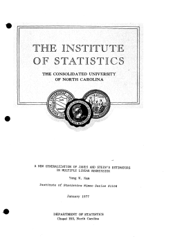
Mortality among Swedish insured
(cf. Swedish Research Board for Actuarial Science (Samuelsson (2008))
Alfa, kvinnor
Alfa, män
−1
−1
−2
−2
−3
−3
−4
−4
−5
−5
−6
−6
−7
−7
−8
−8
−9
30
40
50
60
Ålder
70
80
90
−9
30
40
50
60
Ålder
70
80
90
Figure: The αx parameter for ages 30-90 years (females and males).
Boualem Djehiche KTH Royal Institute of Technology, Stockholm
Statistical estimation techniques in life and non-life insurance An overview
Beta, kvinnor
0.04
Beta, män
0.04
Orginal
Utjämnad
Orginal
Utjämnad
0.035
0.035
0.03
0.03
0.025
0.025
0.02
0.02
0.015
0.015
0.01
0.01
0.005
0.005
0
30
40
50
60
Ålder
70
80
90
0
30
40
50
60
Ålder
70
80
90
Figure: Estimated and smoothed βx parameter for ages 30-90 years (females and
males).
Boualem Djehiche KTH Royal Institute of Technology, Stockholm
Statistical estimation techniques in life and non-life insurance An overview
Kappa, kvinnor
15
10
10
5
5
0
0
−5
−5
−10
−10
−15
−15
−20
1985
1990
1995
Year
Kappa, män
15
2000
2005
−20
1985
1990
1995
År
2000
2005
Figure: Estimated and linearized κ(t) parameter for data 1985-2005 (females and
males).
Boualem Djehiche KTH Royal Institute of Technology, Stockholm
Statistical estimation techniques in life and non-life insurance An overview
κt, kvinnor
15
Kappa, kvinnor
15
Orginal
Utjämnad
Orginal
Utjämnad
10
10
5
5
0
0
−5
−5
−10
−10
−15
−15
−20
1985
1990
1995
År
2000
2005
−20
1985
1990
1995
År
2000
2005
Figure: Estimated and smoothed κ(t) parameter for data 1985-2005 (females and
males).
Boualem Djehiche KTH Royal Institute of Technology, Stockholm
Statistical estimation techniques in life and non-life insurance An overview
Mortality jumps, due to e.g. new life standards or medical development etc.,
are also important to capture in a mortality model, despite the serious
difficulties to perform reliable estimation.
Cox et al. (2010) suggest two types of mortality jump events to the Lee-Carter
model:
log µ(x, t) := α(x) + β(x)κ(t) − G (x, t) + H(x, t),
where
I G (x, t) captures a permanent longevity jump and takes the form
G (x, t) := K (x, t) + D(x, t),
with
K (x, t) :=
∞
X
yj Aj (x)11{t≥ηj } = Jump reduction component,
j=1
and
D(x, t) :=
∞
X
ζi (t−νi )Fi (x)e −ξi (t−νi ) 11{t≥νi } = Trend reduction component.
j=1
I
K (x, t) captures temporary adverse mortality jumps and takes the form
H(x, t) :=
∞
X
bj Bj (x)e −κi (t−τi ) 11{t≥τj } .
j=0
Boualem Djehiche KTH Royal Institute of Technology, Stockholm
Statistical estimation techniques in life and non-life insurance An overview
An age-period-cohort model: Extending Lee-Carter graduation formula
The Lee-Carter model captures the age-period effect, but does not reflect the
possible cohort effect (calender year-age = t − x). A simple model that would
simultaneously capture the age-period-cohort effect would be
log µ(x, t) := α(x) + κ(t) + γ(t − x).
Renshaw and Haberman (2009) suggested the following extension of the
Lee-Carter model to capture the cohort effect (calender year-age = t − x):
log µ(x, t) := β1 (x) + β2 (x)κ(t) + β3 (x)γ(t − x).
(71)
A generalization of this mortality model for data divided into N components
reads
N
X
log µ(x, t) :=
βj (x)κj (t)γj (t − x).
j=1
In a series of papers the Edinburgh teams including Currie, Richards and
co-authors (2003-2012) and Cairns and co-authors (2006-2012) suggest other
extensions and perform deep statistical analysis that seem tune the
age-period-cohort effect when applied to mortality data from England and
Wales, and USA.
Boualem Djehiche KTH Royal Institute of Technology, Stockholm
Statistical estimation techniques in life and non-life insurance An overview
An infinite dimensional approach to mortality modeling
The mortality rate can be viewed as an (infinite dimensional) curve of (x, t).
To capture the high level of uncertainty in projections of future mortality one is
tempted to translate the ”machinery” developed for ”forward” interest rate
yields such as ”the HJM-model under the Musiela parametrization etc..” to
mortality rates. One is tempted to translated the calibration techniques of
interest rate yield curves, to perform hopefully more accurate projections of
future mortality (though with limited data points).
See e.g. Biffis (2005), Biffis and Millossovitch (2006), Biffis and Denuit (2006),
Biffis, Denuit and Devolder (2010), and Tappe and Weber (2013) for further
details.
Boualem Djehiche KTH Royal Institute of Technology, Stockholm
Statistical estimation techniques in life and non-life insurance An overview
References- Incomplete list
Aalen, Odd O.; Hoem, Jan M (1978): Random time changes for multivariate
counting processes. Scand. Actuar. J. no. 2, 81101.
Andersen, P.K:, Borgan, Ø., Gill, R.D., Keiding, N. (1993): Statistical models
based on counting processes, Springer-Verlag, New York, Berlin, Heidelberg.
Brouhns, N., Denuit, D., Vermunt, J. K. (2002): A Poisson log-bilinear
regression approach to the construction of projected lifetables. Insurance:
Mathematics and Economics, 31(3), pp. 373-393.
Barberin, J. ()2008): Heath-Jarrow-Morton modelling of longevity bonds and the
risk minimization of life insurance portfolios. Insur. Math. Econom. 43 (1), pp.
41-55.
Bauer, D. (2008): Stochastic mortality modeling and securitization of mortality
risk. IFA-Schriftenreihe, Ulm.
Bauer, D., Benth, F.E, and Kiesel, R. (2010): Modeling the forward surface of
mortality (Preprint, Univ. Ulm).
Biffis, E. (2005): Affine processes for dynamic mortality and actuarial valuation.
Insur. Math. Econom. 37(3), pp. 443-468.
Boualem Djehiche KTH Royal Institute of Technology, Stockholm
Statistical estimation techniques in life and non-life insurance An overview
References II
Biffis, E. and Denuit, M. (2006): Lee-Carter goes risk-neutral: An application to
the Italian Annuity Market. Giornale dell’Istituto Italiano degli Attuari, Vo. LXIX,
pp.33-53.
Biffis, E., Denuit, M. and Devolder, p. (2010): Stochastic mortality under
measure changes. Scand. Actua. J. (4), pp. 284-311.
Biffis, E.and Millosovitch, P. (2006): A bidimensional approach to mortality risk.
Decision in Economics and Finance, 29(2), pp. 71-94.
Cairns, A.J.G., Blake, D., Dowd, K., Coughlan, G., Epstein, D., Ong, A.,
Balevich, I., (2009): A quantitative comparison of stochastic mortality models
using data from England and Wales and the United States. North American
Actuarial Journal 13(1), pp. 1-35.
Cox, S.H, Lin, Y. and Pedersen, H. (2010): Mortality risk modeling: Applications
to insurance securitization. Insurance: Mathematics and Economics 46(1), pp.
242-253.
Christiansen, M. C., Denuit, M. M. and Lazar, D. (2012): The Solvency II
square-root formula for systematic biometric risk. Insurance: Mathematics and
Economics, 50 (2), pp. 257-265.
Boualem Djehiche KTH Royal Institute of Technology, Stockholm
Statistical estimation techniques in life and non-life insurance An overview
References III
Currie, I. D. (2013): Smoothing constrained generalized linear models with an
application to the Lee-Carter model Statistical Modelling, 13, 69-93.
http://doi:10.1177/1471082X12471373
Currie, I. D. (2012): Forecasting with the age-period-cohort model? (pdf)
Proceedings of 27th International Workshop on Statistical Modelling, Prague,
pp. 87-92.
Currie, I. D. (2012): Forecasting with the age-period-cohort model? (pdf)
Proceedings of 27th International Workshop on Statistical Modelling, Prague,
pp. 87-92.
Currie, I. D. (2011): Modelling and forecasting the mortality of the very old.
(pdf) ASTIN Bulletin, 41, pp. 419-427.
Currie, I. D., M Durban, M., and Eilers, P H C (2004): Smoothing and
forecasting mortality rates Statistical Modelling, 4, 279-298.
Dowd, K., Cairns, A.J.G., Blake, D., Coughlan, G.D., Epstein, D., Khalaf-Allah,
M. (2010): Evaluating the goodness of fit of stochastic mortality models.
Insurance: Mathematics and Economics 47, PP. 255-265.
Fahrenwaldt, M. A. (2013): Sensitivity of life insurance reserves via Markov
semigroups (preprint).
Boualem Djehiche KTH Royal Institute of Technology, Stockholm
Statistical estimation techniques in life and non-life insurance An overview
References IV
Haberman, S. and Renshaw, A. (2009): On age-period-cohort parametric
mortality rate projections. Insurance Math. Econom. 45, no. 2, 255270.
Haberman, S. and Renshaw, A. (2012): Parametric mortality improvement rate
modelling and projecting. Insurance Math. Econom. 50, no. 3, 309333.
Hainaut, D. (2012): Multidimensional LeeCarter model with switching mortality
processes. Insurance: Mathematics and Economics 50 (2), pp. 236-246
Hoem, Jan M. (1969): Markov chain models in life insurance. Blätter Deutsch.
Gesellschaft Vers. math., Vol. 9 (No. 2), pp. 91-107.
Hoem, Jan M. (1969):Purged and partial Markov chains. Scand. Actuar.J., 52,
pp. 147-155.
Hoem, Jan M. (1972): On the statistical theory of analytic graduation Sixth
Berkeley symposium, Proceedings of the Sixth Berkeley Symposium on
Mathematical Statistics and Probability (Univ. California, Berkeley, Calif.,
1970/1971), Vol. I: Theory of statistics, pp. 569600. Univ. California Press,
Berkeley, Calif.
Hoem, Jan M. and Aalen, O.O. (1978): Actuarial values of payment streams.
Scand. Actuar. J. pp. 38-47.
Boualem Djehiche KTH Royal Institute of Technology, Stockholm
Statistical estimation techniques in life and non-life insurance An overview
References V
Hoem, Jan M.(1984): A contribution to the statistical theory of linear
graduation. Insurance Math. Econom. 3, no. 1, 117.
Hyndman, Rob J. and Shahid Ullah, Md. (2007): Robust forecasting of mortality
and fertility rates: A functional data approach. Comput. Stat. Data Analys. 51,
pp. 4942-4956.
Karr, Alan F. (1986): Point processes and their statistical inference. Marcel
Dekker, Inc. New York and Basel.
Lee, R.D. and Carter, L. (1992): Modelling and forecasting the time series of US
mortality. Journal of the American Statistical Association 87, pp. 659-671.
Norberg, R. (1991): Reserves in life and pension insurance. Scand. Actuar. J.
1991, no. 1, 324.
Norberg, R. (1993): Identities for present values of life insurance. Scand. Actuar.
J. pp. 100-106.
Norberg, R. (1999): A theory of bonus prognoses in life insurance. Finance
Stoch. 3, no. 4, 373390.
Boualem Djehiche KTH Royal Institute of Technology, Stockholm
Statistical estimation techniques in life and non-life insurance An overview
References VI
Norberg, R. (2001): On bonus and bonus prognoses in life insurance. Scand.
Actuar. J. 2001, no. 2, 126147.
Norberg, R. (2002): Basic life insurance mathematics. Lecture Notes, University
of Copenhagen.
Norberg, R. (2010): Forward mortality and other vital rates are they the way
forward? Insurance Math. Econom. 47, no. 2, 105112.
Richards, S. J. Kirkby, J. G. and Currie, I. D. (2006): The importance of
year-of-birth in two-dimensional mortality data. British Actuarial Journal, 12 (I),
pp. 5-61.
Richards, S. J. and Currie, I. D. (2009): Longevity risk and annuity pricing with
the Lee-Carter model. British Actuarial Journal, 15, pp. 317-365.
Richards, S. J. (2008): Detecting year-of-birth mortality patterns with limited
data. J. of the Royal Statistical Society, Series A, 171(1), pp. 279-298.
Boualem Djehiche KTH Royal Institute of Technology, Stockholm
Statistical estimation techniques in life and non-life insurance An overview
References VII
Richards, S. J. (2010) Correspondence: Detecting year-of-birth mortality patterns
with limited data. J. of the Royal Statistical Society, Series A, 173(4), pp.
920-924.
Richards, S. J. (2012): A handbook of parametric survival models for actuarial
use. Scand. Actua. J. 4, pp. 233-257.
Samuelsson, E. (2008): Mortality among Swedish insured. Scan. Actua. J.
Volume 2008, Issue 2-3, pp. 184-199.
Steffensen, M. (2006): Surplus-liked life insurance. Scandinavian Actuarial
Journal 1, pp. 1-22.
Tappe, S. and Weber, S. (2013): Stochastic mortality models: An
infinite-dimensional approach (preprint).
Wolthuis, H; Hoem, Jan M (1990): The retrospective premium reserve.
Insurance Math. Econom. 9 (1990), no. 2-3, 229234.
Boualem Djehiche KTH Royal Institute of Technology, Stockholm
Statistical estimation techniques in life and non-life insurance An overview
A systematic graduation technique applicable to mortality and other series
Boualem Djehiche KTH Royal Institute of Technology, Stockholm
Statistical estimation techniques in life and non-life insurance An overview
Trend of a time series as an inverse problem
By graduation we mean extraction of a smooth trend from a time series of data.
A smooth trend ŷ = (ŷ1 , . . . , ŷT ) of a given a time series x = (x1 , . . . , xT ) is a
minimizer of the following problem (Spoerl (1943), Leser (1961), Hodrick and
Prescott (1980, 1997))
T
−2
T
X
X
ŷ (α, x) = arg min
(xt − yt )2 + α
(yt+2 − 2yt+1 + yt )2
y
t=1
!
t=1
for a given α > 0, called the smoothing parameter.
Boualem Djehiche KTH Royal Institute of Technology, Stockholm
Statistical estimation techniques in life and non-life insurance An overview
where,
ŷ (α, x) = arg min kx − y k2 + αkPy k2
y
Py (t) := (yt+2 − yt+1 ) − (yt+1 − yt ),
P is the ((T − 2) × T -matrix)

1
 0

P := 
0
t = 1, 2, . . . , T − 2,
shift operator
−2
1
···
···
1
−2
···
···
···
1
···
1
···
···
···
−2

0
0 
.

1
The unique solution ŷ (α, x) to the optimal problem is
ŷ (α, x) = (IT + αP 0 P)−1 x,
Boualem Djehiche KTH Royal Institute of Technology, Stockholm
(72)
Statistical estimation techniques in life and non-life insurance An overview
A Gaussian random walk model of the trend
To determine the value of the smoothing parameter α, Hodrick and Prescott
suggest the time series x follows a linear mixed model:
x = y + u,
Py = v ,
where (the prior),
u
v
∼ N (0, Σuv ),
with covariance matrix
Σuv :=
σu2 IT
0
Boualem Djehiche KTH Royal Institute of Technology, Stockholm
0
σv2 IT −2
,
Statistical estimation techniques in life and non-life insurance An overview
Since P is of rank T − 2, the signal
v := Py
does not determine a unique y but rather the set of solutions
y := {P 0 (PP 0 )−1 v + Z γ; γ ∈ R 2 }
where the T × 2-matrix Z satisfies
−1
PZ = 0, P 0 PP 0
P + ZZ 0 = IT ,
Z 0 Z = I2 .
(Orthogonal Parametrization)
Boualem Djehiche KTH Royal Institute of Technology, Stockholm
Statistical estimation techniques in life and non-life insurance An overview
(x, y ) is normally distributed:
x
Z
∼N
γ, Σxy ,
y
Z
with covariance matrix
Σxy :=
σu2 IT + σv2 Q
σv2 Q
σv2 Q
σv2 Q
,
where,
Q := P 0 (PP 0 )−1 (PP 0 )−1 P,
Boualem Djehiche KTH Royal Institute of Technology, Stockholm
QZ = 0,
Z 0 Q = 0,
Statistical estimation techniques in life and non-life insurance An overview
and
Q[
σu2
σ2
I + Q]−1 = [ u2 IT + Q]−1 Q,
2 T
σv
σv
which yields that
Q[
σu2
IT + Q]−1 Z = 0.
σv2
The maximum likelihood estimator of γ is
argminγ (x − Z γ)0 [σu2 IT + σv2 Q]−1 (x − Z γ) = Z 0 x.
Boualem Djehiche KTH Royal Institute of Technology, Stockholm
Statistical estimation techniques in life and non-life insurance An overview
Noise-to-Signal Ratio
Theorem 1 (Hodrick and Prescott (1997))
α = σu2 /σv2 .
Hodrick and Prescott derived this equality using
ŷ (α, x) ≈ E [y |x],
from signal-extraction techniques which is widely used in Signal Processing.
First to prove Theorem 1 is (Schlicht (2005):
Theorem 2 (Schlicht (2005))
α = σu2 /σv2 and γ = Z 0 x (ML-estimator of γ)
if and only if
ŷ (α, x) = E [y |x].
0
(Recall ŷ (α, x) := (IT + αP P)−1 x)
Boualem Djehiche KTH Royal Institute of Technology, Stockholm
Statistical estimation techniques in life and non-life insurance An overview
Proposition (Dermoune-D-Rahmania(2009))
α∗ = σu2 /σv2 = arg min kE [ y | x] − y (α, x)k2 .
α>0
Moreover, the error (optimal gap)
E [ y | x] − y (α∗ , x) = Z γ − Z 0 x
is a centered Gaussian vector with covariance matrix
cov Z Z 0 x − γ = σu2 ZZ 0 .
In particular,
E [kE [ y | x] − y (α∗ , x)k2 ]
= E [kZ (γ − Z 0 x) k2 ]
= σu2 trace(ZZ 0 ) = 2σu2 .
Boualem Djehiche KTH Royal Institute of Technology, Stockholm
Statistical estimation techniques in life and non-life insurance An overview
For US real GNP time series, the smoothing parameter α is determined in two
ways:
I
Hodrick and Prescott (1980, 1997) finds α∗ = 1600 using a prior view
based on macroeconomics arguments: σu = 5% and σv = 1/8% in the
rate of the growth in a quarter.
I
Schlicht (2005) finds α∗ = 2.40, using a complicated ML-estimator which
is a fixed point of a highly nonlinear matrix equation. The consistency of
the ML-estimator is still open.
Boualem Djehiche KTH Royal Institute of Technology, Stockholm
Statistical estimation techniques in life and non-life insurance An overview
A consistent estimator of the noise-to-signal ratio α
We use observations from the centered Gaussian and stationary (thanks to P)
time series Px:
Px = v + Pu ∼ N (0, σv2 IT −2 + σu2 PP 0 ).
The elements of the covariance matrix are
σv2 δij + σu2 (PP 0 )ij = r|i−j| ,
where,
 2
σv + 6σu2 ,



−4σu2 ,
rk =
σ2 ,


 u
0,
Boualem Djehiche KTH Royal Institute of Technology, Stockholm
if k = 0;
if k = 1;
if k = 2;
otherwise.
Statistical estimation techniques in life and non-life insurance An overview
A classical fact that (see e.g. Chapter 7 in Brockwell and Davis (1991))
r̂k =
TX
−2−k
1
Px(j)Px(j + k),
(T − 2) − k j=1
k = 0, 1, 2,
is an unbiased estimator of rk = E [Px(s)Px(s + k)] in the sense that E [r̂k ] = rk .
Theorem
The following statistics
1
α
b=−
4
!−1
P −2
(T − 3) Tj=1
Px(j)2
3
+
P −3
2
(T − 2) Tj=1
Px(j)Px(j + 1)
(73)
based on the time series of observation Px, is a consistent estimator of the
smoothing parameter α.
Boualem Djehiche KTH Royal Institute of Technology, Stockholm
Statistical estimation techniques in life and non-life insurance An overview
Performance of different estimates of the statistics α̂
• α = 0.5 based on 5000 simulations.
T-2
1000
2500
5000
mean(α̂)
0.512
0.503
0.501
standard deviation(α̂)
0.09
0.06
0.04
• α = 10 based on 5000 simulations.
T-2
1000
7000
14000
percentage of (α̂ < 0)
0.255
0.044
0.010
standard deviation(α̂)
548
226
65
Boualem Djehiche KTH Royal Institute of Technology, Stockholm
Statistical estimation techniques in life and non-life insurance An overview
Estimating α for US real GNP time series under the period
01-01-1947–01-01-2006
For US real GNP time series, the smoothing parameter α is estimated as
follows.
• Using Eq. (1), α∗ = 0.41.
• Hodrick and Prescott (1980, 1997) find α∗ = 1600.
• Schlicht (2005) finds α∗ = 2.40.
Boualem Djehiche KTH Royal Institute of Technology, Stockholm
Statistical estimation techniques in life and non-life insurance An overview
US Real GNP
Estimated trend
Trend using Schlicht estimator
Hodrick−Prescott trend
4200
4000
3800
3600
3400
3200
3000
2800
2600
65
70
75
Boualem Djehiche KTH Royal Institute of Technology, Stockholm
80
85
90
95
100
Statistical estimation techniques in life and non-life insurance An overview
1
0.5
0
−0.5
Autocorrelation function of the noise component using alpha=1600.
Boualem Djehiche KTH Royal Institute of Technology, Stockholm
Statistical estimation techniques in life and non-life insurance An overview
1
0.8
0.6
0.4
0.2
0
−0.2
−0.4
Autocorrelation function of the noise component using alpha=2.4028.
Boualem Djehiche KTH Royal Institute of Technology, Stockholm
Statistical estimation techniques in life and non-life insurance An overview
1
0.5
0
−0.5
Autocorrelation function of the noise component using alpha=0.4137.
Boualem Djehiche KTH Royal Institute of Technology, Stockholm
Statistical estimation techniques in life and non-life insurance An overview
Calibration
Estimated values of the smoothing parameter α. The values of α̂ are based on
the estimator given by Eq. (1) and α∗ are obtained using the Schlicht’s
estimator.
x
US real GNP
GBP
Euro
CHF
JPY
α̂
0.4137
0.3734
0.3675
0.5896
0.4489
α∗
2.4028
1.2998
0.67173
1.4592
1.8383
x
S&P 500
Nasdaq
Dow Jones
FTSI
Nikkei
α̂
0.4963
0.5152
0.6417
0.4125
0.4721
α∗
8.1615
3.2756
1.1907
3.0841
2.4028
Boualem Djehiche KTH Royal Institute of Technology, Stockholm
Statistical estimation techniques in life and non-life insurance An overview
The Hodrick-Prescott Multivariate filter
The Hordrick-Prescott Multivariate filter (HPMV) seeks to estimate the
unobserved variable y as a solution to the following minimization problem
arg min(||x − y ||2 + α1 ||Py ||2 + α2 ||z − βy ||2 ),
y
given the following dynamics:

 x = y + u,
z := x ∗ − dX = βy + ξ,

Py = v ,
(74)
(75)
where, xt∗ is another explanatory variable (the Phillips curve) that can be
explained by the unobserved variable y , and X is an exogenous variable affected
by the parameter d. with


u
 ξ  ∼ N (0, Σ),
(76)
v
Boualem Djehiche KTH Royal Institute of Technology, Stockholm
Statistical estimation techniques in life and non-life insurance An overview
σu2 IT
Σ :=  0
0

0
σξ2 IT
0

0
.
0
σv2 IT −2
the time series (x, z) can be represented in terms of (u, v , ξ) as
x = u + P 0 (PP 0 )−1 v + Z γ,
z = ξ + βP 0 (PP 0 )−1 v + βZ γ,
(77)
for some γ ∈ R2 .
In view of (77),

Σxyz




x
Z
 z  ∼ N  βZ  γ, Σxzy  ,
y
Z
 2
σu IT + σv2 Q
βσv2 Q
σv2 Q
2
2
2
2

βσ
Q
σ
I
+
βσ
Q
βσ
v
v
vQ
ξ T
=

σv2 Q
βσv2 Q
σv2 Q
(78)


,

where,
Q := P 0 (PP 0 )−1 (PP 0 )−1 P
Boualem Djehiche KTH Royal Institute of Technology, Stockholm
Statistical estimation techniques in life and non-life insurance An overview
The unique solution ŷ to Problem (74) is
ŷ = a(IT + bP 0 P)−1 w ,
where, a := 1/(1 + α2 β 2 ), b := α1 /(1 + α2 β 2 ) and w := x + α2 βz.
Proposition The best smoothing parameters of the HPMV filter according to
Schilcht Criterion are those positive parameters α1∗ and α2∗ for which
α1∗ /α1e = 1 + α2∗ β 2 (α2∗ /α2e − α1∗ /α1e ) ,
where,
α1e
=
σu2 /σv2
and
α2e
=
(79)
σu2 /σξ2 .
In particular,
(1) α1∗ = α1e if and only if α2∗ = α2e .
(2) If α1∗ /α1e < 1, then necessarily α2∗ /α2e < α1∗ /α1e .
(3) If α1∗ /α1e > 1, then necessarily α2∗ /α2e > α1∗ /α1e .
Boualem Djehiche KTH Royal Institute of Technology, Stockholm
Statistical estimation techniques in life and non-life insurance An overview
The following statistics
α
b1e
1
=−
4
!−1
P −2
(T − 3) Tj=1
Px(j)2
3
+
,
P −3
2
(T − 2) Tj=1
Px(j)Px(j + 1)
PT −3
j=1
Px(j)Px(j + 1)
j=1
Pz(j)Pz(j + 1)
α
b2e = PT −3
,
and
βb2 =
2(T − 3)
PT −2
2(T − 3)
PT −2
j=1
j=1
Pz(j)2 + 3(T − 2)
PT −3
Pz(j)Pz(j + 1)
+ 3(T − 2)
PT −3
Px(j)Px(j + 1)
Px(j)2
j=1
j=1
,
based on the time series of observations Px and Pz, are consistent estimators
of the smoothing parameters α1e , α2e and the parameter β.
Boualem Djehiche KTH Royal Institute of Technology, Stockholm
Statistical estimation techniques in life and non-life insurance An overview
Calibration
T-2
500
1000
5000
(mean(α̂e1 ), std(α̂e1 ))
(1.13, 0.61)
(1.05, 0.33)
(1.00,0.11)
(mean(α̂e2 ), std(α̂e2 ))
(1.01, 0.16)
(1.00, 0.11)
(1.00, 0.05)
(mean(β̂), std(β̂))
(0.47, 0.29)
(0.47, 0.22)
(0.49, 0.08)
Table: Performance of different estimates of the statistics on αe1 = 1, αe2 = 1 and
β = 0.5 based on 1000 simulations.
Boualem Djehiche KTH Royal Institute of Technology, Stockholm
Statistical estimation techniques in life and non-life insurance An overview
T-2
500
1000
5000
(mean(α̂e1 ), std(α̂e1 ))
(1.13, 0.61)
(1.05, 0.33)
(1.00,0.11)
(mean(α̂e2 ), std(α̂e2 ))
(0.50, 0.09)
(0.50, 0.06)
(0.50, 0.02)
(mean(β̂), std(β̂))
(2.06, 0.43)
(2.01, 0.23)
(2.00, 0.10)
Table: Performance of different estimates of the statistics on αe1 = 1, αe2 = 0.5 and
β = 2 based on 1000 simulations.
T-2
500
1000
5000
(mean(α̂e1 ), std(α̂e1 ))
(1.13, 0.61)
(1.05, 0.33)
(1.00,0.11)
(mean(α̂e2 ), std(α̂e2 ))
(16.30, 2.73)
(16.14, 1.84)
(15.96, 0.84)
(mean(β̂), std(β̂))
(0.19, 0.05)
(0.20, 0.03)
(0.19, 0.01)
Table: Performance of different estimates of the statistics on αe1 = 1, αe2 = 16 and
β = 0.2 based on 1000 simulations.
Boualem Djehiche KTH Royal Institute of Technology, Stockholm
Statistical estimation techniques in life and non-life insurance An overview
Boualem Djehiche KTH Royal Institute of Technology, Stockholm
Statistical estimation techniques in life and non-life insurance An overview
Multivariate HP filter
Example Consider the following two-dimensional HP-filter:
x i = y i + u i , Py i = v i , i = 1, 2,
where, the noises u 1 and u 2 , respectively v 1 and v 2 , may be correlated.
P 0
A :=
,
0 P
we get the following two-dimensional HP-filter:
x = y + u, Ay = v .
Boualem Djehiche KTH Royal Institute of Technology, Stockholm
Statistical estimation techniques in life and non-life insurance An overview
u
v
with covariance matrix
∼ N (0, Σuv ).
Σuv :=
Σu
0
0
Σv
.
(x, y ) is normally distributed:
x
Z
∼N
γ, Σxy ,
y
Z
with covariance matrix
Σxy :=
Σu + Qv
Qv
Qv
Qv
,
where,
Qv := A0 (AA0 )−1 Σv (AA0 )−1 A
E [ y | x] = Z γ + Qv [Σu + Qv ]−1 (x − Z γ).
Boualem Djehiche KTH Royal Institute of Technology, Stockholm
Statistical estimation techniques in life and non-life insurance An overview
The maximum likelihood estimator of γ is
γ̂ = argminγ (x − Z γ)0 [Σu + Qv ]−1 (x − Z γ)
= Z 0 Σu ZZ 0 [Σu + Qv ]−1 x.
We suggest the following multivariate HP-filter.
Definition A multivariate HP-trend minimizes the following weighted sum
ŷ (Σ, Ω)) = argminy (x − y )0 Σ−1 (x − y ) + y 0 A0 Ω−1 Ay ,
where (Σ, Ω) is a pair of positive definite matrices with appropriate dimensions
that acts as a smoothing parameter.
Boualem Djehiche KTH Royal Institute of Technology, Stockholm
Statistical estimation techniques in life and non-life insurance An overview
Multivariate noise-to-signal ’ratio’
We suggest to find the best smoothing parameter (Σ∗ , Ω∗ ) for which
(Σ∗ , Ω∗ ) = argmin{(Σ,Ω)∈A} kE [ y | x] − y ((Σ, Ω), x) k2 .
(80)
in the following class A of admissible matrices.
A
= {(Σ, Ω) posi. def. s.t. ŷ − Z γ̂ is orthogonal to Z γ̂}
= {(Σ, Ω) posi. def. s.t. ΣΠ = ΠΣ}.
where,
Π = A0 (AA0 )−1 A.
Boualem Djehiche KTH Royal Institute of Technology, Stockholm
Statistical estimation techniques in life and non-life insurance An overview
Proposition The pairs of invertible matrices (Σ∗ , Ω∗ ) ∈ A are optimal i.e.
(Σ∗ , Ω∗ ) = argmin{(Σ,Ω)∈A} kE [ y | x] − y ((Σ, Ω), x) k2 .
if and only if they are solutions of the following equation.
−1
Σ∗ A0 Ω∗−1 Σv (AA0 )−1 A = Σu − Z Z 0 [Σu + Qv ]−1 Z
Z 0.
(81)
(82)
In particular, given Σ∗ ,
Ω∗−1 =
0 −1
(AA )
∗−1
AΣ
0
Σu − Z Z [Σu + Qv ]
Boualem Djehiche KTH Royal Institute of Technology, Stockholm
−1
Z
−1
Z
0
A0 Σ−1
v .
Statistical estimation techniques in life and non-life insurance An overview
Moreover, the error (optimal gap)
E [ y | x]−y ((Σ∗ , Ω∗ ), x) =
−1
Z γ − Z 0 [Σu + Qv ]−1 Z
Z 0 [Σu + Qv ]−1 x
is a centered Gaussian vector with covariance matrix
=
cov Z Σu ZZ 0 [Σu + Qv ]−1 x − γ
−1
Z Z 0 [Σu + Qv ]−1 Z
Z 0.
Boualem Djehiche KTH Royal Institute of Technology, Stockholm
Statistical estimation techniques in life and non-life insurance An overview
Solvability of Eq. (82)
Lemma Eq. (82) is solvable if and only if
ΠΣu (IdT − Π) = 0,
(if and only if
ΠΣu = Σu Π.)
(83)
where,
Π = A0 (AA0 )−1 A
In this case, (82) reduces to
ΣA0 Ω−1 Σv (AA0 )−1 A = Σu Π.
Boualem Djehiche KTH Royal Institute of Technology, Stockholm
(84)
Statistical estimation techniques in life and non-life insurance An overview
Theorem Assume ΠΣu = Σu Π. Then (Σ, Ω) ∈ A is optimal if and only if
(Σ, Ω) satisfies
0
0 −1
Σ−1
u ΣA = A Σv Ω.
In particular,
y ((Σ, Ω) , x) = y ((Σu , Σv ) , x) ,
for all x ∈ R
dT
.
Moreover, the covariance matrix of the error (optimal gap) is
cov (E [ y | x] − y ((Σ, Ω), x)) = ZZ 0 Σu ZZ 0 .
Boualem Djehiche KTH Royal Institute of Technology, Stockholm
Statistical estimation techniques in life and non-life insurance An overview
A final remark
(a) Using, ΠA0 = A0 also yields that
−1
ŷ = IdT + ΠΣu ΠA0 Σ−1
x,
v A
We only need the variance of Πu which is ΠΣu Π and Σv , thus similar to α
in the standard HP-filter.
(b) (Σu , Σv ) is optimal i.e. it satisfies (82).
In particular, if Ω = Σv = σv2 Id(T −k) , we have
ŷ =
IdT
Σu
+ 2 A0 A
σv
−1
x,
suggesting an optimal smoothing parameter α = Σu /σv2 which is a matrix.
Boualem Djehiche KTH Royal Institute of Technology, Stockholm
Statistical estimation techniques in life and non-life insurance An overview
(c) The pair of matrices (Σ∗ , Σv ) is optimal, for any invertible matrix Σ∗ that
satisfies
Σ∗ Π = ΣΠ = ΠΣ,
is equivalent to choosing Σ∗ of the form
var (Πu)
Σ∗ =
0
0
L
.
(85)
written in the basis
q
√
A0 g1 / λ1 , . . . , A0 gd(T −k) / λd(T −k) , Z1 , . . . , Zkd ,
where λi are the eigenvalues of AA0 and g1 , . . . , gd(T −k) an orthonormal
set of eigenvectors corresponding to λi , i = 1, . . . , λd(T −k) . The matrix L
is any arbitrary dk × dk-matrix. When L = var ((I − Π)u), Σ∗ = Σu .
Boualem Djehiche KTH Royal Institute of Technology, Stockholm
Statistical estimation techniques in life and non-life insurance An overview
Optimal Spline Smoothing of the Hodrick-Prescott Trend
The HP-filter is of limited use for any analysis of the behavior of x in any of
the time intervals (tj−1 , tj ) unless an appropriate smooth curve fit, such as
polynomial splines, between the tj ’s is used.
Boualem Djehiche KTH Royal Institute of Technology, Stockholm
Statistical estimation techniques in life and non-life insurance An overview
Spline smoothing of the HP-trend
We suggest a smooth curve fit which is consistent with the HP-filter: The
chosen smooth curve y (t) is such that
y (tj ) = ȳj ,
j = 1, . . . , n.
That is, the chosen smooth curve y (t) should minimize the following cost
functional
Z tn
2
J(y ) = kx − ȳ k2 + λ
y (2) (t) dt + ȳ T P T WP ȳ ,
t1
for some smoothing parameters (λ, W ), with λ > 0 and W positive definite
matrix.
Moreover, the smoothing parameters should be optimal:
(λ∗ , W ∗ ) = arg min{λ>0,W positive definite} kE[ȳ | x] − ȳ (λ, W , x)k2 .
Boualem Djehiche KTH Royal Institute of Technology, Stockholm
Statistical estimation techniques in life and non-life insurance An overview
A smoothing cubic B-spline trend
We suggest to look for a smoothing cubic spline curve y (t) which minimizes J
of the form

x = ȳ + u,



P ȳ = v ,
y (t) = b(t)T τ,



ȳ = B T τ,
where,
• b(t) is an (n × m) cubic smoothing B-spline,
• B = (b(t1 ), . . . , b(tn )) ∈ Rn×m ,
• τ = (τ1 , . . . , τm )T ∈ Rm is the new control parameter,
• ȳi := y (ti ), i = 1, . . . , n.
Boualem Djehiche KTH Royal Institute of Technology, Stockholm
Statistical estimation techniques in life and non-life insurance An overview
With y (t) = b(t)T τ,
Z
tn
(y (2) (t))2 dt = τ T G τ,
t1
where, G ∈ Rm×m is the Gramian associated to b:
Z tn 2
d b(t) d 2 b T (t)
dt.
G =
dt 2
dt 2
t1
The cost functional J(y ) becomes
J(τ ) = kx − ȳ k2 + λ
tn
Z
2
y (2) (t) dt + ȳ T P T WP ȳ
t1
= x T x − 2τ T B T x + τ T Lτ,
L := λG + B T (In + P T WP)B
is positive definite (see Kono et al. (2005)).
Boualem Djehiche KTH Royal Institute of Technology, Stockholm
Statistical estimation techniques in life and non-life insurance An overview
The unique minimizer of J is
τ̂ = L−1 B T x,
which, in terms of (λ, W ) and x, reads
τ̂ (λ, W , x) = (λG + B T (In + P T WP)B)−1 B T x.
Hence, our cubic B-spline optimal trend is
ŷ (t) = b(t)T (λG + B T (In + P T WP)B)−1 B T x,
Boualem Djehiche KTH Royal Institute of Technology, Stockholm
t ∈ [t1 , tn ].
Statistical estimation techniques in life and non-life insurance An overview
Using
E[ ȳ | x] = ȳ (
σu2
, x) =
σv2
In +
σu2 T
P P
σv2
−1
x.
(λ∗ , W ∗ ) = arg min{λ>0,W positive definite} kE[ȳ | x] − ȳ (λ, W , x)k2 .
if and only if (λ∗ , W ∗ ) satisfy the following balance equation
∗
T
T
∗
−1
B(λ G + B (In + P W P)B)
T
B x=
σ2
In + u2 P T P
σv
!−1
x.
or
W∗ =
σu2
In−2 − λ∗ (PP T )−1 P(BB T )−1 BGB T (BB T )−1 P T (PP T )−1 .
σv2
Theorem (D., Marcus and Rahmania (2011))
• The balance equation has always has a feasible solution.
• The cubic B-spline optimal trend is
ŷ (t) = b(t)T B T (BB T )−1 (In +
Boualem Djehiche KTH Royal Institute of Technology, Stockholm
σu2 T −1
P P) x.
σv2
Statistical estimation techniques in life and non-life insurance An overview
A numerical example
We use three different estimators of the noise-to-signal ratio σu2 /σv2 :
2
2
• αDDR = σ\
u /σv proposed in Dermoune et al. (2008),
2
2
σ\
u /σv
n
1
= max 0, −
4
!−1
P
2
o
(n − 3) n−2
3
j=1 ξj
,
+
Pn−3
2
(n − 2) j=1 ξj ξj+1
(86)
where, ξ = Px.
• The Generalized Cross Validation (GCV) estimator as solved efficiently in
Wienert (2007) and Weinert (2009).
• The one proposed by Hodrick and Prescott (1997), αHP = 1600, for
quarterly time series.
Boualem Djehiche KTH Royal Institute of Technology, Stockholm
Statistical estimation techniques in life and non-life insurance An overview
αDDR
αGCV
αHP
US GNP
0.321
0.240
1600
GBP/USD
0.446
0.198
1600
S&P500
0.267
3.65e-3
1600
Table: estimated values of the noise-to-signal ratio σu2 /σv2 .
Boualem Djehiche KTH Royal Institute of Technology, Stockholm
Statistical estimation techniques in life and non-life insurance An overview
Figure: US quarterly GNP from 1947 Q1 to 2010 Q2. Index number 2005=100.
Boualem Djehiche KTH Royal Institute of Technology, Stockholm
Statistical estimation techniques in life and non-life insurance An overview
Figure: Daily GBP/USD close prices from 03/31/03 to 10/01/10.
Boualem Djehiche KTH Royal Institute of Technology, Stockholm
Statistical estimation techniques in life and non-life insurance An overview
Figure: Monthly close prices of S&P500 from Dec 1987 to Aug 2010.
Boualem Djehiche KTH Royal Institute of Technology, Stockholm
Statistical estimation techniques in life and non-life insurance An overview
Main References I
Dermoune, A., Djehiche, B. and Rahmania, N. (2008): Consistent estimators of
the smoothing parameter in the Hodrick-Prescott Filter. J. Japan Statist. Soc.,
Vol. 38 (No. 2), pp. 225-241.
Dermoune, A., Djehiche, B. and Rahmania, N. (2009): Multivariate extension of
the Hodrick-Prescott Filter- Optimality and characterization. Studies in Nonlinear
Dynamics and Econometrtics., (13), pp. 1-33.
Djehiche, B., Marcus, M., and Rahmania, N. (2011): On a Graduation Problem
involving both the Hodrick-Prescott Filter and Optimal Spline Smoothing. Far
East J. Theoretical Statistics, 36(1), 1-19.
Djehiche, B. and H. Nassar, H. (2012): A Functional Hodrick-Prescott filter
(preprint).
Djehiche, B. and Rahmania, N. (2013): Modeling and estimating correlated
growth and business cycles in a multivariate Hodrick-Prescott filter. Far East J.
Theoretical Statistics, (42)1, 41-70.
Boualem Djehiche KTH Royal Institute of Technology, Stockholm
Statistical estimation techniques in life and non-life insurance An overview
Main References II
Hoem, Jan M. (1972): On the statistical theory of analytic graduation Sixth
Berkeley symposium, Proceedings of the Sixth Berkeley Symposium on
Mathematical Statistics and Probability (Univ. California, Berkeley, Calif.,
1970/1971), Vol. I: Theory of statistics, pp. 569-600. Univ. California Press,
Berkeley, Calif.
Hoem, Jan M.(1984): A contribution to the statistical theory of linear
graduation. Insurance Math. Econom. 3, no. 1, 1-17.
Hodrick, R. and Prescott, E. C. (1997): Postwar U.S. business cycles: An
empirical investigation. Journal of Money, Credit and Banking. 29(1), 1-16.
Kano, H., Nakata, H. and Martin, C. (2005): Optimal curve fitting and
smoothing using normalized uniform B-splines: A tool for studying complex
systems. Appl. Math. and Comput. 169(1), 96-128.
Schlicht, E. (2005): Estimating the smoothing parameter in the so-called
Hodrick-Prescott filter. J. Japan Statist. Soc., Vol. 35 No. 1, 99-119.
Boualem Djehiche KTH Royal Institute of Technology, Stockholm
Statistical estimation techniques in life and non-life insurance An overview
Stochastic claims reserving in disability insurance
Outline
I
Disability inception model
I
Recovery model
I
Stochastic claims reserving
Based on
I
H. Aro, B. Djehiche and B. Löfdahl (2013): Stochastic modelling of
disability insurance in a multi-period framework (to appear in
Scandinavian Actuarial Journal).
Boualem Djehiche KTH Royal Institute of Technology, Stockholm
Statistical estimation techniques in life and non-life insurance An overview
Disability inception
A plot of age vs. year vs. inception frequencies for females is displayed below.
60
60
50
2000
40
2005
30
2010
50
2000
40
2005
30
2010
Inception seems to be strongly time- and age-dependent. How can we model
this behaviour?
Boualem Djehiche KTH Royal Institute of Technology, Stockholm
Statistical estimation techniques in life and non-life insurance An overview
Disability inception
I
Let Ex,t denote the number of healthy individuals with age in [x, x + 1) at
the beginning of time period t
I
Let Dx,t denote the number of individuals among Ex,t with disability
inception in the interval [t, t + 1)
I
Goal: model inception over time, t = 0, 1, 2, . . .
I
Assume Dx,t is binomially distributed given Ex,t :
Dx,t ∼ Bin(Ex,t , px,t )
where px,t is the inception probability of an x-year-old.
Boualem Djehiche KTH Royal Institute of Technology, Stockholm
Statistical estimation techniques in life and non-life insurance An overview
Disability inception
I
In order to reduce the dimensionality of the problem and achieve some
level of smoothness, we employ logistic regression:
px,t := log
n
px,t X i i
=
νt φ (x),
1 − px,t
i=1
where φi (x) are age-dependent basis functions and νti time-varying
stochastic risk factors.
I
Changing notation, pνt (x) = px,t , we invert the expression above,
obtaining
Pn
i i
exp
i=1 νt φ (x)
P
pνt (x) =
1 + exp( ni=1 νti φi (x))
I
This guarantees that the probabilities pνt (x) ∈ (0, 1).
Boualem Djehiche KTH Royal Institute of Technology, Stockholm
Statistical estimation techniques in life and non-life insurance An overview
Disability inception
Given historical values of Dx,t and Ex,t , and a set of basis functions {φi }, the
log-likelihood function for yearly values of νt ∈ Rn can be written
l(νt ) =
Xh
x∈X
Dx,t
n
X
νti φi (x) − Ex,t log 1 + exp
i=1
n
X
i
νti φi (x)
+ ct .
i=1
I
If the basis functions are linearly independent, −l(νt ) is strictly convex.
I
Minimizing using methods from numerical optimization yields unique
estimates of νt .
I
Question: How do we determine the basis functions?
Boualem Djehiche KTH Royal Institute of Technology, Stockholm
Statistical estimation techniques in life and non-life insurance An overview
Disability inception
I
I
The basis functions can be chosen by the user, according to some criteria
Desired properties of pνt (·), e.g. continuity or smoothness w.r.t. x, is
achieved by choosing continuous or smooth φi (·)
I
I
I
Population characteristics can be taken into account
Suitable choices of basis functions gives the risk factors concrete
interpretations
Alternatively, an optimal basis can be extracted from the data using
functional principal component analysis.
I
Yields better model fit, but harder to interpret results.
Boualem Djehiche KTH Royal Institute of Technology, Stockholm
Statistical estimation techniques in life and non-life insurance An overview
Disability inception
I
Consider the model
pνt (x) = νt1 φ1 (x) + νt2 φ2 (x),
where the basis functions are linear on x ∈ [25, 64]:
1
φ (x) =
I
64 − x
39
,
2
φ (x) =
x − 25
39
A linear combination of φ1 and φ2 is then also linear.
Boualem Djehiche KTH Royal Institute of Technology, Stockholm
Statistical estimation techniques in life and non-life insurance An overview
Disability inception
1
1
1
0.9
0.9
0.9
0.8
0.8
0.8
0.7
0.7
0.7
0.6
0.6
0.6
0.5
0.5
0.5
0.4
0.4
0.4
0.3
0.3
0.3
0.2
0.2
0.2
0.1
0.1
0
25
30
35
40
45
50
55
60
0
25
0.1
30
35
40
45
50
55
60
0
25
30
35
40
45
50
55
60
Figure: Left: two basis functions. Centre: basis functions scaled with risk factor values
0.4 and 0.6. Right: the resulting linear combination. Note: φ1 (25) = φ2 (64) = 1, and
φ1 (64) = φ2 (25) = 0.
Boualem Djehiche KTH Royal Institute of Technology, Stockholm
Statistical estimation techniques in life and non-life insurance An overview
Disability inception
I
Under this model, the logistic inception probability of a 25-year old is
given by
pνt (25) = νt1 φ1 (25) + νt2 φ2 (25) = νt1 .
I
Similarly, for a 64-year old we have
pνt (64) = νt2 .
I
An x-year old can be seen as a convex combination of a 25-year old and a
64-year old.
I
Inception for the population described by only νt1 and νt2 .
Boualem Djehiche KTH Royal Institute of Technology, Stockholm
Statistical estimation techniques in life and non-life insurance An overview
Disability inception
60
60
50
2000
40
2005
30
2010
50
2000
40
2005
30
2010
Figure: Left: Inception frequencies per 5-year age groups, females. Right: Model
surface.
Boualem Djehiche KTH Royal Institute of Technology, Stockholm
Statistical estimation techniques in life and non-life insurance An overview
Recovery from disability
I
Recovery from disability is slightly more complicated
I
I
I
The probability of recovering from illness depends on the amount of time
spent in the ’ill’ state.
This is known as a semi-Markov property.
We extend the disability inception model above to the semi-Markov case,
and apply it to recovery modelling.
Boualem Djehiche KTH Royal Institute of Technology, Stockholm
Statistical estimation techniques in life and non-life insurance An overview
Recovery model
I
Let Ex,d,t denote the number of individuals with disability inception age in
[x, x + 1) and disability duration d at some point in the time period
[t, t + 1).
I
Let Rx,d,t denote the number of individuals among Ex,d,t that recover
during [d, d + ∆d) and [t, t + 1).
I
Goal: model recovery over time, t = 0, 1, 2, . . .
I
Assume Rx,d,t is binomially distributed given Ex,d,t :
Rx,d,t ∼ Bin(Ex,d,t , px,d,t )
where px,d,t is the probability that an individual, with disability inception
age in [x, x + 1) and disability duration d at some point in [t, t + 1),
recovers before duration d, d + ∆d.
Boualem Djehiche KTH Royal Institute of Technology, Stockholm
Statistical estimation techniques in life and non-life insurance An overview
Recovery model
I
We propose the following logistic regression model:
pνt (x, d) =
n
X
φi (x)
i=1
k
X
νti,j ψ j (d),
j=1
where φi and ψ j , are age and duration dependent basis functions,
respectively, and νti,j are stochastic risk factors.
I
Compare with inception model:
pνt (x) =
n
X
νti φi (x).
i=1
I
Basically the same model, extended one dimension.
Boualem Djehiche KTH Royal Institute of Technology, Stockholm
Statistical estimation techniques in life and non-life insurance An overview
Recovery model
I
I
Likelihood also has the same structure as before.
Strict convexity if
I
I
I
{φi } lin. indep.
{ψ i } lin. indep.
Again, we estimate νt using numerical optimization.
Boualem Djehiche KTH Royal Institute of Technology, Stockholm
Statistical estimation techniques in life and non-life insurance An overview
Recovery model
I
Consider the model
pνt (x, d) = φ1 (x)
3
X
νt1,j ψ j (d) + φ2 (x)
j=1
3
X
νt2,j ψ j (d)
j=1
where φ and ψ are given by:
64 − x
,
39
x − 25
,
39
1
=
2
=
1
=
1,
2
=
3
=
d,
√
d.
φ (x)
φ (x)
ψ (d)
ψ (d)
ψ (d)
Boualem Djehiche KTH Royal Institute of Technology, Stockholm
Statistical estimation techniques in life and non-life insurance An overview
Recovery model
I
The recovery probabilities for a 25-year old are given by
pνt (25, ·)
=
φ1 (25)
3
X
νt1,j ψ j (·) + φ2 (25)
j=1
=
3
X
3
X
νt2,j ψ j (·)
j=1
νt1,j ψ j (·),
j=1
determined by νt1,1 , νt1,2 , νt1,3 .
I
Similarly, the recovery probabilities for a 64-year old determined by
νt2,1 , νt2,2 , νt2,3 .
I
An x-year old can be seen as a convex combination of a 25-year old and a
64-year old.
Boualem Djehiche KTH Royal Institute of Technology, Stockholm
Statistical estimation techniques in life and non-life insurance An overview
Recovery model
I
Let an x-year old’s illness duration be the r.v. D.
I
The probability that the illness lasts longer than d years is given by
d/∆d−1
λ(x, d) = Pνt (D > d) =
Y
(1 − pνt (x, n∆d)).
n=0
I
These are analogous to survival curves.
Boualem Djehiche KTH Royal Institute of Technology, Stockholm
Statistical estimation techniques in life and non-life insurance An overview
Recovery model
2006
0
0
60
5
60
5
55
55
50
50
45
10
40
45
10
40
35
35
30
15
25
30
15
25
Figure: Left: Conditional recovery probabilities. Right: Recovery surface, females,
calendar year 2006.
Boualem Djehiche KTH Royal Institute of Technology, Stockholm
Statistical estimation techniques in life and non-life insurance An overview
Claims reserving
Let Xt denote the state of an individual at time t, and let i denote the ’ill’
state.
I
Classical approach: estimate νt and use the measure Pνt for computing
premiums and reserves.
I
The initial reserve is given by the expected value of the discounted
monthly payments,
i
hX
V = E
I {Xtk = i}e −rtk X0 = i, ν = ν̂
k
=
X
P(Xtk = i|X0 = i, ν = ν̂)e −rtk .
k
I
Assuming independence, all systematic risk vanishes.
I
Let portfolio grow to infinity and be happy (LLN).
Boualem Djehiche KTH Royal Institute of Technology, Stockholm
Statistical estimation techniques in life and non-life insurance An overview
Stochastic claims reserving
I
New approach: model future probabilities of inception and recovery
through the modelling of the risk factors νt .
I
Can be done by assuming a stochastic process form of ν.
I
Introduces systematic risk to the model.
Boualem Djehiche KTH Royal Institute of Technology, Stockholm
Statistical estimation techniques in life and non-life insurance An overview
Stochastic claims reserving
I
Let V denote the present value of all future cashflows from an infinitely
large portfolio
I
Conditional on ν, V is the random variable
hX
i
V = E
I {Xtk = i}e −rtk X0 = i, ν
k
=
X
P(Xtk = i|X0 = i, ν)e −rtk .
k
I
The distribution of V determined by the distribution of ν.
Boualem Djehiche KTH Royal Institute of Technology, Stockholm
Statistical estimation techniques in life and non-life insurance An overview
Stochastic claims reserving
I
A simple candidate for ν is the multidimensional random walk with drift.
I
Easy to simulate V by simulating ν.
I
Numerical example:
I
I
I
ν 6-dimensional Brownian Motion with drift.
Drift and covariance matrix estimated from fitted values of ν for the years
2000-2011
10,000 trajectories for ν simulated over T time steps.
Boualem Djehiche KTH Royal Institute of Technology, Stockholm
Statistical estimation techniques in life and non-life insurance An overview
Stochastic claims reserving
A histogram of the reserve is displayed below. The fitted curve is a Generalized
Extreme Value Distribution (Frechet case).
V
fit 1
1.2
1
Density
0.8
0.6
0.4
0.2
0
2
4
6
8
10
12
14
Data
Figure: Reserve distribution and fitted GEV.
E [V ] = 1.6V0 , EC0.005 (V ) = 10V0 , EC0.01 (V ) = 9V0 , V0 = BE.
Boualem Djehiche KTH Royal Institute of Technology, Stockholm
Statistical estimation techniques in life and non-life insurance An overview
Main References
Aalen, Odd O.; Hoem, Jan M (1978): Random time changes for multivariate
counting processes. Scand. Actuar. J. no. 2, 81-101.
H. Aro, B. Djehiche and B. Löfdahl (2013): Stochastic modelling of disability
insurance in a multi-period framework (to appear in Scand. Actuar. J.).
Efron, B. (1988): Logistic regression survival analysis and the Kaplan-Meier
curve. J. Amer. Stat. Assoc. 82(402), pp. 414-425.
Hyndman, R. and Ullah, M.S. (2007): Robust forecasting of mortality and
fertility rates: A functional data approach. Comput. Stat. Data Analys. 51, pp.
4842-4956.
Boualem Djehiche KTH Royal Institute of Technology, Stockholm
Statistical estimation techniques in life and non-life insurance An overview
II. Non-life insurance
We give a very short overview on claims reserving for a non-life insurance
product. We will only focus on the Chain-Ladder techniques for claims
reserving. Credibility theory and related topics are not covered in this short
course.
Non-life insurance (also called General insurance (UK) or Property and
Casualty Insurance (USA) usually includes the following lines of business:
I
Motor insurance (motor third party liability, motor hull)
I
Property insurance (private and commercial property against fire, water,
flooding etc..)
I
Liability insurance (private and commercial liability including director and
officers (D & O) liability insurance).
I
Accident insurance (personal and collective accident incl. compulsory
accident insurance and workmen’s compensation).
I
Health insurance
I
Marine insurance
I
Travel, legal protection, credit insurance, epidemic insurance etc..
Boualem Djehiche KTH Royal Institute of Technology, Stockholm
Statistical estimation techniques in life and non-life insurance An overview
The history of a typical claim may look as follows:
Reporting
Closing
Accident
Claims payments
Closing
Reopening
Payment
?
?
? ?
??
?
?
?
?
-
time
Boualem Djehiche KTH Royal Institute of Technology, Stockholm
Statistical estimation techniques in life and non-life insurance An overview
A framework to the claim reserving problem
We assume that the data are adjusted for inflation and exposure.
Assume that we have N claims with reporting dates T1 ≤ T2 ≤ . . . ≤ TN .
Fix the i-the claim. Then Ti = Ti,0 , Ti,0 , . . . , Ti,Ni is the sequence of dates
where some action on the claim i is observed at time Ti,j ,
new information available at time Ti,j for claim i
Ii,j =
0, else,
payment at time Ti,j for claim i
Xi,j =
0, else,
(with Xi,j = 0, Ii,j = Ø if Ti,j = ∞.).
Payment process of claim i. The settlement process of the claim i,
(Ti,j , Ii,j , Xi,j )j≥0 , defines
I The cumulative payment process
X
Ci (t) =
Xi,j
(87)
j:Ti,j ≤t
I
The total ultimate claim amount
Ci (∞) = Ci (Ti,Ni ) =
X
Xi,j ,
(88)
j≥0
Boualem Djehiche KTH Royal Institute of Technology, Stockholm
Statistical estimation techniques in life and non-life insurance An overview
I
The outstanding claim at time t: total claims reserves for claim i at time t
for the future liabilities:
X
Ri (t) = Ci (∞) − Ci (t) =
Xi,j .
(89)
j:Ti,j >t
I
The aggregated processes of all claims are
FtN = σ{(Tij , Ii,j , Xi,j )i≥1,j≥0 : Ti,j ≤ t},
Ft = σ(FtN ⊗t ), (if additional exogenous information is available),
C (t) =
PN
i=1
Ci (t),
P
R(t) = C (∞)
− C (t) = N
i=1 Ri (t)
X
=
Ri (t)11{Ti ≤t}
+
i
X
Ri (t)11{Ti >t}
.
i
|
{z
}
reserves for reported claims
|
{z
}
reserves for IBNR claims
(90)
where, IBNR claim stands for ”incurred but not yet reported” claim.
Boualem Djehiche KTH Royal Institute of Technology, Stockholm
Statistical estimation techniques in life and non-life insurance An overview
Consider the process that counts the number of reported claims:
X
Nt =
11{Ti ≤t} .
i≥1
Then
R rep (t) = E[
P
i
P t
Ri (t)11{Ti ≤t} |Ft ] = E[ N
i=1 Ri (t)|Ft ],
P
P
R IBNR (t) = E[ i Ri (t)11{Ti >t} |Ft ] = E[ N
i=Nt +1 Ri (t)|Ft ]
are the best estimates of the expected future payments of the reported (at the
individual claim’s level) respect. IBNR claims (available only at the collective
(aggregated) level).
Boualem Djehiche KTH Royal Institute of Technology, Stockholm
Statistical estimation techniques in life and non-life insurance An overview
Best estimates of outstanding loss liabilities
The claims reserving problem aims at estimating
I
the conditional distributions (very difficult!)
µt (·) = P[C (∞) ∈ ·|Ft ],
I
the conditional expectation (which is a martingale)
Mt := E[C (∞)|Ft ],
I
(91)
(92)
the conditional variance (which is a supermartingale)
Vt := Var (C (∞)|Ft ) = E[C 2 (∞)|Ft ] − (E[C (∞)|Ft ])2
(93)
At this level one could use the martingale representation theorem (or filter
theory) to determine e.g. M, through an ”innovation gain process” (Malliavin
derivative). But, we have scarce information and statistically few data points to
characterize the gain process. Thus, we will use more ”adhoc” though
intuitively sound and simpler models that we fit to data.
Boualem Djehiche KTH Royal Institute of Technology, Stockholm
Statistical estimation techniques in life and non-life insurance An overview
The Chain-ladder method
We first introduce the so-called claims development triangles and some
notation:
i = accident year, year of occurrence,
j = development year, development period.
Let Xi,j denotes all payments in development period j for claims with accident
year i i.e. payments for claims with accident year i done in accounting year
i + j.
The cumulative payments are
Ci,j :=
j
X
Xi,k ,
(94)
k=0
the payment in a single accounting year is (the (k+1)-st diagonal)
X
Xk =
Xi,k ,
(95)
i+j=k
the outstanding loss liabilities (or claims reserve) for accident year i at time j
we have to estimate are (lower triangle)
Rij =
∞
X
Xi,k = Ci,∞ − Ci,j .
(96)
k=j+1
Boualem Djehiche KTH Royal Institute of Technology, Stockholm
Statistical estimation techniques in life and non-life insurance An overview
Accident year i
Development year j
1
2
3
...
j
...
J
0
1
.
.
.
I+1-J
I+2-J
Realizations of Ci,j , Xi,j
.
.
.
I+i-J
.
.
.
.
.
.
I-2
Predicted Ci,j , Xi,j
I-1
I
Table: Development triangle
Boualem Djehiche KTH Royal Institute of Technology, Stockholm
Statistical estimation techniques in life and non-life insurance An overview
We assume that the last development period is J:
Xi,j = 0
for j > J,
and the last observed accident year is I (I ≥ J).
We have observations in the upper triangle
DI = {Xi,j , i + j ≤ I },
k
= {Xi,j , i + j ≤ I , 0 ≤ j ≤ k} ⊆ DI ,
(J = DI ),
and the payments in the lower triangle we need to estimate:
DIc = {Xi,j , i + j > I }.
There at least three models of claims reserves. Below, we will review the
following models (preferred by actuaries).
I
The chain-ladder model (Mack) (distribution-free),
I
The Bornhuetter-Ferguson model,
I
The Poisson model.
Boualem Djehiche KTH Royal Institute of Technology, Stockholm
Statistical estimation techniques in life and non-life insurance An overview
The Chain-ladder model
Model Assumptions
I
Different accident years i are independent.
I
(Ci,j )j is a Markov chain such that there exist factors (CL or age-to-age
2
factors) f0 , f1 , . . . , fJ−1 > 0 and variance parameters σ02 , σ12 , . . . , σJ−1
such
that, for all 0 ≤ i ≤ I , 1 ≤ j ≤ J
E[Ci,j |Ci,1 , . . . , Ci,j−1 ] = E[Ci,j |Ci,j−1 ] = fj−1 · Ci,j−1 ,
(97)
2
Var [Ci,j |Ci,1 , . . . , Ci,j−1 ] = Var [Ci,j |Ci,j−1 ] = σj−1
· Ci,j−1 .
(98)
From these assumptions it immediately follows that
Boualem Djehiche KTH Royal Institute of Technology, Stockholm
Statistical estimation techniques in life and non-life insurance An overview
Lemma
(a) The process (Ci,j · Πj−1
k=0 fk )j≥0 is a martingale. In particular
−1
E[Ci,j ] = ΠJ−1
k=j fk E[Ci,J ],
(99)
−1
i.e. ΠJ−1
is the ”deflator” or ”discount factor” that describes the
k=0 fk
proportion already paid from E[Ci,J ] after j development periods.
(b) For all I − J + 1 ≤ i ≤ I ,
E[Ci,J |DI ] = E[Ci,J |Ci,I −i ] = Ci,I −i · fI −i · · · fJ−1 .
(100)
and
Var (Ci,J |DI ) = (E[Ci,J |Ci,I −i ])2
J−1
X
k=I −i
Boualem Djehiche KTH Royal Institute of Technology, Stockholm
σk2 /fk2
.
E[Ci,k |Ci,I −i ]
(101)
Statistical estimation techniques in life and non-life insurance An overview
For known factors fj , the best estimate of the expected claims reserves of
accident year i based on DI is given by
E[Ci,J |DI ] − Ci,I −i = Ci,I −i (fI −i · · · fJ−1 − 1).
(102)
Chain-ladder estimators
• The CL factors fj−1 are estimated with
PI −j
k=0 Ck,j
b
.
fj−1 = PI −j
k=0 Ck,j−1
(103)
• The CL estimator of E[Ci,J |DI ] is given by
CL
bi,j
b i,J |DI ] = Ci,I −i · b
C
= E[C
fI −i · · · b
fj−1 .
(104)
• The CL estimator of the variance factor σj2 is
σ
bj2 =
2
I −j−1
X
1
Ci,j+1 b
Ci,j
− fj .
I − j − 1 i=0
Ci,j
Boualem Djehiche KTH Royal Institute of Technology, Stockholm
(105)
Statistical estimation techniques in life and non-life insurance An overview
Lemma
(a) The estimator b
fj of fj is j+1 . Given j , b
fj is unbiased: E[b
f j |j ] = f j .
b
b
(b) The estimator fj for fj is unbiased: E[fj ] = fj ,
(c) b
f0 , · · · b
fJ−1 are uncorrelated (though dependent!):
E[b
f0 · · · b
fJ−1 ] = E[b
f0 ] · · · E[b
fJ−1 ],
for 1 ≤ j ≤ J − 1, b
fj−1 and b
fj are, given
j−1 ,
negatively correlated:
2
Cov (b
fj−1
,b
fj 2 |j−1 ) < 0;
(d) Given j , the estimator b
fj satisfies the following minimum conditional
variance property:
σj2
Var (b
fj |j ) = PI −j−1
i=0
Boualem Djehiche KTH Royal Institute of Technology, Stockholm
I −j−1
Ci,j
= min
αi ∈R
X
i=0
αi
Ci,j+1
,
Ci,j
(106)
Statistical estimation techniques in life and non-life insurance An overview
Lemma
(a) Given j , σ
bj2 is an unbiased estimator of σj2 :
E[b
σj2 |j ] = σj2 .
(b) σ
bj2 is an unconditionally unbiased estimator of σj2 : E[b
σj2 ] = σj2 .
Lemma
CL
bi,j
(a) The estimator C
is an unbiased estimator for E[Ci,J |DI ] = E[Ci,J |Ci,I −i ]:
CL
bi,j
E[C
|CI −i ] = E[Ci,J |DI ],
CL
bi,j
E[C
] = E[Ci,J ].
(b) An estimator of the conditional variance process for a single accident year
i is
J−1
2 X
σ
bk2 /b
fk2
CL
d (Ci,J |DI ) = C
bi,j
Var
,
(107)
b CL
C
k=I −i
i,k
or, in a recursive form,
CL
2
2
d (Ci,J |DI ) = Var
d (Ci,J−1 |DI ) · b
bi,J−1
Var
fJ−1
+σ
bJ−1
·C
.
Boualem Djehiche KTH Royal Institute of Technology, Stockholm
(108)
Statistical estimation techniques in life and non-life insurance An overview
A time series model (conditional resampling techniques)
The Ci,j ’s follow an auto-regressive model: We assume that there exists
fj > 0, σj > 0 and random variables i,j+1 such that for all i ∈ {0, . . . , I } and
j ∈ {0, . . . , J − 1} we have
p
Ci,j+1 = fj · Ci,j + σj · Ci,j · i,j+1 ,
(109)
where, given 0 , the random variables i,j+1 are independent with
E[i,j+1 |0 ] = 0,
for i ∈ {0, . . . , I },
E[2i,j+1 |0 ] = 1,
P[Ci,j+1 > 0|0 ] = 1,
j ∈ {0, . . . , J − 1}.
This model have many nice properties that we leave to the reader to
investigate (see e.g. Wüttrich and Merz (2008)).
Boualem Djehiche KTH Royal Institute of Technology, Stockholm
Statistical estimation techniques in life and non-life insurance An overview
The Bornhuetter-Ferguson model
This is a robust method that does not consider outliers in the observations.
Many actuaries prefer this model.
Model Assumptions
I Different accident years i are independent.
I There exist parameters µ0 , . . . µI > 0 and a pattern β0 , . . . βJ > 0 with
βJ = 1 such that for all i ∈ {0, . . . , I }, j ∈ {0, . . . , J − 1} and
k ∈ {0, . . . , J − j},
E[Ci,0 ] = µi · β0 ,
E[Ci,j+k |Ci,0 , . . . , Ci,j ] = Ci,j + µi · (βj+k − βj ).
(110)
In particular, we have
E[Ci,J ] = µi ,
E[Ci,j ] = µi · βj = βj · E[Ci,J ].
(111)
Compared with (99) in the Chain Ladder model,
βj
plays the role of the deflator
−1
ΠJ−1
k=j fk .
(112)
Therefore, we can use the estimators b
fj of fj to estimate βj :
b−1
βbj := ΠJ−1
k=j fk .
Boualem Djehiche KTH Royal Institute of Technology, Stockholm
(113)
Statistical estimation techniques in life and non-life insurance An overview
The Bornhuetter-Ferguson estimators
The BF-estimator is given by
BF
bi,j
b i,J |DI ] = Ci,I −i + (1 − βbI −i ) · µ
C
= E[C
bi
J−1 b−1
= Ci,I −i + 1 − Π
f
·µ
bi ,
(114)
k=I −i k
where, µ
bi = is an a priori estimator of E[Ci,J ].
CL
bi,j
To compare this estimator with the CL-estimator C
, we rewrite (104) in the
form (114) as follows:
CL
bi,j
b i,J |DI ] = Ci,I −i · ΠJ−1 b
C
= E[C
k=I −i fk J−1 b
= Ci,I −i + Ci,I −i · Πk=I −i fk − 1
b CL
C
b
= Ci,I −i + J−1i,J b · ΠJ−1
k=I −i fk − 1
Πk=I −i fk
CL
b−1 · C
bi,J
= Ci,I −i + 1 − ΠJ−1
.
k=I −i fk
Boualem Djehiche KTH Royal Institute of Technology, Stockholm
(115)
Statistical estimation techniques in life and non-life insurance An overview
Hence, the difference lies in the fact that the BF-estimator relies on an a priori
CL
bi,J
which is completely
estimate of µi , whereas the CL estimator relies on C
derived from observations.
I
Often an apriori estimate of µi is often a (subjective) plan value from a
strategic business plan.
I
The ”still-to-come” factor 1 − βI −i is often estimated using (113) through
the observations driven chain-ladder technique.
Boualem Djehiche KTH Royal Institute of Technology, Stockholm
Statistical estimation techniques in life and non-life insurance An overview
The Poisson model
The Poisson model is mainly used to count claims. The remarkable thing with
this model is that it leads to the same reserve as the chain-ladder model. Mack
(1991) was first to prove that the chain-ladder reserves are obtained as
maximum likelihood estimates of the reserves for the Poisson model.
Model Assumptions
I
There exist parameters µ0 , . . . , µI > 0 and γ0 , . . . , γJ > 0 such that the
incremental payments Xi,j are independent Poisson distributed with mean
E[Xi,j ] = µi · γj ,
PJ
for all i ≤ I and j ≤ J, and j=0 γj = 1.
The cumulative payment in accident year i, Ci,J =
distributed with mean
E[Ci,J ] = µi .
Boualem Djehiche KTH Royal Institute of Technology, Stockholm
(116)
PJ
k=0
Xi,k is then Poisson
(117)
Statistical estimation techniques in life and non-life insurance An overview
We have
I
µi stands for the expected number of claims in accident year i.
I
i,j
γi = E[Ci,J
defines an expected reporting/cash flow pattern over different
]
development periods j. Moreover,
E[X
]
E[Xi,j ]
γj
=
E[Ci,0 ]
γ0
is independent of i.
I
The Poisson model satisfies the assumptions of the Bornhuetter-Ferguson
model with pattern factors β0 = γ0 and
βj =
j
X
γk ,
k=0
where,
P
E[Ci,j+k |Ci,0 , . . . , Ci,j ] = Ci,j + kl=1 E[Xi,j+l |Ci,0 , . . . , Ci,j ]
Pk
= Ci,j + µi · l=1 γj+l = Ci,j + µi · (βj+k − βj )
(118)
and
E[Ci,0 ] = E[Xi,0 ] = µi · β0 .
Boualem Djehiche KTH Royal Institute of Technology, Stockholm
Statistical estimation techniques in life and non-life insurance An overview
The Poisson estimators
In view of (118), a way to estimate the parameters (µi )i and (γj )j is to use the
BF-estimators. But, the Poisson distribution assumption makes it natural to
use the maximum likelihood technique as follows.
The likelihood function for random variables DI = {Ci,j ; i + j ≤ I , j ≤ J} is
given by
e −µi ·γj (µi γj )Xi,j
LDI (µ0 , . . . , µI ; γ0 , . . . , γJ ) := Πi+j≤I
Xi,j !
Maximizing this function w.r.t. the parameters (µi ) and (γj )j , we obtain the
following system (which admits a unique solution)
 Pmin(I −i,J)
Pmin(I −i,J)
µbi · γbj = j=0
Xi,j = Ci,min(I −i,J) ,

j=0
 PI −j
bi · γbj =
i=0 µ
(119)
PI −j
i=0 Xi,j ,
for all 0 ≤ i ≤ I and 0 ≤ j ≤ J.
Boualem Djehiche KTH Royal Institute of Technology, Stockholm
Statistical estimation techniques in life and non-life insurance An overview
We have the following
Lemma
The ML estimator of the Poisson model is given for i + j > I by
Poi
bi,j
b i,j ] = µbi · γbj ,
X
= E[X
Poi
bi,J
b Poi
b i,J |DI ] = Ci,I −i + P
C
= E[C
−i+1 Xi,j
j=IP
P
I −i
= Ci,I −i + j=I −i+1 1 − j=0 γbj · µbi .
Boualem Djehiche KTH Royal Institute of Technology, Stockholm
(120)
Statistical estimation techniques in life and non-life insurance An overview
The log-normal distribution model and the GLM
This model was suggested by Kremer (1982) and further discussed by Verall
(1990) based on a subtle result by Finney (1941).
Model Assumptions
I
The incremental payments Xi,j are independent and log-normally
distributed, i.e.
Yi,j := log Xi,j ,
Yi,j ∼ N (E[Yi,j ], Var (Yi,j )) .
(121)
We want to estimate the mean
θi,j := E[Xi,j ]
along with the corresponding standard errors.
Boualem Djehiche KTH Royal Institute of Technology, Stockholm
Statistical estimation techniques in life and non-life insurance An overview
Kremer (1982) suggested a so-called General Linear Model (GLM) for the
mean θi,j when
Yi,j := β0 + β1 xij1 + . . . + βp−1 xijp−1 + i ,
where, the matrix (xijk )i,k is called the design matrix and i are assumed to be
white noise with mean zero and the same variance as Yi,j .
We skip this framework and instead focus on a direct estimation of θi,j . The
eventual estimator θbi,j should be unbiased. Since in claim reserving, the
number of claims is generally not large and an asymptotically unbiased
estimator (but is biased) may induce quite fatal estimates of the claims reserve.
This problem arises also when calibrating the Geometric Brownian motion to
observed returns of financial assets and contains some subtle details. We only
look at the one-dimensional case. Extension to our set up is merely
straightforward.
Boualem Djehiche KTH Royal Institute of Technology, Stockholm
Statistical estimation techniques in life and non-life insurance An overview
Parameter estimation of the log-normal distribution
Suppose X1 , . . . , Xn are i.i.d. observations which are log-normally distributed.
We want to find an unbiased estimator of the mean
θ := E[Xi ].
Set
Yi = log(Xi ) ∼ N(µ, σ 2 ),
Then
θ = exp (µ +
i = 1, . . . , n.
1 2
σ ).
2
(122)
The maximum likelihood estimates of µ and σ 2 are the independent r.v.
P
2
µ̂n := n1 nj=1 Yi ∼ N(µ, σn )
σˆn 2 :=
1
n
Pn
j=1
(Yi − µ̂)2 ∼
σ2
n
· χ2n−1 ,
where, we know that σ̂n is a biased estimator of σ, but
sn2 :=
n
σ̂n2
n−1
is an unbiased estimator of σ.
Boualem Djehiche KTH Royal Institute of Technology, Stockholm
Statistical estimation techniques in life and non-life insurance An overview
An estimator of θ would be
θ̂n = exp (µ̂n +
1 2
σ̂n ).
2
(123)
The moment generating functions of µ̂n and σ̂n2 are
1 σ2 t 2
n
E[e µ̂n t ] = e µt+ 2
2
σ 2 − n−1
2
E[e σ̂n t ] = 1 − 2 t
.
n
,
Hence,
1
1 σ2
n
2
E[θ̂n ] = E[e µ̂n ] E[e 2 σ̂n ] = e (µ+ 2
1
2
= e (µ+ 2 σ ) e −
1
2
n−1 σ 2
n
2
→ e (µ+ 2 σ ) e −
σ2
2
e
1−
σ2
2
)
1−
n−1
σ2 − 2
n
= θ,
n−1
σ2 − 2
n
>θ
n → ∞,
i.e. θ̂ is only an asymptotically unbiased estimator of θ.
Boualem Djehiche KTH Royal Institute of Technology, Stockholm
Statistical estimation techniques in life and non-life insurance An overview
To correct for the bias, Finny (1941) introduced the function gm (t), where
gm (t) :=
∞
X
k=0
mk (m + 2k)
tk
.
m(m + 2) · · · (m + 2k) k!
(124)
(Note that gm (t) → e t , m → ∞.)
Finny (1941) showed that with m = n − 1,
1n−1 2
sn )
θ˜n := e µ̂n gn−1 (
2 n
(125)
is an unbiased estimator of θ.
Moreover, since gm (t) → e t , m → ∞, θ˜n is also asymptotically unbiased.
Boualem Djehiche KTH Royal Institute of Technology, Stockholm
Statistical estimation techniques in life and non-life insurance An overview
Analysis of the standard errors
We would like to find an unbiased estimator of the variance of θ˜n :
2
en := Var (θ˜n ) = E[θ˜n ] − E[θ˜n ]2 .
We have
2
2
1 2
E[θ˜n ]2 = θ2 = e (µ+ 2 σ ) = e (2µ+σ ) ,
whose unbiased estimator is
e 2µ̂n gn−1 (
n−1 2
sn ).
n
Thus an unbiased estimator of en is
2
(
ên := e 2µ̂n [gn−1
1n−1 2
n−1 2
sn ) − gn−1 (
sn )].
2 n
n
Boualem Djehiche KTH Royal Institute of Technology, Stockholm
(126)
Statistical estimation techniques in life and non-life insurance An overview
Main references
Björkwall, S. (2011): Stochastic claims reserving in non-life insurance: Bootstrap
and smoothing models. PhD. Stockholm University, Stockholm.
Wüthrich, Mario V. and Merz, M. (2008): Stochastic Claims Reserving Methods
in Insurance. John Wiley & Sons.
Taylor, Creg C. (2000): Loss Reserving: An Actuarial Perspective. Kluwer
Academic Publishers.
Verrall, R.J. (1991): On the estimation of reserves from loglinear models.
Insurance: Mathematics and Economics. Vol. 10(1) pp. 75-80.
Boualem Djehiche KTH Royal Institute of Technology, Stockholm
Statistical estimation techniques in life and non-life insurance An overview

Internet of Things in Insurance Market Size

Construction Software Market

Quantification of Tree-Geometric Characteristics: Sensor Platform UAV, Reza Ehsani

Normal form representation of control systems

SUPPLEMENT TO THE LONDON GAZETTE, 21 MARCH, 1952 1595

(統計的手法による多重音解析に関する研究) 亀 岡 弘 和

Towards Solution of Large Scale Image Restoration and

Abulafia.

医療経済学会 - 医療経済研究機構（IHEP）

Nam, Y.W.; (1977).A New generalization of James and Stein's estimators in multiple linear regression."

Pantula, Sastry G.; (1984)Autoregressive conditionally heteroscedastic models."

WHICH PROGRAMME IS FOR YOU?