Strengthened Sobolev inequalities
for a random subspace of functions
Rachel Ward
University of Texas at Austin
April 2013
Discrete Sobolev inequalities
Proposition (Sobolev inequality for discrete images)
Let x ∈ RN×N be zero-mean. Then
v
u N N
N X
N h
i
X
uX X
2
t
xj,k ≤
|xj+1,k − xj,k | + |xj,k+1 − xj,k |
j=1 k=1
j=1 k=1
or
kxk2 ≤ kxkTV
Theorem (New! Strengthened Sobolev inequality)
With probability ≥ 1 − e −cm , the following holds for all images
x ∈ RN×N in the null space of an m × N 2 random Gaussian matrix
kxk2 .
[log(N)]3/2
√
kxkTV
m
4
Joint work with Deanna Needell
Research supported in part by the ONR and Alfred P. Sloan Foundation
5
Motivation: Image processing
Images are compressible in discrete gradient
6
7
Images are compressible in discrete gradient
We define the discrete directional derivatives of an image
x ∈ RN×N as
xu : RN×N → R(N−1)×N ,
N×N
xv : R
N×(N−1)
→R
,
(xu )j,k = xj,k − xj−1,k ,
(xv )j,k = xj,k − xj,k−1 ,
and discrete gradient operator
∇x = (xu , xv ) ∈ RN×N×2
Images are also compressible in wavelet bases
Reconstruction of “Boats” from 10% of its Haar wavelet
coefficients.
H : RN×N → RN×N is bivariate Haar wavelet transform
Figure: First few Haar basis functions
8
9
Notation
The image `p -norm is kukp :=
P
N
j=1
PN
k=1
|uj,k |p
1/p
u is s-sparse if kuk0 := {#(j, k) : uj,k 6= 0} ≤ s
us = arg min{z:kzk0 =s} ku − zk is the best s-sparse approximation to u
σs (u)p = ku − us kp is the s-sparse approximation error
Natural images are ’compressible’:
σs (∇x) = k∇x − (∇x)s k2 decays quickly in s
σs (Hx) = kHx − (Hx)s k2 decays quickly in s
10
11
Imaging via compressed sensing
If images are so compressible (nearly low-dimensional), do we really
need to know all of the pixel values for accurate reconstruction, or
can we get away with taking a smaller number of linear
measurements?
12
MRI imaging - speed up by exploiting sparsity?
In Magnetic Resonance Imaging (MRI), rotating magnetic field
measurements are 2D Fourier transform measurements:
1 X
yk1 ,k2 = F(x) k ,k =
xj1 ,j2 e 2πi(k1 j1 +k2 j2 )/N ,
1 2
N
j1 ,j2
−N/2 + 1 ≤ k1 , k2 , ≤ N/2
Each measurement takes a certain amount of time — reduced
number of samples m N 2 means reduced time of MRI scan.
13
Compressed sensing set-up
1. Signal (or image) of interest f ∈ Rd which is sparse: kf k0 ≤ s
2. Measurement operator A : Rd
→
Rm , m d
y =
A
f
3. Problem: Using the sparsity of f , can we reconstruct f
efficiently from y ?
A sufficient condition: Restricted Isometry Property1
I
A : Rd → Rm satisfies the Restricted Isometry Property (RIP)
of order s if
5
3
kf k2 ≤ kAf k2 ≤ kf k2
4
4
I
for all s-sparse f .
Gaussian or Bernoulli measurement matrices satisfy the RIP
with high probability when
m & s log d.
I
1
14
Random subsets of rows from Fourier and others with fast
multiply have similar property: m & s log4 d.
Candès-Romberg-Tao 2006
A sufficient condition: Restricted Isometry Property1
I
A : Rd → Rm satisfies the Restricted Isometry Property (RIP)
of order s if
5
3
kf k2 ≤ kAf k2 ≤ kf k2
4
4
I
for all s-sparse f .
Gaussian or Bernoulli measurement matrices satisfy the RIP
with high probability when
m & s log d.
I
1
15
Random subsets of rows from Fourier and others with fast
multiply have similar property: m & s log4 d.
Candès-Romberg-Tao 2006
`1 -minimization for sparse recovery2
Let y = Af . Let A satisfy the Restricted Isometry Property of
order s and set:
fˆ = argmin kg k1
such that
Ag = y
g
Then
1. Exact recovery: If f is s-sparse, then fˆ = f .
2. Stable recovery: If f is approximately s-sparse, then fˆ ≈ f .
Precisely,
kf − fˆk1 . σs (f )1
1
kf − fˆk2 . √ σs (f )1
s
2
16
Candès-Romberg-Tao, Donoho
`1 -minimization for sparse recovery
Similarly, if B be an orthonormal basis in which f is assumed
sparse, and AB ∗ = AB −1 satisfies the Restricted Isometry
Property of order s and
fˆ = argmin kBg k1
such that
Ag = y
g
⇔
B fˆ = argmin khk1
such that
h
Then
kB(f − fˆ)k1 . σs (Bf )1
1
kf − fˆk2 . √ σs (Bf )1
s
17
AB −1 h = y
Total variation minimization for sparse recovery
For x ∈ RN×N , the total variation seminorm is kxkTV = k∇xk1 .
If x has s-sparse gradient, from observations y = Ax one solves
Total Variation minimization
x̂ = argmin kzkTV
subject to
Az = Ax
z
Immediate guarantees:
1. k∇x̂ − ∇xk2 .
√1 σs (∇x)1 ,
s
2. k∇x̂ − ∇xk1 . σs (∇x)1
Apply discrete Sobolev inequality ⇒ kx − x̂k2 . σs (∇x)1
Can we do better?
Discrete Sobolev inequalities
Proposition (Sobolev inequality )
Let x ∈ RN×N be zero-mean. Then
kxk2 ≤ kxkTV
Theorem (Strengthened Sobolev inequality)
2
For all images x ∈ RN in the null space of a matrix
2
A : RN → Rm which, when composed with the bivariate Haar
2
wavelet transform, AH−1 : RN → Rm has the Restricted Isometry
Property of order 2s, the following holds:
kxk2 .
20
log(N)
√ kxkTV
s
Discrete Sobolev inequalities
Proposition (Sobolev inequality )
Let x ∈ RN×N be zero-mean. Then
kxk2 ≤ kxkTV
Theorem (Strengthened Sobolev inequality)
2
For all images x ∈ RN in the null space of a matrix
2
A : RN → Rm which, when composed with the bivariate Haar
2
wavelet transform, AH−1 : RN → Rm has the Restricted Isometry
Property of order 2s, the following holds:
kxk2 .
21
log(N)
√ kxkTV
s
Consequence for total variation minimization
2
Suppose that the matrix A : RN → Rm is such that, composed
2
with the bivariate Haar wavelet transform, AH∗ : RN → Rm has
the Restricted Isometry Property of order 2s. From observations
y = Ax, consider
Total Variation minimization
x̂ = argmin kzkTV
z
Then
1. k∇x̂ − ∇xk2 .
√1 σs (∇x)1
s
2. kx̂ − xkTV . σs (∇x)1
3. kx − x̂k2 .
22
log(N 2 /s)
√
σs (∇x)1
s
subject to
Az = y
Consequence for total variation minimization
2
Suppose that the matrix A : RN → Rm is such that, composed
2
with the bivariate Haar wavelet transform, AH∗ : RN → Rm has
the Restricted Isometry Property of order 2s. From observations
y = Ax, consider
Total Variation minimization
x̂ = argmin kzkTV
z
Then
1. k∇x̂ − ∇xk2 .
√1 σs (∇x)1
s
2. kx̂ − xkTV . σs (∇x)1
3. kx − x̂k2 .
23
log(N 2 /s)
√
σs (∇x)1
s
subject to
Az = y
Corollary (Sobolev inequality for random matrices)
With probability ≥ 1 − e −cm , the following holds for all images
x ∈ RN×N in the null space of an m × N 2 random Gaussian matrix:
kxk2 .
24
[log(N)]3/2
√
kxkTV
m
50
100
150
200
250
50
100
150
200
250
Corollary (Sobolev inequality for Fourier constraints)
Select m frequency pairs (k1 , k2 ) with replacement from the
distribution
1
.
pk1 ,k2 ∝
2
(|k1 | + 1) + (|k2 | + 1)2
With probability ≥ 1 − e −cm , the following holds for
all images
x ∈ RN×N with vanishing Fourier transform F(x) k ,k = 0:
1
kxk2 .
[log(N)]5
√
kxkTV
m
2
50
Sobolev inequalities in action!
100
Original
150
MRI image
50
50
100
100
150
150
200
200
200
250
50
100
150
200
250
250
Equispaced radial lines
Low frequencies only
50
50
150
200
250
50
250
100
100
50
150
100
150
200
200
250
250
50
26
100
100
150
200
(k1 , k2 ) ∼ (k12 + k22 )−1/2
250
50
100
150
(k1 , k2 ) ∼ (k12 + k22 )−1
200
250
Sketch of the proof
Theorem (Strengthened Sobolev inequality)
2
For all images x ∈ RN in the null space of a matrix
2
A : RN → Rm which, when composed with the bivariate Haar
2
wavelet transform, AH−1 : RN → Rm has the Restricted Isometry
Property of order 2s, the following holds:
kxk2 .
27
log(N)
√ kxkTV
s
Sketch of the proof
Theorem (Strengthened Sobolev inequality)
2
For all images x ∈ RN in the null space of a matrix
2
A : RN → Rm which, when composed with the bivariate Haar
2
wavelet transform, AH−1 : RN → Rm has the Restricted Isometry
Property of order 2s, the following holds:
kxk2 .
28
log(N)
√ kxkTV
s
Lemmas we use:
1. Denote the ordered bivariate Haar wavelet coefficients of
2
mean-zero x ∈ RN by c(1) ≥ c(2) ≥ · · · ≥ c(N 2 ) . Then3
|c(k) | .
kxkTV
k
That is, the sequence is in weak-`1 .
2. If c = cS0 + cS1 + cS2 + . . . where
cS0 = (c(1) , c(2) , . . . , c(s) , 0, . . . , 0), and
cS1 = (0, . . . , 0, c(s+1) , . . . , c(2s) , 0, . . . , 0), and so on are
s-sparse, then kcSj+1 k2 ≤ √1s kcSj k1 .
2
3. Recall that AH−1 : RN → Rm having the RIP of order s
means that:
3
5
kxk2 ≤ kAH−1 xk2 ≤ kxk2
4
4
3
29
Cohen, Devore, Petrushev, Xu, 1999
∀s-sparse x.
30
2
Suppose that Ψ = AH∗ : RN → Rm has the RIP of order 2s.
Suppose Ax = 0
Decompose c = Hx into ordered s-sparse blocks
c = cS0 + cS1 + cS2 + . . .
Then Ψc = AH∗ Hx = Ax = 0 and
0 ≥ kΨ(cS0 + cS1 )k2 −
X
kΨcSj k2
j≥2
(RIP of Ψ)
≥
3
5X
kcS0 + cS1 k2 −
kcSj k2
4
4
≥
3
5/4 X
kcS0 k2 − √
kcSj k1
4
s
j≥2
(block trick)
j≥1
(c in weak `1 )
≥
3
5/4
kcS0 k2 − √ kxkTV log(N 2 /s)
4
s
32
So
√1 kxkTV log(N/s),
s
cS0 k2 ≤ √1s kxkTV (c is in
1. kcS0 k2 ≤
2. kc −
weak `1 )
Then
kxk2 = kck2 ≤ kcS0 k2 + kc − cS0 k2 ≤
log(N 2 /s)
√
kxkTV
s
Extensions
1. Strengthened Sobolev inequalities and total variation
minimization guarantees can be extended to multidimensional
signals.
2. Strengthened Sobolev inequalities and total variation
minimization guarantees are robust to noisy measurements:
y = Ax + ξ, with kξk2 ≤ ε.
3. Sobolev inequalities for random subspaces in dimension
d = 1? Error guarantees for total variation minimization in
dimension d = 1?
4. Can we remove the extra factor of log(N) in the derived
Sobolev inequalities?
5. Deterministic constructions of subspaces satisfying
strengthened Sobolev inequalities (warning: hard!!!)
6. ...
34
References
Needell, Ward. “Stable image reconstruction using total
variation minimization.” SIAM Journal on Imaging Sciences
6.2 (2013): 1035-1058.
Needell, Ward. “Near-optimal compressed sensing guarantees
for total variation minimization.” IEEE transactions on image
processing 22.10 (2013): 3941.
Krahmer, Ward, “Beyond incoherence: stable and robust
sampling strategies for compressive imaging”. arXiv preprint
arXiv:1210.2380 (2012).
© Copyright 2026 Paperzz