An h–narrow band finite element method for elliptic equations on
implicit surfaces
Klaus Deckelnick∗, Gerhard Dziuk † , Charles M. Elliott‡& Claus-Justus Heine
†
Abstract: In this article we define a finite element method for elliptic partial differential equations on
curves or surfaces, which are given implicitly by some level set function. The method is specially designed
for complicated surfaces. The key idea is to solve the PDE on a narrow band around the surface. The
width of the band is proportional to the grid size. We use finite element spaces which are unfitted to
the narrow band, so that elements are cut off. The implementation nevertheless is easy. We prove error
estimates of optimal order for a Poisson equation on a surface and provide numerical tests and examples.
Mathematics Subject Classification (2000): 65N30, 65N12, 35J70, 58J05.
Keywords: Elliptic equations, implicit surfaces, level sets, unfitted mesh finite element method.
1
Introduction
Partial differential equations on surfaces occur in many applications. For example, traditionally
they arise naturally in fluid dynamics and materials science and more recently in the mathematics
of images. Denoting by ∆Γ the Laplace-Beltrami operator on a hypersurface Γ contained in a
bounded domain Ω ⊂ Rn+1 , we consider the model problem
−∆Γ u + cu = f
on Γ
(1.1)
where c and f are prescribed data on the closed surface Γ . For strictly positive c there is a
unique solution, [2]. A surface finite element method was developed in [9] for approximating (1.1)
using triangulated surfaces. This approach has been extended to parabolic equations, [11] and
to the evolving surface finite element method for parabolic conservation laws on time dependent
surfaces, [10].
1.1
Implicit surface equation
In this paper we consider an Eulerian level set formulation of elliptic partial differential equations
on an orientable hypersurface Γ without boundary. The method is based on formulating the
partial differential equation on all level set surfaces of a prescribed function Φ whose zero level
set is Γ and for which ∇Φ does not vanish. Eulerian surface gradients are formulated by using a
projection of the gradient in Rn+1 onto the level surfaces of Φ. These Eulerian surface gradients
are used to define weak forms of surface elliptic operators and so generate weak formulations of
∗
Institut für Analysis und Numerik, Otto–von–Guericke–Universität Magdeburg, Universitätsplatz 2, 39106
Magdeburg, Germany
†
Abteilung für Angewandte Mathematik, Universität Freiburg, Hermann–Herder–Str. 10, 79104 Freiburg, Germany
‡
Mathematics Institute, University of Warwick, Coventry CV4 7AL, UK
1
surface elliptic equations. The resulting equation is then solved in one dimension higher but can
be solved on a finite element mesh which is unaligned to the level sets of Φ. Using extensions of
the data c, f we solve the equation
−∆Φ u + cu = f
(1.2)
in all of Ω, where the Φ-Laplacian ∆Φ = ∇Φ · ∇Φ is defined using the Φ-projected gradient
∇Φ u = P ∇u,
P = I − ν ⊗ ν,
ν :=
∇Φ
.
|∇Φ|
Eqn. (1.2) can be rewritten as
−∇ · (P ∇u|∇Φ|) + cu|∇Φ| = f |∇Φ|
in Ω
(1.3)
which can be viewed as a diffusion equation in an infinitesimally striated medium with an
anisotropic diffusivity tensor |∇Φ|P . This approach to surface PDEs consisting of solving implicitly on all level sets of a given function is due to [6] where finite difference methods were
proposed. The idea is to use regular Cartesian grids which are completely independent of the
surface Γ. Finite difference formulae for derivatives on the Cartesian grid are used to generate
approximations of the implicit partial differential equation.
1.2
Finite element approach
It is natural to consider the finite element approximation of implicit surface PDEs based on the
following variational form of (1.3):
Z
Z
Z
f v|∇Φ|
cuv|∇Φ| =
∇Φ u · ∇Φ v |∇Φ| +
Ω
Ω
Ω
where v is an arbitrary test function in a suitable function space. This was proposed and developed in [7] where weighted Sobolev spaces were introduced. Then existence and uniqueness of a
solution to the variational formulation was proved by the Lax-Milgram lemma. Standard finite
element spaces can then be employed leading to a stable Galerkin algorithm.
1.3
Issues, related works and contributions
The finite difference approximation of fourth order parabolic equations on stationary implicit
surfaces was considered in [16]. Modifications were proposed in [15]. Finite difference methods
for implicit equations on evolving surfaces were considered in [1, 20]. A finite element method
for evolutionary second and fourth order implicit surface equations was formulated in [12]. The
E.S.F.E.M. approach to conservation laws on evolving surfaces was extended to evolving implicit
surfaces in [13].
With this implicit surface approach, the complexity associated with equations on manifolds
embedded in a higher dimensional space is removed at the expense of solving an equation in
one space dimension higher. However it is clear that the stability, efficiency and accuracy of the
numerical methods will depend on the following factors:
The degeneracy of the implicit equation and the regularity of solutions.
We observe that the anisotropic elliptic operator is degenerate in the sense that the diffusivity
tensor P has a zero eigenvalue, P ν = 0, and there is no diffusion in the normal direction. The
solution on each surface only depends on the values of the data on that surface. Elliptic regularity
is restricted to each surface, see Theorem 3.1. For example the Φ-Laplace equation
2
−∆Φ u = 0
has the general solution, constant on each level surface of Φ,
u = g(Φ)
where g : R → R is smooth, but weak solutions of the above PDE can be defined with g having
no continuity properties.
Note that although the solution on a particular level set is independent of the solutions on any
other (except by the extensions of the data) this will not be the case for the solution of the finite
element approximation where the discretization of the operator yields interdependence.
Another degeneracy for the equation is associated with critical points of Φ where ∇Φ = 0. If Φ
has an isolated critical point in Ω then generically this is associated with the self-intersection
of a level surface. It is easily observed that the finite element approximation is still well defined
but the analysis in the neighbourhood of such points is still open.
Ω and the boundary conditions on ∂Ω
For an arbitrary domain Ω the level sets of Φ will intersect the boundary ∂Ω. It is then necessary
to formulate boundary conditions for the equation (1.2) in order to define a well posed boundary
value problem. It is easy to see that there is a unique solution to the variational form (3.3) of
the equation with the natural variational boundary condition
∇Φ u · ν∂Ω = 0.
Note that if Ω is a domain whose boundary is composed of level sets of Φ satisfying the condition
Ω = {x ∈ Rn+1 | α < Φ(x) < β},
(1.4)
with −∞ < α < β < ∞ then this natural boundary condition is automatically satisfied.
Well-posedness and function spaces
In order to formulate a well-posedness theory we introduce implicit surface function spaces,
see section 2, WΦk,p (Ω) (e.g. WΦ1,p (Ω) := {f ∈ Lp (Ω) | ∇Φ f ∈ Lp (Ω) }). In particular we prove
a density result for smooth functions in WΦ1,p (Ω). Under condition (1.4) this density result
allows us to establish the relation between WΦ1,p (Ω) and the spaces W 1,p (Γr ) on the r-level sets
Γr = {x ∈ Ω | Φ(x) = r} of Φ. This leads to establishing the surface elliptic regularity result of
Theorem 3.1,
kukW 2,2 (Ω) ≤ Ckf kL2 (Ω) .
Φ
Regularity across level sets is then established in Theorem 3.2 by assuming smoothness of the
normal derivatives of the data.
The choice of the computational domain
It is possible to triangulate the domain Ω and define the finite element approximation on this
triangulated domain. However here we wish to consider the approximation of the PDE on just
one surface Γ, namely the zero level set of Φ. It is natural to consider defining the computational
domain to be a narrow annular region containing Γ in the interior. A possible choice is the domain
{x ∈ Ω | |Φ(x)| < δ}. In principle, the finite element approach has the attraction of being able
to discretize arbitrary domains accurately using a union of triangles to define an approximating
3
domain. However we wish to avoid fitting the triangulation to the level surfaces of Φ in the
neighbourhood of Γ. Our approach is based on the Unfitted Finite Element Method, [3, 4, 5],
in which the domain on which we approximate the equation is not a union of elements. In this
paper we propose a narrow band finite element method based on an unfitted mesh which is
h-narrow in the sense that the domain of integration is Dh := {x ∈ Ω | |Φh (x)| < γh} where Φh
is an interpolation of Φ. The finite difference approach has to deal with the non alignment of
∂Ω with the Cartesian grid and discretize the equation at grid points on the boundary of the
computational domain. Previous works concerning finite difference approximations have used
Neumann and Dirichlet boundary conditions, [1, 20, 16, 15].
Order of accuracy of the numerical solution
Currently works on finite difference approximations of implicit surface equations have focused
on practical issues and there is no error analysis. The natural Galerkin error bound in a weighted
energy norm was derived in [7]. However this is an error bound over all level surfaces contained
in Ω. Since the finite element mesh does not respect the surface it is not clear that the usual
order of accuracy will hold on one level surface. The main theoretical numerical analysis result
of this paper is an O(h) error bound in the H 1 (Γ) norm for our finite element method based on
piecewise linear finite elements on an unfitted h-narrow band.
1.4
Outline of paper
The organization of the paper is as follows. In Section 2 we introduce the notion of Φ–implicit
surface derivatives and Φ–implicit surface function spaces WΦk,p (Ω). In particular we prove a
density result for smooth functions in WΦ1,p (Ω) which allows us to establish the relation between the spaces W 1,p (Γr ) on the r-level sets of Φ and WΦ1,p (Ω). The existence, uniqueness and
regularity theory for the Φ-elliptic equation is addressed in Section 3. The finite element approximation is described in Section 4 and error bounds are proved. Finally in Section 5 the numerical
implementation is discussed together with the results of numerical experiments.
2
2.1
Preliminaries
Φ-derivatives
In what follows we shall assume that the given hypersurface Γ is closed and can be described as
the zero level set of a smooth function Φ : Ω̄ → R, i.e.
Γ = {x ∈ Ω | Φ(x) = 0}
and
∇Φ(x) 6= 0 ∀x ∈ Ω̄.
(2.1)
Here, Ω is a bounded domain in Rn+1 which contains Γ. We define
ν(x) :=
∇Φ(x)
,
|∇Φ(x)|
x∈Ω
(2.2)
as well as
P (x) := I − ν(x) ⊗ ν(x),
x ∈ Ω.
(2.3)
With a differentiable function f : Ω → R we associate its Φ–gradient
∇Φ f := ∇f − (∇f · ν)ν = P ∇f.
Note that if one restricts f to any r−level set Γr = {x ∈ Ω | Φ(x) = r} of Φ then ∇Φ f |Γr is just
the usual surface (tangential) gradient of f |Γr , cf. [14], Section 16.1. It is also the case that ν|Γr
4
is the unit normal to Γr pointing in the direction of increasing Φ. We define the mean curvature
H by
n+1
X
νi,xi .
H := −
i=1
In what follows we shall sum from 1 to n + 1 over repeated indices. Note that H|Γr is the mean
curvature of the level surface Γr . We shall write
∇Φ f (x) = (D1 f (x), ..., D n+1 f (x)),
x∈Ω
and have the following implicit surface integration formula, [12],
Z
Z
Z
f P ν∂Ω |∇Φ|
∇Φ f |∇Φ| = − f Hν |∇Φ| +
Ω
Ω
(2.4)
∂Ω
provided that f and ∂Ω are sufficiently smooth. Here, ν∂Ω is the unit outer normal to ∂Ω.
Lemma 2.1. Let g : Ω → Rn+1 be a differentiable vector field with g · ν = 0 in Ω. Then
∇Φ · g =
1
∇ · g |∇Φ|
|∇Φ|
in Ω.
Proof. Recalling (2.2) we have
Φx Φx x
Φxi xj
1
∇ · g |∇Φ| = gi,xi + gi j j2 i = gi,xi + gi νj
.
|∇Φ|
|∇Φ|
|∇Φ|
Differentiating the identity g · ν = 0 with respect to xj we obtain
gi,xj νi = −gi νi,xj = −gi
which implies that
Φxi xj
,
|∇Φ|
1 ≤ j ≤ n+1
1
∇ · g |∇Φ| = gi,xi − gi,xj νi νj = ∇Φ · g
|∇Φ|
proving the desired result.
2.2
Implicit surface function spaces
Following [7] we introduce weak derivatives: For a function f ∈ L1loc (Ω), i ∈ {1, ..., n + 1} we say
that g = Di f weakly if g ∈ L1loc (Ω, Rn+1 ) and
Z
Ω
f Di ζ|∇Φ| = −
Z
Ω
g ζ |∇Φ| −
Z
Ω
f ζ Hνi |∇Φ|
It is not difficult to see that (2.5) is equivalent to
Z
Z
Z
f D i ζ = − Di f ζ +
f ζ(hi − Hνi )
Ω
Ω
Ω
∀ζ ∈ C0∞ (Ω).
∀ζ ∈ C0∞ (Ω),
where hi = νi,xj νj (see (3.8) below). Let 1 ≤ p ≤ ∞. Then we define
WΦ1,p (Ω) := {f ∈ Lp (Ω) | D i f ∈ Lp (Ω), i = 1, ..., n + 1}
5
(2.5)
(2.6)
which we equip with the norm
Z
kf kW 1,p :=
Φ
Ω
|f |p +
n+1
X
i=1
|D i f |p
p1
,
p < ∞,
with the usual modification in the case p = ∞. In the same way we can define the spaces WΦk,p (Ω)
for k ∈ N, k ≥ 2. Also, let WΦ0,p (Ω) = Lp (Ω). We note that the spaces WΦk,2 (Ω) are Hilbert spaces.
Lemma 2.2. Let 1 ≤ p < ∞. Then C ∞ (Ω) ∩ WΦ1,p (Ω) is dense in WΦ1,p (Ω).
Proof. For ǫ > 0 we set
uǫ (x) :=
Z
Ω
ρǫ (x − y)u(y)dy
where ρǫ is a standard mollifier. Employing a partition of unity it is sufficient to prove that
kuǫ − ukW 1,p (Ω′ ) → 0, ǫ → 0
Φ
for every Ω′ ⊂⊂ Ω.
Fix Ω′ ⊂⊂ Ω and choose Ω′′ with Ω′ ⊂⊂ Ω′′ ⊂⊂ Ω. For 0 < ǫ < dist(Ω′ , ∂Ω′′ ) and x ∈ Ω′ we
have
Z
Z
ρǫ,xk (x − y)νk (x)νi (x)u(y)dy
ρǫ,xi (x − y)u(y)dy −
(D i uǫ )(x) =
Ω
Ω
Z
Z
y
= − D i ρǫ (x − y)u(y)dy −
ρǫ,yk (x − y)rik (x, y)u(y)dy,
Ω
Ω
where we have abbreviated
rik (x, y) = νk (y)νi (y) − νk (x)νi (x).
Using (2.6) we obtain for 0 < δ < dist(Ω′′ , ∂Ω)
Z
Z
ρǫ (x − y)D i u(y)dy −
ρǫ (x − y)u(y) hi (y) − H(y)νi (y) dy
(D i uǫ )(x) =
ΩZ
Ω
Z
ρǫ,yk (x − y)rik (x, y)(u(y) − uδ (y))dy.
− ρǫ,yk (x − y)rik (x, y)uδ (y)dy −
Ω
Ω
Integrating by parts the third term and observing the relation
∂
∂
rik (x, y) =
(νk νi )(y) = hi (y) − H(y)νi (y)
∂yk
∂yk
we may continue
Z
ρǫ (x − y)(uδ (y) − u(y)) hi (y) − H(y)νi (y) dy
(Di uǫ )(x) = (D i u)ǫ (x) +
Ω
Z
Z
ρǫ,yk (x − y)rik (x, y)(uδ (y) − u(y))dy.
+ ρǫ (x − y)rik (x, y)uδ,yk dy +
Ω
Ω
If we use standard arguments for convolutions and observe that |rik (x, y)| ≤ C|x − y| for x ∈
Ω′ , |x − y| ≤ ǫ we finally conclude
kDi uǫ − D i ukLp (Ω′ )
≤
k(D i u)ǫ − D i ukLp (Ω′ ) + kDi uǫ − (Di u)ǫ kLp (Ω′ )
ǫ
≤ k(D i u)ǫ − D i ukLp (Ω′ ) + Ckuδ − ukLp (Ω′′ ) + C kukLp (Ω)
δ
→ 0,
6
as δ → 0, δǫ → 0.
In what follows we assume in addition to (2.1) that Ω is of the form (1.4), i.e.
Ω = {x ∈ Rn+1 | α < Φ(x) < β},
−∞ < α < β < ∞
and recall that Γr = {x ∈ Ω | Φ(x) = r} is the r–level set of Φ. We suppose that Γα and Γβ are
closed hypersurfaces. The next result gives a characterization of functions in WΦ1,p (Ω) in terms
of the spaces W 1,p (Γr ) (see [2] for the corresponding definition).
Corollary 2.3. Let 1 < p < ∞ and u ∈ Lp (Ω). Then
u ∈ WΦ1,p (Ω) ⇐⇒ u|Γr ∈ W 1,p (Γr ) for almost all r ∈ (α, β) and r 7→ kukW 1,p (Γr ) ∈ Lp (α, β).
Proof. Let u ∈ WΦ1,p (Ω). In view of Lemma 2.2 there exists a sequence (uk )k∈N ⊂ C ∞ (Ω) ∩
WΦ1,p (Ω) such that uk → u in WΦ1,p (Ω). The coarea formula gives
Z
Z βZ
p
p
|uk − u|p + |∇Φ (uk − u)|p |∇Φ| → 0, k → ∞
|uk − u| + |∇Φ (uk − u)| dAdr =
α
Ω
Γr
so that there exists a subsequence (ukj )j∈N with
Z
|uk − u|p + |∇Φ (uk − u)|p dA → 0, j → ∞
Γr
for almost all r ∈ (α, β).
This implies that u|Γr ∈ W 1,p (Γr ) for almost all r ∈ (α, β), while the fact that r 7→ kukW 1,p (Γr )
belongs to Lp (α, β) is again a consequence of the coarea formula.
Assume now that u ∈ W 1,p (Γr ) for almost all r ∈ (α, β) and that r 7→ kukW 1,p (Γr ) ∈ Lp (α, β).
Fix i ∈ {1, ..., n + 1}. The coarea formula and integration by parts on Γr imply for ζ ∈ C0∞ (Ω)
Z βZ
Z βZ
Z βZ
Z
uζH|Γr νi dAdr.
uD i ζdAdr = −
(∇Γr u)i ζdAdr −
uD i ζ|∇Φ| =
Ω
α
Γr
Γr
α
α
Γr
Since r 7→ kukW 1,p (Γr ) belongs to Lp (α, β), the linear functional
Z
Z
uD i ζ|∇Φ| +
Fi (ζ) :=
uζHνi |∇Φ|
Ω
Ω
satisfies the estimate |Fi (ζ)| ≤ CkζkLp′ for all ζ ∈ C0∞ (Ω). Since p′ < ∞, C0∞ (Ω) is dense in
R
′
Lp (Ω) and hence there exists vi ∈ Lp (Ω) satisfying Fi (ζ) = − Ω vi ζ|∇Φ| for all C0∞ (Ω). Thus,
(2.5) holds and we infer that u ∈ WΦ1,p (Ω).
3
Implicit surface elliptic equation
In this section we prove existence and regularity for solutions of the model equation (1.2).
3.1
Φ-elliptic equation
Let Ω, Φ be as above and assume that f ∈ L2 (Ω), c ∈ L∞ (Ω) with
c ≥ c̄
a.e. in Ω
where c̄ is a positive constant. We consider the implicit surface equation
−∆Φ u + cu = f
7
in Ω.
(3.1)
Using Lemma 2.1 we may rewrite this equation in the form
−∇ · P ∇u |∇Φ| + cu |∇Φ| = f |∇Φ|
in Ω.
(3.2)
Multiplying by a test function, integrating over Ω and using integration by parts leads to the
following variational problem: Find u ∈ WΦ1,2 (Ω) such that
Z
Z
Z
f v|∇Φ|
∀v ∈ WΦ1,2 (Ω).
(3.3)
cuv|∇Φ| =
∇Φ u · ∇Φ v |∇Φ| +
Ω
Ω
Ω
Note that the boundary term vanishes because the unit outer normal to ∂Ω points into the
direction of ∇Φ. It follows from [7] that (3.3) has a unique solution u ∈ WΦ1,2 (Ω) and one can
show that u|Γr is the weak solution of
−∆Γ u + cu = f
on Γr
for almost all r ∈ (α, β). Since f ∈ L2 (Γr ) for almost all r ∈ (α, β), the regularity theory
for elliptic partial differential equations on manifolds implies that u ∈ W 2,2 (Γr ) for almost all
r ∈ (α, β) and
kukW 2,2 (Γr ) ≤ Ckf kL2 (Γr ) .
Hence,
Z
β
α
kuk2W 2,2 (Γr ) dr
≤C
so that Corollary 2.3 implies that u ∈
proved the following Theorem.
Z
β
α
kf k2L2 (Γr ) dr
WΦ2,2 (Ω)
=
Z
Ω
|f |2 |∇Φ| < ∞,
with kukW 2,2 (Ω) ≤ Ckf kL2 (Ω) , and we have
Φ
Theorem 3.1. Let Ω ⊂ Rn+1 be as above with Φ ∈ C 2 (Ω), ∇Φ 6= 0 on Ω. Then there exists a
unique solution u ∈ WΦ2,2 (Ω) of equation (3.3) and
kukW 2,2 (Ω) ≤ Ckf kL2 (Ω) .
(3.4)
Φ
3.2
Regularity
The goal of this section is to investigate the regularity of the solution of (3.3) in normal direction.
To this purpose we define for a differentiable function f
Dν f := fxi νi ,
and similarly we say h = Dν f weakly if
Z
Z
Z
fHζ
f Dν ζ = − h ζ +
Ω
Ω
Ω
∀ζ ∈ C0∞ (Ω).
The derivatives Dν and D i do not commute, but we have the following rules for exchanging the
order of differentiation, which can be derived with the help of the symmetry relation Di νj =
D j νi :
Di Dj f − Dj Di f
D i Dν f − Dν D i f
= αkij Dk f
i, j = 1, ..., n + 1,
(3.5)
= hi Dν f +
βik Dk f,
(3.6)
i = 1, ..., n + 1,
where
αkij
= (D k νj )νi − (D k νi )νj ,
hi = νi,xj νj =
Di (|∇Φ|)
,
|∇Φ|
βik = νi hk + D i νk .
8
(3.7)
(3.8)
(3.9)
Let us in the following assume that Φ ∈ C 3 (Ω̄). In order to examine the regularity of the solution
of (3.3) we consider the regularized equation
−ǫDν2 uǫ − Di Di uǫ + cǫ uǫ = fǫ in Ω
∂uǫ
= 0 on ∂Ω,
∂ν∂Ω
(3.10)
(3.11)
in which fǫ and cǫ are mollifications of f, c with cǫ ≥ c̄ in Ω. We associate with (3.10), (3.11)
the following weak form:
Z
fǫ v |∇Φ|
∀v ∈ H 1 (Ω),
(3.12)
aǫ (uǫ , v) =
Ω
where aǫ : H 1 (Ω) × H 1 (Ω) → R is given by
Z
Z
Z
Z
cǫ uv|∇Φ|
∇Φ u · ∇Φ v|∇Φ| +
aǫ (u, v) := ǫ Dν uDν v |∇Φ| + ǫ b Dν u v|∇Φ| +
Ω
Ω
Ω
Ω
and b = νi |∇Φ| x |∇Φ|−1 . It is not difficult to verify that the above problem is uniformly
i
elliptic and that
Z
Z
Z
ǫ
c̄
2
2
aǫ (u, u) ≥
|∇Φ u| |∇Φ| +
|Dν u| |∇Φ| +
|u|2 |∇Φ|
(3.13)
2 Ω
2 Ω
Ω
for all u ∈ H 1 (Ω) and ǫ ≤ ǫ0 . In particular, (3.10), (3.11) has a smooth solution uǫ which satisfies
Z
Z
Z
Z
Z
2
ǫ 2
ǫ 2
ǫ 2
f 2 |∇Φ|.
(3.14)
fǫ |∇Φ| ≤ C
|u | |∇Φ| ≤ C
|∇Φ u | |∇Φ| +
ǫ |Dν u | |∇Φ| +
Ω
Ω
Ω
Ω
Ω
Hence, there exists a sequence (ǫk )k∈N such that ǫk ց 0, k → ∞ and
uǫk ⇀ u
in WΦ1,2 (Ω), k → ∞,
(3.15)
where u is the solution of (3.3). We shall examine the regularity of u in normal direction by
deriving bounds on corresponding derivatives of uǫ which are independent of ǫ.
Lemma 3.2. Suppose that Dν c ∈ L∞ (Ω) and Dν f ∈ L2 (Ω). Then Dν u ∈ WΦ1,2 (Ω′ ) for all
1
Ω′ ⊂⊂ Ω and v := |∇Φ|
Dν u is a weak solution of the equation
in Ω′ ,
−∆Φ v + cv = g
(3.16)
for all Ω′ ⊂⊂ Ω, where
g=
1
1
1 D i βik D k u + (βik + βki )D i Dk u − hi βik Dk u .
Dν f −
u Dν c −
|∇Φ|
|∇Φ|
|∇Φ|
(3.17)
Proof. Choose r1 < t1 < t2 < r2 and Ω′′ ⊂⊂ Ω such that
Ω′ ⊂ {x ∈ Ω | t1 < Φ(x) < t2 } ⊂ {x ∈ Ω | r1 < Φ(x) < r2 } ⊂ Ω′′
and let η ∈ C0∞ (r1 , r2 ) with η = 1 on [t1 , t2 ]. Define ζ(x) := η(Φ(x)). Similarly to the proof of
Lemma 2.2 it can be shown that
fǫ , Dν fǫ → f, Dν f
cǫ , Dν cǫ → c, Dν c
in L2 (Ω′′ )
′′
(3.18)
a.e. in Ω and kDν cǫ k
9
L∞
≤ C.
(3.19)
Applying Dν to (3.10) and multiplying by |∇Φ|−1 yields
−ǫ
1
1
1 ǫ
1
1
Dν3 uǫ −
Dν D i D i uǫ + cǫ
Dν uǫ =
Dν fǫ −
u Dν cǫ
|∇Φ|
|∇Φ|
|∇Φ|
|∇Φ|
|∇Φ|
Let us introduce v ǫ :=
1
ǫ
|∇Φ| Dν u .
in Ω.
A straightforward calculation shows that
1
D 3 uǫ = Dν2 v ǫ + γ1 Dν v ǫ + γ2 v ǫ
|∇Φ| ν
where
γ1 = 2
(3.20)
1
Dν |∇Φ|
|∇Φ|
and
γ2 =
Next, we deduce with the help of (3.6)
(3.21)
1
Dν2 |∇Φ| .
|∇Φ|
Dν D i D i uǫ = Di Dν Di uǫ − hi Dν Di uǫ − βik Dk Di uǫ
= Di Di Dν uǫ − hi Dν uǫ − βik D k uǫ − hi D i Dν uǫ + hi hi 2Dν uǫ + hi βik Dk uǫ − βik D k D i uǫ
= Di Di Dν uǫ − D i hi Dν uǫ − Di βik Dk uǫ − βik Di D k uǫ − hi Di Dν uǫ + hi hi Dν uǫ
+hi βik Dk uǫ − βik Dk Di uǫ .
(3.22)
On the other hand, (3.8) yields
1
1
Dν uǫ +
D i Dν uǫ
|∇Φ|
|∇Φ|
1 −D i hi Dν uǫ + hi hi Dν uǫ + Di Di Dν uǫ − hi Di Dν uǫ
|∇Φ|
Di Di v ǫ = Di −hi
=
which combined with (3.22) implies
1 ǫ
ǫ
k
ǫ
k
i
ǫ
k
ǫ
Di Di v =
Dν Di Di u + D i βi D k u + (βi + βk )Di Dk u − hi βi Dk u .
|∇Φ|
(3.23)
Inserting (3.21) and (3.23) into (3.20) we find that v ǫ is a solution of the equation
−ǫDν2 v ǫ − Di Di v ǫ + cǫ v ǫ = gǫ ,
(3.24)
where
gǫ =
1
1 ǫ
Dν fǫ −
u Dν cǫ + ǫγ1 Dν v ǫ + ǫγ2 v ǫ
|∇Φ|
|∇Φ|
1 −
D i βik D k uǫ + (βik + βki )D i D k uǫ − hi βik Dk uǫ .
|∇Φ|
Multiplying (3.24) by ζ 2 v ǫ |∇Φ| and integrating over Ω we obtain in view of (2.4) and D i Φ = 0
that
Z
Z
Z
Z
ζ 2 gǫ v ǫ |∇Φ|.
(3.25)
cǫ ζ 2 |v ǫ |2 |∇Φ| =
ζ 2 |∇Φ v ǫ |2 |∇Φ| +
−ǫ ζ 2 Dν2 v ǫ v ǫ |∇Φ| +
Ω
Ω
Ω
Ω
Integration by parts yields
Z
Z
−ǫ ζ 2 Dν2 v ǫ v ǫ |∇Φ| = −ǫ ζ 2 Dν v ǫ x v ǫ νi |∇Φ|
i
Ω
Ω
Z
Z
Z
= ǫ ζ 2 |Dν v ǫ |2 |∇Φ| + ǫ ζ 2 Dν v ǫ v ǫ νi |∇Φ| x + 2ǫ ζDν ζDν v ǫ v ǫ |∇Φ|
i
Ω
ΩZ
ZΩ
ǫ
ǫ 2
2
ǫ 2
≥
ζ |Dν v | |∇Φ| − Cǫ |v | |∇Φ|.
2 Ω
Ω
10
(3.26)
Let us next examine the terms on the right hand side. Firstly,
Z
1 ǫ
1
Dν fǫ −
u Dν cǫ + ǫγ1 Dν v ǫ + ǫγ2 v ǫ ζ 2 v ǫ |∇Φ|
|∇Φ|
Ω |∇Φ|
Z
Z
Z
Z
ǫ
c̄
2
2
2 ǫ 2
2
ǫ 2
|uǫ |2
|Dν fǫ | + CkDν cǫ kL∞ (Ω′′ )
ζ |v | |∇Φ| +
ζ |Dν v | |∇Φ| + C
≤
4 Ω
4 Ω
Ω
Ω′′
provided that 0 < ǫ ≤ ǫ0 . Next,
Z
Z
Z
c̄
D i βik D k uǫ − hi βik Dk uǫ ζ 2 v ǫ ≤
ζ 2 |∇Φ uǫ |2 |∇Φ|.
ζ 2 |v ǫ |2 |∇Φ| + C
4
Ω
Ω
Ω
Integration by parts gives
Z
1
(βik + βki )D i Dk uǫ ζ 2 v ǫ |∇Φ|
Ω |∇Φ|
Z
Z
1
1
= − ζ 2Di
(βik + βki ) D k uǫ v ǫ |∇Φ| −
(βik + βki )Dk uǫ Di v ǫ |∇Φ|
|∇Φ|
|∇Φ|
Ω
Ω
and hence
1
(βik + βki )Di Dk uǫ ζ 2 v ǫ |∇Φ| Ω |∇Φ|
Z
Z
Z
1
c̄
2 ǫ 2
2
ǫ 2
|∇Φ uǫ |2 |∇Φ|.
ζ |v | |∇Φ| +
ζ |∇Φ v | |∇Φ| + C
≤
4 Ω
2 Ω
Ω
Z
Inserting the above estimates into (3.25) and recalling (3.14) as well as (3.18) and (3.19) we
conclude
Z
Z
Z
ζ 2 |v ǫ |2 |∇Φ|
ζ 2 |∇Φ v ǫ |2 |∇Φ| +
ǫ ζ 2 |Dν v ǫ |2 |∇Φ| +
Ω
Ω
Ω
Z
Z
ǫ 2
2
|u | + |∇Φ uǫ |2 |∇Φ| ≤ C.
|Dν fǫ | +
≤ C
Ω′′
Ω
Since ζ ≡ 1 on Ω′ we infer that (v ǫ )0<ǫ<ǫ0 is bounded in WΦ1,2 (Ω′ ). Thus there exists a sequence
(ǫk )k∈N , ǫk ց 0 such that (3.15) holds and
v ǫk ⇀ v ∈ WΦ1,2 (Ω′ ).
(3.27)
It is not difficult to show that this implies that Dν u exists and satisfies Dν u = |∇Φ|v ∈ WΦ1,2 (Ω′ ).
Let us finally derive the equation which is satisfied by v. To this purpose we return to (3.24)
and multiply this equation by ζ |∇Φ| where ζ ∈ C0∞ (Ω′ ). Thus,
Z
Z
Z
Z
2 ǫk
ǫk
ǫk
D i v D i ζ |∇Φ| +
Dν v ζ |∇Φ| +
−ǫk
gǫk ζ |∇Φ|.
cǫk v ζ |∇Φ| =
Ω′
Ω′
Ω′
Ω′
Combining the relation ǫDν v ǫ → 0 in L2 (Ω′ ) with (3.15), (3.27) and the fact that u ∈ WΦ2,2 (Ω)
one can pass to the limit in the above relation to obtain
Z
Z
Z
gζ |∇Φ|,
cvζ |∇Φ| =
∇Φ v · ∇Φ ζ |∇Φ| +
Ω′
Ω′
Ω′
where g is given in (3.17).
Observing that g ∈ L2 (Ω′ ) we have proved the following regularity theorem.
11
Theorem 3.3. In addition to the assumptions of Theorem 3.1 suppose that Φ ∈ C 3 (Ω) and that
the coefficients satisfy Dν c ∈ L∞ (Ω) and Dν f ∈ L2 (Ω). Then Dν u ∈ WΦ2,2 (Ω′ ) for all Ω′ ⊂⊂ Ω
and
(3.28)
kDν ukW 2,2 (Ω′ ) ≤ C kf kL2 (Ω) + kDν f kL2 (Ω) .
Φ
The constant C depends on
Ω, Ω′ , Φ, c̄
and c.
Remark 3.4. Since ∇f = ∇Φ f +Dν f ν, Theorem 3.1 and Theorem 3.3 imply that u ∈ W 1,2 (Ω′ )
for all Ω′ ⊂⊂ Ω. Higher regularity of u can now be obtained by iterating the above arguments
under appropriate strenghtened hypotheses on the data of the problem. For example, estimating
the second normal derivative would require deriving an equation for w = |∇Φ|−2 Dν2 u.
4
Numerical scheme and error analysis
4.1
Finite element approximation
Let Ω0 be an open polygonal domain such that Bδ (Γ) ⊂ Ω0 ⊂⊂ Ω for some δ > 0, where
Bδ (Γ) = {x ∈ Ω | dist(x, Γ) < δ}. Let Th be a triangulation of Ω0 with maximum mesh size h :=
maxT ∈Th diam(T ). We suppose that the triangulation is quasi-uniform in the sense that there
exists a constant κ > 0 (independent of h) such that each T ∈ Th is contained in a ball of radius
κ−1 h and contains a ball of radius κh. We denote by a1 , ..., aN the nodes of the triangulation
and by ψ1 , ..., ψN the corresponding linear basis functions, i.e. ψi ∈ C 0 (Ω̄0 ), ψi|T ∈ P1 (T ) for all
T ∈ Th satisfying ψi (aj ) = δij for all i, j = 1, ..., N .
P
Let us define Φh := Ih Φ = N
i=1 Φ(ai )ψi as the usual Lagrange interpolation of Φ. In view of
the smoothness of Φ we have
kΦ − Φh kL∞ (Ω0 ) + hk∇Φ − ∇Φh kL∞ (Ω0 ) ≤ Ch2
(4.1)
from which we infer in particular that |∇Φh | ≥ c0 in Ω̄0 for 0 < h ≤ h0 . Hence we can define
Ph = I − νh ⊗ νh ,
where νh =
∇Φh
.
|∇Φh |
Lemma 4.1. For h sufficiently small there exists a bilipschitz mapping Fh : Ω0 → Ωh0 = Fh (Ω0 )
such that Φ ◦ Fh = Φh and
kid − Fh kL∞ (Ω0 ) + hkI − DFh kL∞ (Ω0 ) ≤ Ch2 .
(4.2)
Proof. We try to find Fh in the form
Fh (x) = x +
ηh (x)
ν(x),
|∇Φ(x)|
x ∈ Ω0 ,
where ηh : Ω0 → R has to be determined. A Taylor expansion yields
ηh (x)
Φ(Fh (x)) = Φ(x) + ∇Φ(x) ·
ν(x)
|∇Φ(x)|
Z 1
ηh (x)
ηh (x)2
(1 − t)D2 Φ x + t
ν(x) dt ν(x) · ν(x)
+
2
|∇Φ(x)| 0
|∇Φ(x)|
Z 1
2
ηh (x)
ηh (x)
2
= Φ(x) + ηh (x) +
(1
−
t)D
Φ
x
+
t
ν(x)
dt ν(x) · ν(x)
|∇Φ(x)|2 0
|∇Φ(x)|
12
in view of (2.2). Hence Φ(Fh (x)) = Φh (x) if and only if
ηh (x) = Φh (x)−Φ(x)−
ηh (x)2
|∇Φ(x)|2
Z
1
(1−t)D 2 Φ x+t
0
ηh (x)
ν(x) dt ν(x)·ν(x),
|∇Φ(x)|
x ∈ Ω0 . (4.3)
This equation can be solved by applying Banach’s fixed point theorem to the operator S : B →
W 1,∞ (Ω0 ),
ψ(x)2
(Sψ)(x) := Φh (x) − Φ(x) −
|∇Φ(x)|2
Z
1
0
(1 − t)D 2 Φ x + t
ψ(x)
ν(x) dt ν(x) · ν(x),
|∇Φ(x)|
x ∈ Ω0 .
Here, B is the closed subset of W 1,∞ (Ω0 ), given by
B := {ψ ∈ W 1,∞ (Ω0 ) | kψkL∞ (Ω0 ) + hkDψkL∞ (Ω0 ) ≤ Kh2 }
where K is chosen sufficiently large and h is sufficiently small. We omit the details.
4.2
Finite element scheme
Let us next describe the numerical scheme. The computational domain is taken as a narrow
band of the form
Dh := {x ∈ Ω0 | |Φh (x)| < γh}.
Our error analysis requires the condition
[
Γ⊂
T ⊂ Dh
Γ∩T 6=∅
0 < h ≤ h1 ,
(4.4)
which can be satisfied by choosing
γ > max |∇Φ(x)|.
x∈Ω̄
To see this, note that if x ∈ Γ ⊂ T, y ∈ T we have
|Φh (y)| ≤ |Φh (y) − Φ(y)| + |Φ(y) − Φ(x)| ≤ Ch2 + h max |∇Φ| < γh,
Ω̄
for 0 < h ≤ h1 .
Let ThC := {T ∈ Th | T ∩ Dh 6= ∅} denote the computational elements and consider the nodes of
all triangles T belonging to ThC . After relabelling we may assume that these nodes are given by
a1 , ..., am . Let Sh := span{ψ1 , ..., ψm }. The discrete problem now reads: find uh ∈ Sh such that
Z
Z
Z
f vh |∇Φh |
∀vh ∈ Sh .
(4.5)
c uh vh |∇Φh | =
Ph ∇uh · ∇vh |∇Φh | +
Dh
4.3
Dh
Dh
Error analysis
Theorem 4.2. Assume that the solution u of (3.3) belongs to W 2,∞ (Ω0 ) and that c, f ∈
W 1,∞ (Ω0 ). Let uh be the solution of the finite element scheme defined as in Section 4.2. Then
ku − uh kH 1 (Γ) ≤ Ch.
13
Proof. Our aim is to estimate the error between uh and the exact solution u. Since the equation
for u is given in terms of the level set of Φ rather than of Φh it turns out to be useful to
work with the transformation Fh defined in Lemma 4.1. In order to derive the corresponding
error relation we take an arbitrary vh ∈ Sh , multiply (3.2) by vh ◦ Fh−1 and integrate over
Dh := Fh (Dh ) = {x ∈ Ω | |Φ(x)| < γh}. Since the unit outer normal to ∂Dh points into the
direction of ∇Φ, integration by parts yields
Z
Z
Z
−1
−1
f vh ◦ Fh−1 |∇Φ| ∀vh ∈ Sh . (4.6)
c u vh ◦ Fh |∇Φ| =
P ∇u · ∇(vh ◦ Fh ) |∇Φ| +
Dh
Dh
Dh
A calculation shows
P ∇(vh ◦ Fh−1 ) = P (DFh )−T (Ph ∇vh ) ◦ Fh−1 .
(4.7)
Using the transformation rule, (4.7) and the fact that P 2 = P we obtain
Z
P ∇u · ∇(vh ◦ Fh−1 ) |∇Φ|
h
D
Z
(P ∇u) ◦ Fh · (P ∇(vh ◦ Fh−1 )) ◦ Fh |(∇Φ) ◦ Fh | |detDFh |
=
Dh
Z
(P ∇u) ◦ Fh · (DFh )−T Ph ∇vh |(∇Φ) ◦ Fh | |detDFh |
=
Z
ZDh
Rh · Ph ∇vh
Ph ∇u · ∇vh |∇Φh | +
=
Dh
Dh
where
Hence
|Rh | = (DFh )−1 (P ∇u) ◦ Fh |(∇Φ) ◦ Fh | |detDFh | − Ph ∇u |∇Φh |
≤ [(DFh )−1 |detDFh | − I](P ∇u) ◦ Fh |(∇Φ) ◦ Fh |
+(P ∇u) ◦ Fh |(∇Φ) ◦ Fh | − P ∇u |∇Φ| + P ∇u |∇Φ| − Ph ∇u |∇Φh | ≤ C kDFh − IkL∞ (Ω0 ) + k∇(Φ − Φh )kL∞ (Ω0 ) k∇ukL∞ (Ω0 )
+C k∇ukW 1,∞ (Ω0 ) + k∇ΦkW 1,∞ (Ω0 ) kFh − idkL∞ (Ω0 ) .
Z
Dh
P ∇u · ∇(vh ◦ Fh−1 ) |∇Φ| =
Z
Dh
Ph ∇u · ∇vh |∇Φh | + Rh1 (vh ),
while (4.1) and (4.2) imply that
Z
1
3
1
|Rh (vh )| ≤
Rh · Ph ∇vh ≤ Ch|Dh | 2 kPh ∇vh kL2 (Dh ) ≤ Ch 2 kPh ∇vh kL2 (Dh ) .
(4.8)
Dh
Since c, f ∈ W 1,∞ (Ω0 ) one shows in a similar way that
Z
Z
−1
c u vh |∇Φh | + Rh2 (vh )
c u vh ◦ Fh |∇Φ| =
Dh
Dh
Z
Z
f vh |∇Φh | + Rh3 (vh ),
f vh ◦ Fh−1 |∇Φ| =
Dh
where
Dh
3
|Rhj (vh )| ≤ Ch 2 kvh kL2 (Dh ) ,
j = 2, 3.
(4.9)
Let us introduce e : Dh → R, e := u−uh ; in view of the above calculations e satisfies the relation
Z
Z
(4.10)
c e vh |∇Φh | = Rh3 (vh ) − Rh1 (vh ) − Rh2 (vh )
Ph ∇e · ∇vh |∇Φh | +
Dh
Dh
14
for all vh ∈ Sh . As usual we split
e= u−
m
X
u(ai )ψi − uh ≡ ρh + θh ,
u(ai )ψi +
m
X
i=1
i=1
where ρh is the interpolation error and θh ∈ Sh . Since
kρh k2H 1 (Dh ) ≤ Ch2
X
S
T ∈ThC
T ⊂ BCh (Γ) we have
kD 2 uk2L2 (T ) ≤ Ch3 kD2 uk2L∞ (BCh (Γ)) ≤ Ch3 kD 2 uk2L∞ (Ω0 ) (4.11)
T ∈Th′
kρh kH 1 (Γ) ≤ Ckρh kW 1,∞ (Γ) ≤ ChkD 2 ukL∞ (Ω0 ) .
(4.12)
Next, inserting vh = θh into (4.10) and recalling (4.8), (4.9) as well as (4.11) we obtain
Z
Dh
|Ph ∇θh |2 + |θh |2
≤ Ckρh kH 1 (Dh )
Z
3
≤ Ch 2
and hence
Z
Dh
Dh
Z
Dh
|Ph ∇θh |2 + |θh |2
12
+C
3
X
j=1
|Rhj (θh )|
12
|Ph ∇θh |2 + |θh |2
|Ph ∇θh |2 + |θh |2 ≤ Ch3 .
(4.13)
Let us now turn to the error estimate on Γ. Using inverse estimates together with (4.1), (4.4)
and (4.13) we infer
Z
|θh |2 + |P ∇θh |2
kθh k2H 1 (Γ) =
Γ
X
≤
|T ∩ Γ| kθh k2L∞ (T ) + |(Ph ∇θh )|T |2 + Ch2T |∇θh|T |2
T ∩Γ6=∅
≤ C
≤ C
−(n+1)
X
hnT hT
X
h−1
T
T ∩Γ6=∅
T ∩Γ6=∅
≤ Ch−1
Z
Dh
Z
T
kθh k2L2 (T ) + |(Ph ∇θh )|T |2
|θh |2 + |Ph ∇θh |2
|θh |2 + |Ph ∇θh |2
≤ Ch2 .
Combining this estimate with (4.12) we then obtain
ku − uh kH 1 (Γ) ≤ kρh kH 1 (Γ) + kθh kH 1 (Γ) ≤ Ch
and the theorem is proved.
5
Numerical Results
In this section we present the results of some numerical tests and experiments. In particular they
confirm the order h convergence in the H 1 (Γ) norm and suggest higher order convergence in
the L2 (Γ) norm. A detailed description of the finite element space was given in Section 4.2. For
practical purposes the domain Ω is not triangulated. First a large domain is coarsely triangulated
and then the grid is refined in a given strip around the surface Γ.
15
0.010
-0.010
Figure 1: The red curve Γ intersects the cartesian grid in an uncontrolled way (left). The unfitted
finite element method is applied to the white strip around the curve (right).
5.1
Implementing the unfitted finite element method
As described in Section 4.2 we replace the smooth level set function Φ by its piecewise linear
interpolant Φh = Ih Φ and work on Dh = {x ∈ Ω0 | |Φh (x)| < γh}, yielding the finite element
scheme (4.5). The set Dh then consists of simplices T and of sub-elements T̃ which are ”cut off”
simplices. For example, a typical situation for a curve in two space dimensions is shown in Figure
1. The curve Γ intersects the two–dimensional grid quite arbitrarily giving rise to sub-elements
T̃ which are triangles or quadrilaterals of arbitrary size and regularity.
The method then yields a standard linear system
SU + M U = b
with stiffness matrix S, mass matrix M and right hand side b given by
Z
Z
Z
f ψi |∇Φh |,
cψi ψj |∇Φh |, bi =
Ph ∇ψi · ∇ψj |∇Φh |, Mij =
Sij =
i, j = 1, . . . , m
Dh
Dh
Dh
where m denotes the number of vertices of the triangles belonging to ThC . Note that this includes
vertices lying outside Dh .
In the usual way one one assembles the matrices element by element. In the case of elements
which intersect Dh one has to calculate the sub-element mass matrix M T̃ and the element
stiffness matrix S T̃ ,
Z
Z
T̃
T T
T̃
Ph ∇ψiT · ∇ψjT |∇Φh |, i, j = 1, . . . , m.
cψi ψj |∇Φh |, Sij =
Mij =
T̃
T̃
ψiT
Here
denotes the i-th local basis function on T ⊃ T̃ . The quantity ∇Φh is constant on T̃ . For
the computation of the integrals we split T̃ into simplexes and use standard integration formulas
on these.
Note that, since the sub-elements T̃ of the cut off triangulation can be arbitrarily small, it
is possible that the resulting equations for vertices in ThC which lie outside of Dh may have
arbitrarily small elements. Thus in this form the resulting equations can have an arbitrarily
large condition number. However, in our case of piecewise linear finite elements, by diagonal
preconditioning the degenerate conditioning is removed. For higher order finite elements this
simple resolution of the ill conditioning problem is not possible and for deeper insight into the
stabilization of higher order unfitted finite elements we refer to [17].
16
h
E(L2Φ (Dh ))
EOC
E(HΦ1 (Dh ))
EOC
E(L2 (Γh ))
EOC
E(H 1 (Γh ))
EOC
0.5
0.1939
–
1.426
–
0.5744
–
4.382
–
0.25
0.05545
1.81
0.7293
0.97
0.1321
2.12
2.124
1.05
0.125
0.0191
1.54
0.3611
1.01
0.0424
1.64
1.089
0.96
0.0625
0.007185
1.41
0.1765
1.03
0.01339
1.66
0.4877
1.16
0.03125
0.002562
1.49
0.08708
1.02
0.004748
1.50
0.2548
0.94
0.01562
0.0008775
1.55
0.04319
1.01
0.001439
1.72
0.1234
1.05
0.007812
0.0003267
1.43
0.02153
1.00
0.0004022
1.84
0.06124
1.01
0.003906
0.0001366
1.26
0.01073
1.00
0.0001096
1.88
0.03013
1.02
0.001953
6.186e-05
1.14
0.005367
1.00
2.968e-05
1.88
0.01515
0.99
0.0009766
2.929e-05
1.08
0.002681
1.00
8.116e-06
1.87
0.00747
1.02
0.0004883
1.416e-05
1.05
0.00134
1.00
2.251e-06
1.85
0.003705
1.01
Table 1: Errors and orders of convergence for Example 5.1 for the choice γ = 1.
5.2
Two space dimensions
We begin with a test computation for a problem with a known solution so that we are able to
calculate the error between continuous and discrete solution.
Example 5.1. We are going to solve the PDE
−∆Γ u + u = f
(5.1)
on the curve
Γ = {x ∈ R2 | |x| = 1}.
The level set function is chosen as Φ(x) = |x| − 1. We choose Ω = (−2, 2)2 as computational
domain which is triangulated as shown in Figure 2. As right hand side for (5.1) we take
f (x) = 26 x51 − 10x31 x22 + 5x1 x42 , x ∈ Γ
and extend it constantly in normal direction as
f (x) =
26
x51 − 10x31 x22 + 5x1 x42 = 26 cos (5ϕ),
5
|x|
x ∈ Ω \ {0}.
The function
u(x) =
1 26|x|2
26r 2
5
3 2
4
cos (5ϕ),
x
−
10x
x
+
5x
x
=
1
1
1
2
2
|x|5 |x|2 + 25
r 2 + 25
(x = (r cos ϕ, r sin ϕ))
then obviously is the solution of the PDE (5.1) on the curve Γ and a short calculation shows
that u also is a solution of
−∆Φ u + u = f, on Ω \ {0}.
(5.2)
Figure 3 shows this solution and in Table 1 we give the errors and experimental orders of
convergence for this test problem. We calculated the errors on the strip Dh = {x ∈ Ω| |Φh (x)| <
17
Figure 2: Upper right part in (0, 2) × (0, 2) of the triangulation for Example 5.1. We show the
triangulation levels 1 with 217 nodes, 3 with 997 nodes and 10 with 140677 nodes.
Figure 3: Upper right part in (0, 2) × (0, 2) of the solution for Example 5.1. We show the levels
1, 3 and 4. The values of the solution are coloured linearly between −1 (blue) and 1 (red). The
solution is shown in the strip {x ∈ (0, 1)2 | ||x| − 1| ≤ h} only.
h
E(L2Φ (Dh ))
EOC
E(HΦ1 (Dh ))
EOC
E(L2 (Γh ))
EOC
E(H 1 (Γh ))
EOC
0.125
0.01419
–
0.3679
–
0.03491
–
1.096
–
0.0625
0.00514
1.47
0.1855
0.99
0.008297
2.07
0.5249
1.06
0.03125
0.00245
1.07
0.09261
1.00
0.002219
1.90
0.2685
0.97
0.01562
0.0014
0.81
0.04605
1.01
0.001778
0.32
0.131
1.04
0.007812
0.0008785
0.67
0.02279
1.01
0.001899
-0.10
0.06599
0.99
0.003906
0.0004603
0.93
0.01121
1.02
0.001171
0.70
0.03174
1.06
0.001953
0.0001785
1.37
0.005517
1.02
0.0004752
1.30
0.01544
1.04
0.0009766
5.698e-05
1.65
0.002731
1.01
0.0001539
1.63
0.007531
1.04
0.0004883
1.645e-05
1.79
0.00136
1.01
4.405e-05
1.80
0.003714
1.02
Table 2: Errors and orders of convergence for Example 5.1 for the choice γ = 5.
18
h
E(L2Φ (Dh ))
EOC
E(HΦ1 (Dh ))
EOC
E(L2 (Γh ))
EOC
E(H 1 (Γh ))
EOC
0.125
0.014
–
0.3665
–
0.03483
–
1.096
–
0.0625
0.004774
1.55
0.1852
0.99
0.008195
2.09
0.5251
1.06
0.03125
0.001929
1.31
0.09314
0.99
0.002028
2.01
0.2678
0.97
0.01562
0.0008406
1.20
0.04668
1.00
0.0004825
2.07
0.1299
1.04
0.007812
0.0003966
1.08
0.02337
1.00
0.0001211
1.99
0.06588
0.98
0.003906
0.0001933
1.04
0.01169
1.00
2.975e-05
2.02
0.03267
1.01
0.001953
9.558e-05
1.02
0.005848
1.00
7.343e-06
2.02
0.01619
1.01
0.0009766
4.741e-05
1.01
0.002925
1.00
1.838e-06
2.00
0.008052
1.01
0.0004883
2.363e-05
1.00
0.001463
1.00
4.747e-07
1.95
0.004004
1.01
Table 3: Results for Example 5.1 for a computation on the larger strip (5.3).
γh},
E(L2Φ (Dh ))
=
Z
Dh
1
2
(u − uh ) |∇Φh | ,
2
E(HΦ1 (Dh ))
=
Z
Dh
1
2
|∇Φh (u − uh )|2 ∇Φh | ,
and on the curve Γh = {x ∈ Ω| Φh (x) = 0}:
E(L2 (Γh )) = ku − uh kL2 (Γh ) ,
E(H 1 (Γh )) = k∇Φh (u − uh ) kL2 (Γh ) .
For errors E(h1 ) and E(h2 ) for the grid sizes h1 and h2 the experimental order of convergence
is defined as
E(h1 )
h1 −1
.
EOC(h1 , h2 ) = log
log
E(h2 )
h2
We add a table for the choice γ = 5. Obviously the results in Table 1 and Table 2 for the choices
γ = 1 and γ = 5 confirm the theoretical results from Theorem 4.2 for the H 1 (Γ)-norm.
Our analysis does not provide a higher order convergence in the L2 (Γ)-norm. However the
numerical results indicate the possibility of quadratic convergence for the L2 (Γ)-norm in two
space dimensions.
We add a computation on an asympotically larger strip. For this we have chosen
√
(5.3)
Dh = {x ∈ Ω| |Φh (x)| < 2 h}.
The results for this case are shown in Table 3. Obviously the L2 (Γ)-norm converges quadratically.
The numerical analysis on Γ for larger strips remains an open question.
5.3
Three space dimensions
In three space dimensions we are solving PDEs on surfaces. The numerical method is principally
the same as in two dimensions. But now we have to calculate mass and stiffness matrices on cut
off tetrahedra. As a test for the asymptotic errors we use a similar example as in the previous
two–dimensional example.
19
Example 5.2. We choose Γ = S 2 and Ω = (−2, 2)3 together with Φ(x) = |x| − 1. For any
constant a the function
|x|2
3x21 x2 − x32 , x ∈ Ω \ {0}
u(x) = a
2
12 + |x|
is a solution of (5.2) for the right hand side
f (x) = a 3x21 x2 − x32 , x ∈ Ω \ {0}.
q
35
For the computations we have chosen a = − 13
8
π . In Table 4 we show the errors and experimental orders of convergence for this example. They confirm our theoretical results and again
indicate higher order convergence in L2 (Γ).
h
E(L2Φ (Dh ))
EOC
E(HΦ1 (Dh ))
EOC
E(L2 (Γh ))
EOC
E(H 1 (Γh ))
EOC
0.866
0.0391
–
0.2598
–
0.2041
–
1.268
–
0.433
0.01339
1.55
0.1354
0.94
0.04091
2.32
0.5131
1.30
0.2165
0.004791
1.48
0.06889
0.97
0.01199
1.77
0.2677
0.94
0.1083
0.002024
1.24
0.03459
0.99
0.00409
1.55
0.1362
0.97
0.05413
0.0008095
1.32
0.01714
1.01
0.00157
1.38
0.06595
1.05
0.02706
0.0003299
1.30
0.008548
1.00
0.000484
1.70
0.03307
1.00
0.01353
0.0001471
1.16
0.004262
1.00
0.0001353
1.84
0.01638
1.01
Table 4: Three–dimensional results for Example 5.2 for the choice γ = 1.
Example 5.3. We end with a three–dimensional example. We solve the linear PDE (5.1) on a
complicated two–dimensional surface Γ = {x ∈ Ω| Φ(x) = 0}. The surface is given as the zero
level set of the function
Φ(x) = (x21 + x22 − 4)2 + (x23 − 1)2 + (x22 + x23 − 4)2 + (x21 − 1)2 + (x23 + x21 − 4)2 + (x22 − 1)2 − 3. (5.4)
The computational grid for this problem is shown in Figure 4. As a right hand side we have
chosen the function
4
X
exp (−|x − x(j) |2 )
(5.5)
f (x) = 100
j=1
with
x(1) = (−1.0, 1.0, 2.04), x(2) = (1.0, 2.04, 1.0), x(3) = (2.04, 0.0, 1.0), x(4) = (−0.5, −1.0, −2.04).
The points x(j) are close to the surface Γ. The domain is Ω = (−3, 3)3 ⊂ R3 . We used a
three–dimensional grid with m = 159880 active nodes, i. e nodes of the triangulation ThC . The
diameters of the simplices varied between 0.0001373291 and 0.03515625. In Figure 5 we show
the solution of this problem.
Figure 6 shows the solution of the PDE
−D0 ∆Φ u + cu = f
(5.6)
with D0 = 0.01, c = 1.0 and right hand side
f (x) = 100 sin (5(x1 + x2 + x3 ) + 2.5).
The computational data are the same as for Figure 5.
20
(5.7)
Acknowledgements. The work was supported by the Deutsche Forschungsgemeinschaft via
DFG-Forschergruppe 469 Nonlinear partial differential equations: Theoretical and numerical
analysis.
For the computations we used the software ALBERTA [19] and the graphics package GRAPE.
References
[1] D. Adalsteinsson and J. A. Sethian Transport and diffusion of material quantities on propagating interfaces via level set methods J. Comput. Phys. 185 (2003) 271–288
[2] Th. Aubin Nonlinear analysis on manifolds. Monge-Ampère equations (1982) Springer
Berlin–Heidelberg–New York
[3] J.W. Barrett and C.M. Elliott A finite element method for solving elliptic equations with
Neumann data on a curved boundary using unfitted meshes. IMA J. Numer. Anal. 4 (1984)
309-325
[4] J.W. Barrett and C.M. Elliott Fitted and unfitted finite element methods for elliptic equations with smooth interfaces IMA J. Numer. Anal. 7 (1987) 283-300
[5] J.W. Barrett and C.M. Elliott Finite element approximation of elliptic equations with Neumann or Robin condition on a curved boundary IMA J. Numer. Anal. 8 (1988) 321-342
[6] M. Bertalmio, L. T. Cheng, S. Osher and G. Sapiro Variational problems and partial differential equations on implicit surfaces. J. Comput. Phys. 174 (2001) 759–780
[7] M. Burger Finite element approximation of elliptic partial differential equations on implicit
surfaces, to appear in Comp. Vis. Sci. (2007)
Figure 4: Slice through the grid which was used for the computations from Example 5.3.
21
Figure 5: Solution of the PDE (5.1) on the surface given by the zero levelset of the function (5.4)
for the right hand side (5.5). The values of the solution are coloured according to the displayed
scheme between minimum −43.00 and maximum 49.71.
Figure 6: Solution of the PDE (5.6) for the right hand side (5.7). The surface is the same as in
Figure 5. Colouring ranges from minimum −96.24 to maximum 89.25 of the solution.
22
[8] A. Demlow and G. Dziuk An adaptive finite element method for the Laplace-Beltrami operator on implicitly defined surfaces SIAM J. Numer. Anal. 45, no.1 (2007) 421–442
[9] G. Dziuk Finite Elements for the Beltrami operator on arbitrary surfaces In: S. Hildebrandt,
R. Leis (Herausgeber): Partial differential equations and calculus of variations. Lecture
Notes in Mathematics Springer Berlin Heidelberg New York London Paris Tokyo 1357
(1988) 142–155
[10] G. Dziuk and C.M. Elliott Finite elements on evolving surfaces IMA J. Numer. Anal. 27
(2007) 262–292
[11] G. Dziuk and C. M. Elliott Surface finite elements for parabolic equations J. Comput. Math.
25 (2007) 385–407
[12] G. Dziuk and C. M. Elliott Eulerian finite element method for parabolic equations on implicit
surfaces Interfaces Free Bound. 10 (2008)
[13] G. Dziuk and C. M. Elliott An Eulerian level set method for partial differential equations
on evolving surfaces Comput. Vis. Sci. (submitted)
[14] D. Gilbarg and N.S. Trudinger Elliptic partial differential equations of second order Second edition. Grundlehren der Mathematischen Wissenschaften 224 (1983) Springer–Verlag,
Berlin
[15] J.B. Greer An improvement of a recent Eulerian method for solving PDEs on general geometries J. Sci. Comput. 29 (2006) 321–352
[16] J. Greer, A. Bertozzi and G. Sapiro Fourth order partial differential equations on general
geometries J. Comput. Phys. 216 (1) (2006) 216–246
[17] C.-J. Heine Finite element methods on unfitted meshes in preparation.
[18] F. Memoli, G. Sapiro and P. Thompson Implicit brain imaging NeuroImage 23 (2004)
S179-S188
[19] A. Schmidt and K. G. Siebert Design of adaptive finite element software. The finite element
toolbox ALBERTA Springer Lecture Notes in Computational Science and Engineering 42
(2004)
[20] J.-J. Xu and H.-K. Zhao An Eulerian formulation for solving partial differential equations
along a moving interface J. Sci. Comput. 19 (2003) 573–594.
23
© Copyright 2026 Paperzz