arXiv:physics/0605226v1 [physics.hist-ph] 25 May 2006
Majorana: from atomic and molecular, to nuclear physics
R. Pucci and G. G. N. Angilella
Dipartimento di Fisica e Astronomia, Università di Catania,
and CNISM, UdR Catania, and INFN, Sez. Catania,
64, Via S. Sofia, I-95129 Catania, Italy.
Abstract
In the centennial of Ettore Majorana’s birth (1906—1938?), we
re-examine some aspects of his fundamental scientific production in
atomic and molecular physics, including a not well known short communication. There, Majorana critically discusses Fermi’s solution of
the celebrated Thomas-Fermi equation for electron screening in atoms
and positive ions. We argue that some of Majorana’s seminal contributions in molecular physics already prelude to the idea of exchange
interactions (or Heisenberg-Majorana forces) in his later works on theoretical nuclear physics. In all his papers, he tended to emphasize the
symmetries at the basis of a physical problem, as well as the limitations, rather than the advantages, of the approximations of the method
employed.
Key words: Ettore Majorana; Enrico Fermi; Thomas-Fermi model;
exchange interactions; atomic and molecular models; neutron.
1
Introduction
Ettore Majorana’s most famous, seminal contributions are certainly those
on the relativistic theory of a particle with an arbitrary instrinsic angular
momentum [1], on nuclear theory [2], and on the symmetric theory of the
electron and the positron [3]. In particular, the latter paper already contains
the idea of the so-called Majorana neutrino [3], as has been correctly emphasized [4]. The quest for Majorana neutrinos is still the object of current
fundamental research (see, e.g., Ref. [5], and Ref. [6] for a general overview).
In this note, we would like to reconsider two more papers by Majorana
[7, 8], both on atomic and molecular physics, and show how they are precursor to his theoretical work on the exchange nuclear forces, the so-called
1
Heisenberg-Majorana forces [2]. We will also try and emphasize his critical sense and great ability to catch the relevant physical aspects of a given
problem, beyond his celebrated mathematical skills, as witnessed by contemporaries and colleagues who met him personally [9, 10, 11] (see especially
Ref. [12] for more references).
Both Amaldi and Segrè have provided us with a vivid account of Majorana’s first meeting with Enrico Fermi. Majorana and Fermi first met in
1928 at the Physical Institute in Via Panisperna, Rome. At that time, Fermi
was working on his statistical model of the atom, known nowadays as the
Thomas-Fermi model, after the names of the two authors who derived it independently [13, 14, 15]. Such a model provides an approximate alternative
to solving Schrödinger equation [16], and paved the way to density functional
theory [17].
2
Thomas-Fermi model
Within Thomas-Fermi approximation, the electronic cloud surrounding an
atom is described in terms of a completely degenerate Fermi gas. Following
Ref. [16], one arrives at a local relation between the electron density ρ(r)
at position r with respect to the nucleus, and the momentum pF (r) of the
fastest electron (Fermi momentum), as
4π 3
p (r),
(1)
3 F
where the factor of two takes into account for Pauli exclusion. In Eq. (1),
the Fermi momentum pF (r) depends on position r through the self-consistent
potential V (r) as
p2F (r) = 2m[EF − V (r)],
(2)
ρ(r) = 2 ·
where EF is the Fermi energy, and m is the electron mass. Fermi energy EF
is then determined via the normalization condition
Z
ρ(r) d3 r = N,
(3)
where N is the total electron number, equalling the atomic number Z for a
neutral atom. Inserting Eq. (2) into Eq. (1), making use of Poisson equation,
and introducing Thomas-Fermi screening factor φ through
V (r) − EF = −
2
Ze2
φ(r),
r
(4)
one derives the adimensional Thomas-Fermi equation for a spherically symmetric electron distribution,
d2 φ
φ3/2
=
,
dx2
x1/2
(5)
r = bx,
(6)
where
and b sets the length scale as
1/3
0.8853
1 9π 2
a0 =
a0 ,
b=
4 2Z
Z 1/3
(7)
with a0 the Bohr radius.
Eq. (5) is ‘universal’, in the sense that the sole dependence on the atomic
number Z comes through Eq. (7) for b. Once Eq. (5) is solved, the selfconsistent potential for the particular atom under consideration is simply
obtained by scaling all distances with b.
3
Asymptotic behaviour of the solution to
Thomas-Fermi equation
Fermi endeavoured to solve Eq. (5) analytically without success. On the
occasion of his first meeting with Majorana, Enrico succintly exposed his
model to Ettore, and Majorana got a glimpse of the numerical results he had
obtained over a week time, with the help of a primitive calculator. The day
after Majorana reappeared and handled a short note to Fermi, where he had
jotted down his results. Majorana was amazed that Fermi’s results coincided
with his own.
How could Majorana solve Eq. (5) numerically in such a short time without the help of any calculator? Various hypotheses have been proposed. Did
he find an analytical solution? At any rate, there are no physically acceptable analytical solutions to Eq. (5) in the whole range 0 ≤ x < +∞. The
only analytical solution,
144
φ(x) = 3 ,
(8)
x
would have been found later by Sommerfeld in 1932 [18], and is physically
meaningful only asymptotically, for x ≫ 1.
3
The most likely hypothesis is probably that of Esposito [19], who, together
with other authors [20], has found an extremely original solution to Eq. (5) in
Majorana’s own notes (see also Ref. [21]). The method devised by Majorana
leads to a semi-analytical series expansion, obeying both boundary conditions
for a neutral atom
φ(0) = 1,
φ(∞) = 0.
(9a)
(9b)
In a recent work, Guerra and Robotti [22] have rediscovered a not well
known short communication by Majorana, entitled Ricerca di un’espressione
generale delle correzioni di Rydberg, valevole per atomi neutri o ionizzati
positivamente (Quest for a general expression of Rydberg corrections, valid
for either neutral or positively ionized atoms) [7]. In that work, perhaps
in the attempt of improving the asymptotic behaviour of the solution to
Thomas-Fermi equation, Ettore requires that the potential vanishes for a
certain finite value of x, say x0 , both for neutral atoms and for positive ions.
He writes the self-consistent potential as
V (r) =
Ze
φ + C,
r
(10)
where, for an atom positively ionized n times (n = Z − N), the constant C
equals
n+1
C=
e,
(11)
bx0
where
2/3
Z −n
1
Å,
(12)
b = 0.47 1/3
Z
Z −n−1
and the boundary conditions to Eq. (5) now read
φ(0) = 1,
φ(x0 ) = 0,
n+1
.
−x0 φ′ (x0 ) =
Z
(13a)
(13b)
(13c)
One immediately notices that, due to the new boundary conditions, Eq. (10)
does not reduce to Eq. (4) even for n = 0, i.e. for a neutral atom. In other
words, Majorana does not consider the potential V (r) in a generic location
4
1
Thomas-Fermi
Majorana
Hartree-Fock
φ(r)
0.8
0.6
0.4
0.2
0
0
0.5
1
1.5
2
2.5
3
°
r[A]
Figure 1: Thomas-Fermi screening factor φ for the self-consistent potential of
a neutral Ne atom (Z = N = 10). Solid line is Fermi’s solution, dashed line
is Majorana’s solution, while the light dashed line has been obtained within
Hartree-Fock approximation.
of the electron cloud, but the effective potential acting on a single electron,
thus excluding the interaction of an electron with itself.
Probably, owing to his profound critical sense (let us remind that his
colleagues in the Panisperna group nicknamed him the ‘Great Inquisitor’),
Majorana must have not excessively relied on his own solution [19], which
however reproduced the numerical solution of Thomas-Fermi equation quite
accurately. Probably, Majorana was looking for a solution which should not
decrease so slowly as x → ∞, as Eq. (8) does.
In Fig. 1 we report Thomas-Fermi screening factor φ as a function of r for
a neutral Ne atom (Z = N = 10). The solid line refers to Fermi’s numerical
solution, with boundary conditions given by Eq(s). (9), the dashed line refers
to Majorana’s solution, with boundary conditions given by Eq(s). (13) with
n = 0, while the light dashed line has been obtained within the Hartree-Fock
approximation (see App. A for a derivation). As it can be seen, Majorana’s
solution introduces only a minor correction to Fermi’s solution at finite x
values, but is strictly zero for x ≥ x0 .
In his work on positive ions [23], Fermi considers a potential vanishing
5
1
Thomas-Fermi
Majorana
Hartree-Fock
φ(r)
0.8
0.6
0.4
0.2
0
0
0.5
1
1.5
2
2.5
3
°
r[A]
Figure 2: Thomas-Fermi screening factor φ for the self-consistent potential
of the Ne+ ion (Z = 10, N = 9). Solid line is Fermi’s solution, dashed line
is Majorana’s solution, while the light dashed line has been obtained within
Hartree-Fock approximation.
at a finite value x = x0 . However, instead of Eq(s). (13), he employs the
boundary conditions
φ(0) = 1,
n
,
−x0 φ′ (x0 ) =
Z
(14a)
(14b)
which in particular imply Eq. (9b) in the case n = 0, corresponding to a
neutral atom.
In Fig. 2, we again report Thomas-Fermi screening factor φ as a function
of r according to Fermi, Majorana, and Hartree-Fock, respectively, but now
for a positively ionized Ne atom, Ne+ (Z = 10, N = 9, n = 1). Majorana’s
solution again differs but marginally from Fermi’s solution, but while for
a neutral Ne atom Fermi’s solution decreases too slowly, it decreases too
rapidly for Ne+ .
Here, we are not disputing whether Majorana’s note, Ref. [7], should be
considered as a ‘full’ paper [24], nor do we want to undervalue the importance
of the contribution analyzed in Ref. [19]. We would rather like to emphasize
6
that Majorana was conscious that his correction1 did not lead to substantial
modifications to Fermi’s solution of Eq. (5), including in the asymptotic limit
(x ≫ 1) [27].
Ettore never published anything else on this subject.
4
Helium molecular ion
In his successive work [8], Majorana deals with the formation of the molecular ion He+
2 . There again, Majorana demonstrates his exceptional ability
to focus on the main physical aspects of the problem, while showing the
limitations of his own theoretical approximations. He immediately observes
that the problem is more similar to the formation of the molecular ion H+
2,
than to the reaction He + H. The most relevant forces, especially close to
the equilibrium distance, are therefore the resonance forces, rather than the
polarization ones. By exchanging the two nuclei, the system remains unchanged. Majorana makes then use of the method of Heitler and London
[28], and emphasizes the importance of inversion symmetry with respect to
the middle point between the nuclei, set at a distance R apart.
Heitler and London [28] introduced a relatively simple expression for the
wave-function Ψ of the two electrons in a hydrogen molecule H2 in terms of
the wave-functions ϕ and ψ of one electron in the atomic orbital corresponding to atom a and b, respectively:
Ψ(1, 2) = ϕ(1)ψ(2) ± ψ(1)ϕ(2),
(15)
where 1 and 2 denote the coordinates of the two electrons, respectively. The
wave-function ΨS , corresponding to the choice of the plus sign in Eq. (15), is
symmetric with respect to the exchange of the coordinates of both electrons
and nuclei, while ΨA (minus sign in Eq. (15)) is antisymmetric. The full
wave-function is globally anti-symmetric, but here we are neglecting its spin
part, since the Hamiltonian is spin independent.
Despite its simplicity, the success of Heitler-London approximation relies
on the fact that it explained the stability of the H2 molecule, and could
reproduce with remarkable accuracy the dependence of the total electronic
energy EI on the internuclear distance R. One obtains the attractive solution
1
Flügge [25] erroneously attributes this correction to Amaldi. Probably, he was only
aware of Fermi and Amaldi’s final work, Ref. [26].
7
in correspondence with the eigenfunction ΨS . It is relevant to stress at this
point that, if one had considered only ϕ(1)ψ(2), or ψ(1)ϕ(2), in Eq. (15), the
agreement with experimental data would have been rather poor. Therefore,
the resonance or exchange term is quite decisive for establishing the chemical
bond.
Heitler-London theory is even more accurate than the method of molecular orbitals [29, 30, 31, 32] (see, e.g., Ref. [33] for a more detailed discussion),
which in addition to Eq. (15) takes into account also for the ionic-like configurations
ϕ(1)ϕ(2) and ψ(1)ψ(2),
(16)
corresponding to having both electrons on atom a, or b, respectively, on the
same footing and with equal weights as the terms in Eq. (15). However,
the theory can be improved by adding to Eq. (15) the two contributions in
Eq. (16) with appropriate weights, to be determined variationally.
As in Heitler-London, in order to study the case of He+
2 , also Majorana
starts from the asymptotic solution, namely for large values of R. In the case
of H2 , for large values of R, it is very unlikely that both electrons reside on the
same nucleus. Similarly, in the case of He+
2 , Majorana neglects the possibility
that all three electrons be located on the same nucleus. Ettore then proceeds
by writing the unperturbed eigenfunctions for the three electrons (labeled 1,
2, 3 below) in He+
2 as
A1 = ϕ1 Ψ23 ,
A2 = ϕ2 Ψ31 ,
A3 = ϕ3 Ψ12 ,
B1 = ψ1 Φ23 ,
B2 = ψ2 Φ31 ,
B3 = ψ3 Φ12 ,
(17a)
(17b)
(17c)
where Φ and ϕ denote the wave-functions of the neutral and ionized a atom,
respectively, while Ψ and ψ denote the analogous wave-functions for atom b.
Evidently, A2 and A3 can be obtained from A1 by permuting the electrons,
and the B’s from the A’s by exchanging the nuclei.
The interaction between the atoms mixes all these wave-functions, but
by means of general symmetry considerations, first introduced by Hund [34],
as well as of inversion symmetry and of Pauli exclusion principle, Majorana
concludes that the only acceptable wave-functions are
y1 = A1 − A2 + B1 − B2 ,
y2 = A1 − A2 − B1 + B2 ,
8
(18a)
(18b)
which are antisymmetric in 1 and 2. In particular, y2 corresponds to the
(1sσ)2 2pσ (2 Σ) configuration, viz. the bonding solution for the He+
2 molecular ion. The latter configuration is characterized by two electrons in the σ
molecular orbital built from the two 1s atomic orbitals, one electron in the σ
molecular orbital built from the 2p atomic orbitals, as well as by a value of
the total orbital angular momentum L = 0, and by a value of the total spin
S = + 12 . The wave-function Eq. (18b) clearly shows that the ground state
is a resonance between the configurations He : − He· and He · −He : , where
each dot denotes the presence of one electron on the a or b atom.
In order to perform the calculation of the interaction terms explicitly,
making use of analytic expressions, one can take the ground state of the
helium atom as the product of two hydrogenoid wave-functions. However,
it is well known that the result is greatly improved if, instead of taking
the bare charge Z = 2 of the He nucleus, an effective nuclear charge Zeff
is introduced, to be determined variationally. The fundamental effect here
taken into account by Majorana is that of screening: In an atom with many
electrons, each electron sees the nuclear charge Ze as slightly attenuated by
the presence of the remaining electrons.
The concept of an effective nuclear charge, already introduced for the
helium atom, had been extended by Wang [35] to the hydrogen molecule.
Probably Majorana was not aware of Wang’s work, since he does not refer
to it in his 1931 paper. In any case, Majorana is the first one to make use of
such a method for He+
2 . In making reference to his own work [36], where Zeff
2
is used as a variational parameter for He+
2 , Pauling reports in a footnote
“The same calculation with Zeff given the fixed value 1.8 was
made by E. Majorana [8].”
The variational value obtained by Pauling for Zeff is 1.833.
By making use of his results, Majorana evaluates the equilibrium internuclear distance as d = 1.16 Å, in good agreement with the experimental value
1.087 Å. He can then estimate the vibrational frequency as n = 1610 cm−1 ,
which he compares with the experimental value 1628 cm−1 . Majorana concludes his paper by stating [8] that his own result is
“casually in perfect agreement with the experimentally determined value”
2
See footnote on p. 359 of Ref. [37].
9
10
E [ eV ]
5
0
-5
bonding
non-bonding
antibonding
-10
0
0.5
1
1.5
2
°
R[A]
Figure 3: Variational energies of the molecular ion He+
2 , as a function of
the internuclear distance R. Solid line refers to the symmetric wave-function
in Eq. (15), dashed-dotted line to the antisymmetric one, while dashed line
refers to the ‘non-bonding’ case, where position exchange is neglected. Redrawn after Ref. [36] (see also Ref. [38]).
(our italics). Any other author would have emphasized such a striking agreement as a success of his own method, whereas Majorana rather underlines
the drawbacks of his own approximations.
We would like to remind that he also estimates the minimum energy, i.e.
the dissociation energy, finding the value Emin = −1.41 eV, but he had no
available experimental data to compare with, at that time. However, he is
not satisfied with such a result and collects [8]
“all the errors of the method under the words ‘polarization forces’,”
which he estimates for very distant nuclei using the polarizability of the
neutral He atom. He then finds Emin = −2.4 eV. More recent theoretical
calculations, using the method of configuration interactions [39] or ab initio
variational methods [40], have estimated the value Emin = −2.47 eV. The
experimental value has been accurately determined quite recently [41] as
Emin = −2.4457 ± 0.0002 eV. We are not claiming that Ettore’s result is
10
more accurate than the theoretical results mentioned above. However, he
certainly understood the essential physical effects for that system, and made
use of appropriate approximations to estimate them. In particular, it is
interesting how he emphasizes the quest for the symmetries of the system (see
the translation of a paper by Majorana in Ref. [20]). As in the case of H2 , also
for He+
2 it is essential to include the position exchange term between He and
+
He , in order to have chemical bonding, as it can be seen in Fig. 3, redrawn
after Ref. [38]. If one had neglected the resonance He : He+ ⇀
↽ He+ : He (see
dashed line in Fig. 3), chemical bonding would have been impossible.
5
The discovery of the neutron
Rutherford’s pioneering work [42] paved the way not only to Bohr’s atomic
model, but also to nuclear physics.
In 1930 Bothe and Becker [43], like Rutherford, employed α particles
against a berillium target in a scattering experiment. They observed the
emission of a very penetrating radiation, which they interpreted as γ rays. In
successive experiments, Irène Curie and Frederic Joliot [44, 45], her husband,
developed further these experiments, but they arrived at similar conclusions.
According to Emilio Segrè’s account [46], Majorana thus commented the
Joliots’ results:
“They haven’t realized they have discovered the neutral proton.”
At this point we should remind that at that time it was believed that
the nucleus was composed by protons and electrons. It was Chadwick [47]
who soon after demonstrated that the radiation emitted in the Joliots’ experiments was made up by neutral particles, whose mass is very close to the
proton’s mass. It was probably Fermi [46] who first distinguished between the
neutrinos conjectured by Pauli, and the neutrons discovered by Chadwick.
Meanwhile, Majorana developed a theory of the nucleus containing protons and neutrons and then, according to Segrè [46],
“he analyzed, as far as it was possible, the nuclear forces on the
basis of the available experimental results, and he estimated the
binding energies of the lightest nuclei. When he presented his
work to Fermi and ourselves, we immediately recognized its importance. Fermi encouraged Majorana to publish his own results,
11
e−
e−
p
p
p
p
p
n
n
p
Figure 4: Exchange interactions. Resonant forms in the hydrogen molecular
ion, H : H+ ⇀
↽ H+ : H (upper row), and in the proton-nucleon pair inside a
nucleus, p : n ⇀
↽ n : p (lower row).
but Majorana refused to do so, saying they were yet too incomplete.”
More than that, when Fermi asked Majorana whether he could make reference to his results during a forthcoming conference in Paris, Ettore mockingly
replied he would agree, provided the reference was attributed to an old professor of electrochemistry, who was also going to attend the same conference.
Obviously, Fermi could not accept Majorana’s condition, and no reference
was then made to his results during the conference.
Meanwhile, people started feeling the lack of a theory of nuclear forces,
conveniently taking into account for the presence of both protons and nucleons in the nucleus. But where to begin with?
6
Heisenberg-Majorana forces
To this aim, in three fundamental contributions [48, 49, 50], Heisenberg assumed hydrogen molecular ion H+
2 as a model. He recognizes that the most
important nuclear forces are not the polarization forces among the neutrons,
or Coulombic repulsion among protons, but the exchange forces between
protons and neutrons.
12
3
2
1
E [a.u.]
0
-1
-2
-3
-4
total
kinetic
potential
-5
-6
0
1
2
3
4
5
R [a.u.]
Figure 5: Kinetic, potential, and total energies for the ground state of H+
2,
excluding nuclear repulsion, within the linear combination of atomic orbitals
(LCAO) approximation. Cf. Fig. 2.4 in Ref. [51], where the same quantities
have been obtained within a variational method.
Heisenberg emphasizes that neutrons obey to Fermi statistics. Moreover,
since a neutron possesses spin 12 h̄, it cannot be simply thought of as composed
of a proton plus an electron, unless the latter has zero spin, when inside a
neutron.3 A neutron is an elementary particle per se. The interactions
postulated by Heisenberg are characterized by the exchange of both position
coordinates and spins of the two nucleons.
Similarly, Majorana assumed that the fundamental nuclear forces are of
exchange nature between protons and neutrons. However, he fully exploits
4
the analogy with H+
2 (see Fig. 4), regardless of spin.
3
Besides considerations concerning the spin, such a model would require an enormous
amount of energy to localize the electron within the neutron [49].
4
Current literature usually employs the formalism of isotopic spin to describe the exchange character of the nuclear forces. However, as noted by Blatt and Weisskopf [52],
this is equivalent to a description which makes use of the forces of Bartlett, Heisenberg,
Majorana, and Wigner.
13
Let r1 , σ1 and r2 , σ2 stand for the position and spin coordinates of the
first and the second nucleon, respectively, and let ψ(r1 , σ1 ; r2 , σ2 ) be the wavefunction for a given nucleon pair [52]. Then Heisenberg exchange P H implies
P H ψ(r1 , σ1 ; r2 , σ2 ) = ψ(r2 , σ2 ; r1 , σ1 ),
(19)
whereas Majorana exchange P M implies
P M ψ(r1 , σ1 ; r2 , σ2 ) = ψ(r2 , σ1 ; r1 , σ2 ).
(20)
In Majorana’s own notation (apart from a minus sign here included in the
definition of J(r)), the exchange interaction then reads [2]
(Q′ , q ′ |J|Q′′ , q ′′ ) = J(r)δ(q ′ − Q′′ )δ(q ′′ − Q′ ),
(21)
where Q and q are the position coordinates of the neutron and the proton,
respectively, and r = |q ′ − Q′ | is their relative distance. Majorana then plots
a qualitative sketch of J(r) (cf. Fig. 2 in Ref. [2]), which closely resembles
the behaviour of the potential energy in H+
2 , when the internuclear repulsion
is neglected (Fig. 5).
In the same paper [2], in addition to his knowledge of molecular physics,
Majorana fully exploits also his acquaintance with the atomic statistical
model. Indeed, he defines the nuclear density as
8π
ρ = 3 (Pn3 + Pp3 ),
(22)
3h
in complete analogy with Eq. (1), where Pn and Pp are the Fermi momenta
of neutrons and protons, respectively. From this model, he derives an asymptotic expression (ρ → ∞) for the exchange energy per particle,
n2
a(ρ)|ρ→∞ = −
J(0),
(23)
n1 + n2
where n1 and n2 are the numbers of neutrons and protons, respectively. As
in Thomas-Fermi model, the kinetic energy per particle, t say, is given by
t ∝ ρ2/3 .
(24)
From the competition between kinetic and potential energy, the total energy
attains a minimum as a function of r (cf. Fig. 1 in Ref. [2]).
Majorana’s model explains two fundamental properties of nuclear physics
[52]: (a) the density of nucleons is about the same for all nuclei (density
saturation); (b) the binding energy per nucleon is about the same for all
nuclei (binding energy saturation).
14
7
Concluding remarks
In some of his fundamental papers, Majorana mainly focussed on the asymptotic properties of the potential and of the wave-function of an atomic or
molecular system. This is clearly demonstrated in his work on helium molecular ion, He+
2 [8]. On the basis of his hypercritical spirit, Majorana was
probably unsatisfied with the asymptotic behaviour of the screening factor
φ within Thomas-Fermi model, but his note [7] is too short to confirm that.
What we can certainly emphasize is his taste for the quest of symmetries,
and their relevance to determine the main properties of a physical system
[24]. This led him to demonstrate that the exchange symmetry is essential
to the formation of the chemical bond. Exchange symmetry is also central
in his model of the nuclear forces.
The quest for symmetries is evident in his famous work on the symmetrical
theory of the electron and the positron [3]. There, he notes that
“all devices suggested to endow the theory [53] with a symmetric
formulation, without violating its contents, are not completely
satisfactory. [. . . ] It can be demonstrated that a quantum theory of the electron and the positron can be formally symmetrized
completely by means of a new quantization procedure. [. . . ] Such
a procedure not only endows the theory with a fully symmetric
formulation, but also allows one to construct a substantially new
theory for chargeless [elementary] particles (neutrons and hypothetical neutrinos).”
Several important experiments [5, 6] are currently under way to observe
the ‘Majorana neutrino’.
Acknowledgements
The authors are grateful to Professor M. Baldo for useful comments and
for carefully reading the manuscript before publication, and to Professor
N. H. March for close collaboration and many stimulating discussions over
the general area embraced by this note. The authors also acknowledge helpful
discussions with Dr. G. Piccitto.
15
A
Thomas-Fermi screening factor
within Hartree-Fock approximation
In order to critically assess the accuracy of Fermi’s and Majorana’s approximate solutions for the atomic screening factor φ in Thomas-Fermi model,
let us briefly derive it within the Hartree-Fock self-consistent approximation. The solution of Hartree-Fock equations enables one to determine the
(spherically symmetric) radial electron density
D(r) = 4πr 2ρ(r),
normalized to the total electron number as
Z ∞
D(r) dr = N
(25)
(26)
0
(see, e.g., Ref. [54]). The radial electron density D(r) of a neutral Ne atom is
characterized by two peaks, referring to the 1s and 2s 2p shells, respectively
(cf. Fig. 8.6 in Ref. [54]). In the case of Ne+ , such peaks are slightly shifted
at smaller values of r. Although D(r) is always strictly different from zero
over the whole r range, it is an exponentially decreasing function of r, with
D(r) ≈ 0 roughly defining the atomic (respectively, ionic) radius.
~ = (1/e)∂V /∂r corresponding to the selfBy relating the electric field |E|
consistent potential, Eq. (4), to that generated by the nucleus and the electron cloud within a distance r from the nucleus, by Gauss law, one finds
Z
1
1 r
′
′
φ =
φ−1+
D(r ) dr ,
r
Z 0
φ(0) = 1,
′
(27a)
(27b)
where a prime here refers to derivation with respect to r.
Within Thomas-Fermi approximation, φ(r0 ) = 0, where r0 is the ionic
radius, and the integration in the normalization condition, Eq. (26), should
actually be performed up to r = r0 . Then, Eq. (27a) reduces to Fermi’s
boundary condition, Eq. (14b).
Within Hartree-Fock approximation, D(r) is in general nonzero at any
finite r. However, as r → ∞, the potential experienced by a test charge is
that of a charge (Z − N)e, i.e. V (r) − EF ∼ −(Z − N)e2 /r. Comparing such
16
an asymptotic behaviour of the potential with the definition of the screening
function φ in Eq. (4), one has
lim φ(r) = 1 −
r→∞
N
.
Z
(28)
On the other hand, making use of the latter result, from Eq. (27a) it follows
that
lim rφ′ (r) = 0,
(29)
r→∞
thus implying that φ (r) vanishes as r → ∞ more rapidly that 1/r (in fact,
it vanishes exponentially).
Finally, from Poisson equation, −∇2 V = 4πe2 [−Zδ(r) + ρ(r)], for a given
electron charge distribution, Eq. (25), one obtains
′
φ′′ =
1 D(r)
Z r
(30)
at any r > 0. Integrating once between r and ∞, and making use of the
limiting value Eq. (29), one obtains
Z
1 ∞ D(r ′) ′
′
φ (r) = −
dr ,
(31)
Z r
r′
which combined with Eq. (27a) yields the desired screening factor
Z
Z
r ∞ D(r ′) ′
1 r
′
′
D(r ) dr −
dr
φ(r) = 1 −
Z 0
Z r
r′
(32)
in terms of the Hartree-Fock self-consistent radial density D(r). In particular,
Eq. (32) manifestly fulfills the boundary conditions
φ(0) = 1
N
φ(∞) = 1 − .
Z
(33a)
(33b)
In Fig(s). 1 and 2, light dashed lines represent Eq. (32), with D(r) numerically
obtained within Hartree-Fock self-consistent approximation for Ne and Ne+ ,
respectively.
17
References
[1] E. Majorana, “Teoria relativistica di particelle con momento intrinseco arbitrario,” Nuovo Cimento 9, 335 (1932).
[2] E. Majorana, “Über die Kerntheorie,” Z. Physik 82, 137 (1933).
[3] E. Majorana, “Teoria simmetrica dell’elettrone e del positrone,” Nuovo Cimento 14, 171 (1937).
[4] E. Amaldi, “Ettore Majorana: Man and scientist,” in Strong and Weak Interactions. Present problems, edited by A. Zichichi, p. 10 (Academic Press,
New York, 1966).
[5] P. Sapienza for the NEMO collaboration, “A km3 detector in the Mediterranean: status of NEMO,” Nucl. Phys. B: Proc. Suppl. 145, 331 (2005).
[6] A. Bettini, Fisica subnucleare (Università degli Studi di Padova, Padova,
2004), available at http://www.pd.infn.it/~bettini.
[7] E. Majorana, “Ricerca di un’espressione generale delle correzioni di Rydberg,
valevole per atomi neutri o ionizzati positivamente,” Nuovo Cimento 6, xiv
(1929).
[8] E. Majorana, “Sulla formazione dello ione molecolare di He,” Nuovo Cimento
8, 22 (1931).
[9] E. Amaldi, “Ricordo di Ettore Majorana,” Giornale di Fisica 9, 300 (1968).
[10] B. Preziosi, ed., Ettore Majorana: Lezioni all’Università di Napoli (Bibliopolis, Napoli, 1987).
[11] L. Bonolis, Majorana, il genio scomparso (Le Scienze, Milano, 2002).
[12] E. Recami, “Catalog of the scientific manuscripts left by Ettore Majorana
(with a recollection of E. Majorana, sixty years after his disappearance),”
Quaderni di Storia della Fisica del Giornale di Fisica 5, 19 (1999), also available as preprint arXiv:physics/9810023.
[13] L. H. Thomas, “The calculation of atomic fields,” Proceedings of the Cambridge Philosophical Society, Mathematical and Physical Sciences 23, 542
(1926).
[14] E. Fermi, “Un metodo statistico per la determinazione di alcune proprietà
dell’atomo,” Rendiconti dell’Accademia Nazionale dei Lincei 6, 602 (1927).
18
[15] E. Fermi, “Eine statistische Methode zur Bestimmung einiger Eigenschaften
des Atoms und ihre Anwendung auf die Theorie des periodischen Systems der
Elemente,” Z. Physik 48, 73 (1928).
[16] N. H. March, Self-Consistent Fields in Atoms (Pergamon Press, Oxford,
1975).
[17] R. Pucci, “Nuove metodologie comuni tra fisica e chimica teorica: la teoria
del funzionale della densità,” Giornale di Fisica 27, 256 (1986).
[18] A. Sommerfeld, “Integrazione asintotica dell’equazione differenziale di
Thomas-Fermi,” Rend. R. Accademia dei Lincei 15, 293 (1932).
[19] S. Esposito, “Majorana solution of the Thomas-Fermi equation,” Am. J. Phys.
70, 852 (2002).
[20] S. Esposito, E. Majorana Jr., A. van der Merwe, and E. Recami, Ettore
Majorana: Notes on Theoretical Physics (Kluwer, New York, 2003).
[21] E. Di Grezia and S. Esposito, “Fermi, Majorana and the statistical model of
atoms,” Foundations of Physics 34, 1431 (2004).
[22] F. Guerra and N. Robotti, “A forgotten publication of Ettore Majorana on
the improvement of the Thomas-Fermi statistical model,” (2005), preprint
arXiv:physics/0511222.
[23] E. Fermi, “Sui momenti magnetici dei nuclei atomici,” Mem. Accad. Italia
(Fis.) I, 139 (1930).
[24] S. Esposito, “Again on Majorana and the Thomas-Fermi model: a comment
to arxiv:physics/0511222,” (2005), preprint arXiv:physics/0512259.
[25] S. Flügge, Practical Quantum Mechanics (Springer, New York, 1974).
[26] E. Fermi and E. Amaldi, “Le orbite ∞s degli elementi,” Mem. Accad. Italia
(Fis.) 6, 119 (1934).
[27] R. Pucci and N. H. March, “Some moments of radial electron density in
closed-shell atoms and their atomic scattering factors,” J. Chem. Phys. 76,
4089 (1982).
[28] W. Heitler and F. London, “Wechselwirkung neutraler Atome und
homöopolare Bindung nach der Quantenmechanik,” Z. Physik 44, 455 (1927).
[29] F. Hund, “Zur Deutung der Molekenspektren. IV,” Z. Physik 51, 759 (1928).
19
[30] R. S. Mulliken, “The assignment of quantum numbers for electrons in
molecules. I,” Phys. Rev. 32, 186 (1928).
[31] R. S. Mulliken, “The assignment of quantum numbers for electrons in
molecules. II. Correlation of molecular and atomic electron states,” Phys.
Rev. 32, 761 (1928).
[32] E. Hückel, “Zur Quantentheorie der Doppelbindung,” Z. Physik 60, 423
(1930).
[33] C. A. Coulson, Valence (Oxford University Press, Oxford, 1952).
[34] F. Hund, “Symmetriecharaktere von Termen bei Systemen mit gleichen Partikeln in der Quantenmechanik,” Z. Physik 43, 788 (1927).
[35] S. C. Wang, “The problem of the normal hydrogen molecule in the new quantum mechanics,” Phys. Rev. 31, 579 (1928).
++
[36] L. Pauling, “The normal state of the helium molecule-ion He+
2 and He2 ,” J.
Chem. Phys. 1, 56 (1933).
[37] L. Pauling and E. Bright Wilson, Introduction to Quantum Mechanics with
Applications to Chemistry (McGraw-Hill, New York, 1935).
[38] L. Pauling, L. O. Brockway, and J. Y. Beach, “The dependence of interatomic
distance on single bond-double bond resonance,” J. Am. Chem. Soc. 57, 2705
(1935).
[39] J. Ackermann and H. Hogreve, “Adiabatic calculations and properties of the
He+
2 molecular ion,” Chem. Phys. 157, 75 (1991).
[40] P. N. Reagan, J. C. Browne, and F. A. Matsen, “Dissociation energy of
2 +
He+
2 ( Σu ),” Phys. Rev. 132, 304 (1963).
[41] L. Coman, M. Guna, L. Simons, and K. A. Hardy, “First measurement of
the rotational constants for the homonuclear molecular ion He+
2 ,” Phys. Rev.
Lett. 83, 2715 (1999).
[42] E. Rutherford, Collected papers (Interscience: J. Wiley & Sons, New York,
1963).
[43] W. Bothe and H. Becker, “Künstliche Erregung von Kern-γ-Strahlen,” Z.
Physik 66, 289 (1930).
20
[44] I. Joliot-Curie and F. Joliot, “Èmission de protons de grande vitesse par les
substances hydrogénées sous l’influence des rayons γ trés pénétrants.” Compt.
Rend. 194, 273 (1932).
[45] I. Joliot-Curie and F. Joliot, “Projections d’atomes par les rayons trés
pénétrants excités dans les noyaux légers,” Compt. Rend. 194, 876 (1932).
[46] E. Segrè, Enrico Fermi, Physicist (The University of Chicago Press, Chicago,
1970).
[47] J. Chadwick, “Possible existence of a neutron,” Nature 129, 312 (1932).
[48] W. Heisenberg, “Über den Bau der Atomkerne,” Z. Physik 77, 1, 156, 587
(1932).
[49] W. Heisenberg, “Über den Bau der Atomkerne. II,” Z. Physik 78, 156 (1933).
[50] W. Heisenberg, “Über den Bau der Atomkerne. III,” Z. Physik 80, 587 (1933).
[51] J. C. Slater, Quantum theory of molecules and solids, volume 1 (McGraw-Hill,
New York, 1963).
[52] J. M. Blatt and V. F. Weisskopf, Theoretical Nuclear Physics (J. Wiley &
Sons, New York, 1952).
[53] P. A. M. Dirac, “Discussion of the infinite distribution of electrons in the
theory of the positron,” Proceedings of the Cambridge Philosophical Society,
Mathematical and Physical Sciences 30, 150 (1924).
[54] B. H. Bransden and C. J. Joachain, Physics of Atoms and Molecules (Prentice
Hall, London, 2003), 2nd edition edition.
21
25
Ne
Ne+
D(r)
20
15
10
5
0
0
0.5
1
1.5
°
r[A]
2
2.5
3
© Copyright 2026 Paperzz