The University of Toledo
The University of Toledo Digital Repository
Theses and Dissertations
2015
Localization-based secret key agreement for
wireless network
Qiang Wu
University of Toledo
Follow this and additional works at: http://utdr.utoledo.edu/theses-dissertations
Recommended Citation
Wu, Qiang, "Localization-based secret key agreement for wireless network" (2015). Theses and Dissertations. 2071.
http://utdr.utoledo.edu/theses-dissertations/2071
This Thesis is brought to you for free and open access by The University of Toledo Digital Repository. It has been accepted for inclusion in Theses and
Dissertations by an authorized administrator of The University of Toledo Digital Repository. For more information, please see the repository's About
page.
A Thesis
entitled
Localization-based Secret Key Agreement for Wireless Network
by
Qiang Wu
Submitted to the Graduate Faculty as partial fulfillment of the requirements for the
Master of Science Degree in
Electrical Engineering
________________________________________
Dr. Junghwan Kim, Committee Chair
________________________________________
Dr. Richard G. Molyet, Committee Member
________________________________________
Dr. Ezzatollah Salari, Committee Member
________________________________________
Dr. Patricia R. Komuniecki, Dean
College of Graduate Studies
The University of Toledo
May 2015
Copyright 2015, Qiang Wu
This document is copyrighted material. Under copyright law, no parts of this document
may be reproduced without the expressed permission of the author.
An Abstract of
Localization-based Secret Key Agreement for Wireless Network
by
Qiang Wu
Submitted to the Graduate Faculty as partial fulfillment of the requirements for the
Master of Science Degree in
Electrical Engineering
The University of Toledo
May 2015
Due to the shared nature of wireless medium, generating secret key between legitimate
nodes under the presence of eavesdroppers remains challenging in wireless network
environment. In this research, a framework of secret key agreement utilizing observations
of nodes’ relative location is considered. While many current works concern secret key
generation only for 3-nodes (2 legitimate nodes and 1 eavesdropper), this research proposes
an approach and analysis for a wireless network environment with m (m≥3) legitimate
nodes and 1 eavesdropper. The proposed algorithm uses the distance between a randomly
selected node 1 and node 2 as the Reference Distance (RD) to establish the secret key. In
order to secure the delivery of RD to other m-2 nodes, an Additive Distance Value (ADV)
is used for public discussion. Further, different types of topologies are developed to
accomplish secret key agreement for m node wireless network including star, chain and
hybrid topologies. After the ADV distribution and RD estimation, the secret key is
generated through secret bit extraction. The Maximum achievable Secret key generation
Rate (MSR) based on the above network topologies is studied through theoretical analysis
and mathematical estimation. Based on these analyze, the feasibility of proposed secret key
iii
generation algorithm is validated with a comparable secret key generation rate. The
relationship between secret key, wireless network size and signal-noise ratio has been
identified. Moreover, a comparison between star topology, chain topology and hybrid
topology has been discussed. After that, several wireless network models including random
patterned moving wireless nodes are studied to show the feasibility and performance of our
proposed secret key generation algorithm. A chain topology improving method is proposed
based on the wireless network model simulation. Last but not the lease, in order to reduce
the bit mismatch rate, an optional secret key agreement procedure is also proposed. In all,
this research studies the secret key agreement based on localization information in an m
node wireless network under the presence of eavesdroppers.
iv
Acknowledgements
First of all I would like to give my highest gratitude to my grandma, my mom and my
dad. It’s their altruistic love and encouragement which made me go this far. I am like a kid
sitting on their shoulders all the time and I hope one day I would be able to protect my
family with my knowledge and work.
Also, I want to give my greatest appreciation to my advisor Doctor Junghwan Kim. This
thesis would never been done without the help of Doctor Kim. The patience and kindness
of him have assisted me to get through rough times. His diligent attitude and extensive
knowledge of communication research have stimulated my desire of studying.
v
Table of Contents
Abstract .............................................................................................................................. iii
Acknowledgements ..............................................................................................................v
Table of Contents…… ....................................................................................................... vi
List of Tables….. ............................................................................................................. viii
List of Figures .................................................................................................................... ix
List of Abbreviations ......................................................................................................... xi
List of Symbols ................................................................................................................. xii
1
Introduction…. .........................................................................................................1
1.1 Wireless Network and Secret Key Generation .................................................1
1.2 Localization Based Secret Key and Motivation of the Thesis ..........................3
1.3 Summary and Structure of Thesis .....................................................................4
2
Related Work... ........................................................................................................6
3
Mathematical Model of Wireless Network ..............................................................9
3.1 Parameters of Wireless Network Model ...........................................................9
3.2 Attacker Model ...............................................................................................12
3.3 Basic Mathematical Model of Wireless Network ...........................................12
3.4 Calculation Rules for Entropy and Mutual Information .................................13
3.5 Gaussian and Multivariate Gaussian Distribution ..........................................15
vi
4
Secret Key Generation Algorithm .........................................................................17
4.1 Basic Protocols between Nodes ......................................................................17
4.2 Secret Key Generation Algorithm ..................................................................19
5
Theoretical Analysis on Secret Key Generation Rate ............................................29
5.1 Star Topology-based Maximum Secret Key Generation Rate ........................29
5.2 Chain Topology-based Maximum Secret Key Generation Rate.....................36
5.3 Hybrid Topology-based Maximum Secret Key Generation Rate ...................41
6
Mathematical Analysis for Maximum Secret Key Generation Rate .....................49
6.1 Star Topology-based Maximum Secret Key Generation Rate ........................49
6.2 Chain Topology-based Maximum Secret Key Generation Rate.....................51
6.3 Hybrid Topology-based Maximum Secret Key Generation Rate ...................54
6.4 Discussions on the Star, Chain, Hybrid Topologies .......................................57
6.5 Simulation of Wireless Network Models ........................................................60
7
Random Patterned Wireless Network Model Simulation ......................................71
7.1 Random Patterned Wireless Network Model .................................................71
7.2 Discussions on chain topology improvement .................................................77
8
Secret Key Agreement Algorithm .........................................................................80
9
Conclusions….. ......................................................................................................84
References ..........................................................................................................................86
Appendix A ........................................................................................................................90
vii
List of Tables
6.1
Performance comparison between star, chain and hybrid topology ......................70
7.1
Random patterned performance comparison between star, chain and hybrid .......75
7.2
Chain topology improving method performance simulation .................................79
viii
List of Figures
4-1
Illustration of the 3-node network of basic protocol ..............................................18
4-2
Illustration for an m node wireless network with star topology ............................21
4-3
Illustration for an m node wireless network with chain topology .........................21
4-4
Illustration for wireless network with hybrid topology .........................................23
5-1
Brief on star topology ............................................................................................30
5-2
Schematic diagram of chain topology....................................................................36
5-3
Scenario of hybrid topology...................................................................................41
6-1
Star topology based MSR vs. SNR ........................................................................50
6-2
Star topology based MSR vs. wireless network size .............................................50
6-3
Chain topology based MSR vs. SNR .....................................................................52
6-4
Chain topology based MSR vs. wireless network size ..........................................52
6-5
Hybrid topology based MSR vs. SNR ...................................................................55
6-6
Hybrid topology based MSR vs. wireless network size M ....................................55
6-7
Hybrid topology based MSR vs. smallest star size ma ..........................................56
6-8
Star topology vs. Chain Topology vs. Hybrid Topology for SNR ........................58
6-9
Star topology vs. Chain Topology vs. Hybrid Topology for network size ............58
6-10
Star topology wireless network model with an eavesdropper ...............................60
6-11
Secret Bit Extraction Algorithm ............................................................................62
6-12
Generated secret key for nodes and eavesdropper when SNR = 22.36 .................63
ix
6-13
Generated secret key for nodes and eavesdropper when SNR = 9.35dB...............63
6-14
Chain topology wireless network model................................................................64
6-15
Generated secret key for nodes and eavesdropper when SNR = 20.46dB.............65
6-16
Generated secret key for nodes and eavesdropper when SNR = 7.45dB...............66
6-17
Larger scale wireless network model .....................................................................67
6-18
Star topology for the larger scale wireless network model ....................................68
6-19
Chain topology for the larger scale wireless network model .................................68
6-20
Hybrid topology for the larger scale wireless network model ...............................69
7-1
Random patterned wireless network model ...........................................................72
7-2
Random patterned wireless network model with star topology .............................73
7-3
Random patterned wireless network model with chain topology ..........................73
7-4
Random patterned wireless network model with chain topology ..........................74
7-5
Improve chain topology performance with hybrid topology .................................77
7-6
Wireless network with chain topology and improved hybrid topology .................78
8-1
Illustration of secret key agreement for star topology ...........................................81
8-2
Illustration of secret key agreement for chain topology ........................................82
9-1
Improve chain topology performance with hybrid topology .................................85
x
List of Abbreviations
ADV ...........................Additive Distance Value
AOA ..........................Angle Of Arrival
AWGN ......................Additive White Gaussian Noise
BMR ...........................Bit Mismatch Rate
CDF ............................Cumulative Distribution Function
ESPAR ......................Electronically Steerable Parasitic Array Radiator
i.i.d .............................independent and identically distributed
Lidar ...........................Light detection and ranging
LPS .............................Local Positioning System
MSR ...........................Maximum achievable Secret key generation Rate
NLOS .........................Non-Line-Of Sight
RD ..............................Reference Distance
SS ...............................Signal Strength
SNR ...........................Signal-to-Noise Ratio
TOA ...........................Time of arrival
UAV ...........................Unmanned Aerial Vehicle
xi
List of Symbols
di, j ................................distance between node i and node j
E pub ..............................public discussion
h, H.............................entropy calculation
i, j ...............................‘i’ th/ ‘j’ th wireless node
I ..................................mutual information calculation
k..................................‘k’ th time slot
li ..................................location for node i
m ................................number of total wireless nodes
M ................................number of total wireless nodes specifically in hybrid topology
mi ................................number of nodes in the ith star in the hybrid topology
ma ...............................number of nodes in the smallest star in the hybrid topology
r ..................................length of generated secret key bits for a single time slot
R .................................secret key generation rate
Si ( ) ............................generated secret key
v..................................size of strings in the secret key agreement algorithm
β .................................signal to noise ratio, d2 / w2
βdB ..............................signal to noise ratio in dB, dB 10log
ADV ..............................additive distance value
ε ..................................any small positive number
μ .................................mean value based on Gaussian assumption
d2 .............................variance of localization information based on Gaussian assumption
w2 .............................variance of noise based on Gaussian assumption
xii
Chapter 1
Introduction
In this chapter, the wireless network popularity and its challenges are initially discussed.
Later, the advantages of secret key generation using localization information is described
as well as the proposed algorithm and topology. To that end, a summary of the thesis is
given.
1.1 Wireless Network and Secret Key Generation
Wireless network has been widely used throughout the world nowadays. Laptops, tablets,
smartphones and other forms of wireless devices have become an important part of our
modern life, not to mention the comprehensive use of wireless network in medical, military
and many other areas in the society. However, with the explosive growth of wireless
communication network, security has become a critical issue because of the open nature of
wireless medium and mobility of the wireless nodes [5]. For example, a group of students
want to share their project results with laptops or tablets among themselves, a group of
tourists want to share their photos with smartphones to each other or a group of soldiers
1
want to report the battle situation to the team. In such dynamic environments, the wireless
parties need to form their connection on-the-fly.
Secret key generation has drawn more attention than the traditional cryptography
methods for secure wireless communication in above scenarios [5-8]. In secret key
generation, legitimate nodes could agree on a synchronized secret key, while eavesdroppers
can only overhear limited information through the wireless channel. In here, eavesdroppers
are malicious wireless nodes which overhear the wireless channel communication and try
to decipher the secret key. The secret key is generated based on a random sequence
extracted from certain characteristic of the legitimate nodes, such as nodes’ relative
distance, wireless channel reciprocity and so on, therefore the legitimate nodes would have
privacy privilege over the eavesdroppers. In order to achieve a higher secret key generation
rate, the entropy of the extracted random sequence should be maximized, while the amount
of information transmitted on the public channel should be minimized [22]. Therefore the
maximum secret key generation rate (MSR) is frequently used to estimate the performance
of secret key generation algorithm [6-12].
Security in wireless network has several challenges [5]: (1) Wireless nature of
communication. The open nature of the wireless medium makes the secret key
establishment process easy to be eavesdropped by the opponent. As a result, the secret key
generation rate should be analyzed under the presence of eavesdropping-adversaries. (2)
Resource limitation on sensor nodes (processor speed, memory storage and power supply,
etc). (3) Lack of fixed infrastructure (due to the highly dynamic mobile wireless
environment). Many traditional cryptography methods such as authentication and key
2
exchange based on public-key cryptography [1-4] may not be feasible in many situation
because of the limited resource on wireless nodes and the lack of fixed key management
infrastructure. (4) Unknown network topology prior to deployment.
1.2 Localization Based Secret Key and Motivation of the Thesis
Recently, there have been overwhelming study that focus on secret key generation based
on the wireless channel reciprocity (such as impulse response, signal envelopes, signal
phases and received signal strength) [9-14]. Unlike these research, the possibility of
utilizing relative wireless node localization to generate secret key is discussed in this thesis.
The advantage of using the relative node distance is due to the variety of technologies that
can be used for localization, such as infrared, radio, ultrasound, Lidar (Light Detection And
Ranging), Radar, and so on. This versatility of the localization technology makes the key
generation system more capable in many circumstances and more powerful than just using
wireless radio channel reciprocity. For example, Lidar or narrow beam-width infrared
system can enhance the difficulty for eavesdropping from different angles. Furthermore, in
many applications the localization information is ready to use which makes the proposed
secret key generation algorithm easy to hook up with the existing wireless network system.
Plus, regardless of wireless node the localization measurement initiates, the distance
measured between two wireless nodes is always identical in certain time interval, even
when different frequency bands are used or it is non-line-of sight (NLOS) for the wireless
node pairs.
3
There are several motivations for this thesis. i) Most of the present secret key generation
algorithm and its analysis are only based on a simple 3-node wireless network model (Node
A, Node B and Eavesdropper E). In order to consider the secret key generation for a larger
scale wireless network, a wireless network model of m (m≥3) legitimate nodes and 1
eavesdropper is considered in this thesis. Different types of network topologies including
star topology, chain topology and hybrid topology are proposed to model the wireless
communication in such a large scale wireless network. Furthermore, the proposed secret
key generation algorithm based on these topologies are analyzed in detail. ii) The
possibility of secret key generation using localization is studied instead of the
overwhelming research based on wireless channel reciprocity. Its advantage has been
mentioned. iii) Although there are some current research working on secret key generation
topologies [12], an improvement has been made by using proposed secret key generation
algorithms. In the proposed algorithm, the noise accumulation along the chain is reduced,
which results higher MSR. Further, the theoretical and mathematical analysis on the hybrid
topology is also studied in this research. iv) In order to reduce the bit mismatch rate, an
optional secret key agreement algorithm is proposed based on different types of topologies.
1.3 Summary and Structure of Thesis
This thesis is organized as following: A discussion of the related work and the trend of
secret key generation is provided in Chapter 2. The system model including the attacker
model is described in Chapter 3. The basic mathematical model of secret key generation
and its calculation rules are also discussed in Chapter 3 and will be used further in the
4
secret key generation rate derivation. In Chapter 4, the framework of secret key generation
algorithm is proposed. The proposed secret key generation algorithm includes quantization
for localization, public discussion considering network topology (star, chain and hybrid
topologies) and bit extraction. In Chapter 5, a theoretic analysis for the Maximum
achievable Secret key generation Rate (MSR) is conducted based on the previously
discussed network topologies (star, chain and hybrid) respectively. In Chapter 6, with the
help of mathematic analyzer, the relationship between the maximum secret key generation
rate, the wireless network scale and the signal-to-noise ratio (SNR) is analyzed with
intuitive chart view. In Chapter 7, wireless network models with random patterned moving
wireless nodes is simulated to further study the feasibility and performance of our proposed
algorithm. And a method of improving the chain topology performance is suggested. In
Chapter 8, an optional secret key agreement procedure is proposed toward reducing bit
mismatch rate. Finally, the conclusions of the research is given in Chapter 9.
5
Chapter 2
Related Work
With the robust popularization of wireless network, how to secure the wireless
communication within the authorized wireless nodes has become a critical issue. In such
scenario, traditional authentication and key exchange methods based on public-key
cryptography [1-4] may not be applicable because of its fixed key infrastructure.
Meanwhile, secret key agreement algorithms have recently drawn more attention due to its
synchronized key generation scheme which gives the legitimate nodes more privacy
privilege over eavesdroppers. Multiple key distribution mechanisms are discussed by Seyit
[5]. In [5], Seyit discussed about pair-wise, group-wise and network-wise key distribution
schemes, which provided a reference for designing secret key generation algorithm. In [6],
Maurer has studied the lower and upper limit of secret key generation rate for a 3-node
wireless network model (including two legitimate nodes A, B and one eavesdropper E).
Maurer provided the upper bound with the assumption that the eavesdropper is receiving a
very small amount of information and the lower bound given by the eavesdropper can only
access the public channel information. Later, the maximum secret key generation rate
under such 3-node model was improved by considering different wireless communication
6
scenarios in Rudolph [7] and Maurer [8]. However, the maximum secret key generation
rate of a proposed algorithm still needs to be studied further toward improvement.
Recently, an overwhelming amount of studies are focused on generating the secret key
for wireless network by exploiting reciprocal properties of the wireless channel [9-14]. [9]
and [10] studied the secret key generation utilizing channel response. Detailed secret key
generation algorithms also have been proposed in this regard and its performance is
evaluated through secret key generation rate and secret bit mismatch rate analysis. Example
studies in [11-14] are based on the signal envelop and received signal strength. [11] did an
experimental setup of 3-node wireless network to test the proposed algorithm. [12] gave
an initial research on large scale wireless network and its topology. However, the hybrid
topology is not studied and the algorithm could be further improved. Further research [13]
uses the electronically steerable parasitic array radiator (ESPAR) antenna and [14]
concerns on the multiple antenna devices in signal reception.
Different from the previous studies based on channel reciprocity, some recent researches
[15-20] are utilizing localization information for wireless network secret key generation.
Due to the variable technology that can be used for wireless localization, the localizationbased secret key generation algorithm [15] is applicable to more diverse circumstances.
[15] discussed on the localization using ultra-wideband radios. Time of arrival (TOA),
angle of arrival (AOA) and signal strength (SS) based wireless positioning techniques are
introduced in this research. [16] gave an overview of localization techniques via wideband
radios and discussed its fundamental limits. [17] presented study on wireless localization
leveraging ultrasound technology. The feasibility of ultrasonic localization for local
positioning system (LPS) is proved through both theoretical and experimental study. [18]
7
introduced an infrared local positioning system (LPS) designed for indoor unmanned aerial
vehicle (UAV) use, which demonstrated the possibility of wireless localization based on
infrared technology. Due to this readiness of localization technology in most wireless
systems, the proposed localization-based secret key generation algorithm can be easily
integrated. There are also some comparable researches about secret key generation via
localization [19-20]. However, [19] is based on pre-distributed personal secret information.
Also the sensors within the network are considered as either low mobility or fixed. [20]
studied the secret key generation algorithm only based on a 3-node wireless network model.
Actually, most of the previously mentioned researches are conducted only for the simplest
3-node wireless network model. In order to further study the probability of secret key
establishment via localization in a larger scale real wireless network, the research for an m
(m≥3) legitimate nodes and 1 eavesdropper wireless network model is conducted in this
thesis. [21] is considering high secret key generation rate for the secret key generation
algorithm based on wireless channel reciprocity. [22] is research for fading wireless
channel. Increasing the secret key generation rate and analyzing the algorithm with
different kinds of wireless channel could be a future work. In this thesis, the analysis is
based on Gaussian distribution assumption of the sampled localization information for the
nodes and the noise is also considered as Additive White Gaussian noise (AWGN).
In all, this thesis proposes an algorithm of secret key generation using localization
information for multiple node wireless network. A theoretical study of the Maximum
Secret key generation Rate (MSR) is derived and the MSR is further examined through
mathematical analysis. Additionally, an optional secret key agreement procedure is
presented to reduce the bit mismatch rate.
8
Chapter 3
Mathematical Model of Wireless Network
3.1 Parameters of Wireless Network Model
Secret key agreement is essential for securing wireless communication. However, most
of the previous localization-based secret key generation research only consider a simple
network of 3-nodes (Node A, Node B and Attacker E). In order to study the secret key
generation algorithm that works for a real wireless network, a wireless network model
consisting of a large scale area of m (m≥3) legitimate nodes and 1 malicious eavesdropper
must be considered.
Toward this goal, we define that the distance between two randomly selected node 1 and
node 2 is termed as the Reference Distance (RD) and used for secret key agreement.
Furthermore, instead of transmitting the RD itself, an Additive Distance Value (ADV) is
published during public discussion to secure the secret key agreement. Since an m node
wireless network is considered in this research, different types of topologies (star, chain
and hybrid) are discussed, as the group of wireless devices in the secret key establishment
may or may not within the communication range of each other. For the circumstance that
9
each wireless device is within the communication range of another wireless device, a star
topology is employed, while a chain topology is used for the scenarios in that not all
wireless devices are within the communication range of others, but all nodes are
interconnected. Other than the star and chain topologies, a hybrid topology could be
utilized under other circumstances. The hybrid topology is a combination of star and chain
topology. After the distribution of ADV, RD is estimated and the secret key is generated
through bit extraction. Further, the maximum achievable secret key generation rate is
derived and analyzed based on the star, chain and hybrid topology. After that, a secret key
agreement procedure is proposed to reduce the bit mismatch rate. Finally, a conclusion is
made for the proposed framework of secret key generation utilizing localization for
wireless network. More detailed system description is presented as follow:
i) To quantize the localization information for the m node 1 eavesdropper wireless
network, the time is divided into n discrete slots. Let li (k) be the location for the
node i at time slot k, where i {1, 2, , m, e} and k {1, 2, , n} . Then the distance
between node i and node j at slot k can be presented as di, j (k) | li (k) l j (k) | , while the
nodes exchange their localization information in public discussion.
ii) Two random wireless nodes are selected as Node 1 and Node 2. The distance
between them, d1,2 (k) | l1 (k) l2 (k) | , is termed as the Reference Distance (RD) to
generate the wireless network secret key. Node 1 and node 2 estimates the RD as
d1,2(k) and d2,1(k) respectively.
10
iii) Instead of transmitting the RD directly, an Additive Distance Value (ADV) is used
in the public discussion to better ensure the wireless network security. Above
assumptions and definitions are used for the following respective network models:
a) In the star topology, node 1 will be selected as the central node of star topology.
It will publish ADV to all other nodes to perform the secret key generation. All
the other nodes observe the distance between themselves and node 1, where
d1,i (k) | l1 (k) li (k) | , i {3, 4, , m} .
b) In the chain topology, node 1 will be selected as the head node of the chain and
ADV will be passed by each node throughout the chain topology. All the other
nodes i observe the distance between themselves and the other two adjacent
nodes, where di1,i (k) | li1 (k) li (k) | and di,i 1 (k) | li (k) li 1 (k) | ,
i {3, 4, , m} .
c) In the hybrid topology, node 0 and node 1 will be randomly selected and the
distance between node 0 and node 1 is termed as RD. Node 1 will be selected
as the central node of the 1st star. It publishes the ADV to all nodes in the 1st
star through the star topology and forward the ADV to the 2nd star central node
through the chain topology. 2nd star central node publishes the ADV to all
nodes in 2nd star and forward the ADV to the next star central node through the
chain.
iv) When all nodes receive the ADV in any topologies, they are able to calculate RD
through ADV. The secret key is then generated through secret bit extraction based
on RD.
11
3.2 Attacker Model
In this thesis, a passive eavesdropper node ‘e’ is considered. This passive adversary node
‘e’ does not have transmitting beacons, however, it eavesdrops all the public discussion
during the secret key generation. Node e also observes the distance between e and any other
node i. We define its relative distance as de,i (k) | le (k) li (k) | .
3.3 Basic Mathematical Model of Wireless Network
Maurer [6], Ahlswede and Csisz´ar [7] performed the initial research on secret key
generation using correlated information. In [7], the theoretical bounds of secret key
generation rate for a simple 3-node wireless network with two legitimate nodes A, B and
one eavesdropper E has been identified. In their work, discrete random variables X and Y
respectively represent the information observed and sampled by node A and node B in n
discrete time slots, where X and Y are independent and identically distributed (i.i.d)
random variables such that X [X(1), X(2), X(n)] and Y [Y (1), Y (2), Y (n)] . In any
given time instance k, k {1, 2, , n} , the observed information pair (X, Y) is statistically
highly dependent so that node A and B are able to extract synchronized secrete key. Node
A and node B then generate the secret key by communicating over a public error-free
channel, and the public communication between A and B is represented collectively by Z.
Let the random variable S with finite range s be the secret key generated by node A and
node B, if there exist two functions f A and f B so that S A f A (X, Z ), SB f B (Y , Z ) , and for any
small positive number >0, following limitations must be met:
12
Pr (S S A SB ) 1
(3-1)
I (S ; Z )
(3-2)
(3-3)
H (S ) log | s |
Here, Pr (S ) denotes the probability mass function of S, I(S; Z) denotes the mutual
information between S and Z, H(S) denotes the entropy of S. For these quantities, there are
certain conditions attached to the Eq.(4-1)-Eq.(4-3) such that:
Condition (1): node A and node B generate the same secret key with high probability.
Condition (2): the generated secret key is well encrypted from the adversary node E
observing the public communication Z. Condition (3): the generated secret key is nearly
uniformly distributed in entropy sense.
3.4 Calculation Rules for Entropy and Mutual Information
The entropy of an arbitrary random variable X is defined as
(3-4)
H (X) P(x i ) log P(x i )
i
The mutual information for correlated random variable X and Y is termed as
I(X; Y)
i
p(x i , y j )
p(x , y ) log( p(x ) p( y ) )
j
i
j
i
j
Conditional mutual information can be termed as
13
Y
X
p(x, y) log(
p(x, y)
)dxdy
p(x) p( y)
(3-5)
I(X; Y | Z)
k
p
j
i
X ,Y , Z
(x i , y j , z k ) log(
p Z (z k ) p X ,Y ,Z (x i , y j , z k )
p X , Z (x i , z k ) p Y, Z (y j , z k )
(3-6)
)
The following additional calculation rules between entropy, mutual information and
conditional mutual information will be used in future theoretical derivation.
(a) Relationship between mutual information and entropy:
I(X; Y) H (X) H(X | Y)
H (Y ) H(Y | X )
H (X) H(Y) H(X, Y)
H(X, Y) H(X | Y) H (Y | X)
(3-7)
(b) Relationship between conditional mutual information and conditional entropy:
I (X; Y | Z) H(X | Z) H(X | Y, Z)
(3-8)
(c) Chain rule for mutual information
I (X; Y, Z) I(X; Z) I (X; Y | Z)
(3-9)
(d) Bayes’ rule for conditional entropy
H (Y | X ) H (X | Y ) H(X) H (Y)
(3-10)
These definitions and rules will be further utilized in Chapter 5 for the theoretical analysis
of the MSR.
14
3.5 Gaussian and Multivariate Gaussian Distribution
Gaussian distribution assumption for the signals is widely used in recent theoretical
analysis for the secret key generation. Here are some basic calculation rules for Gaussian
and Multivariate Gaussian distribution which will be used later.
A Gaussian distribution can be presented as N ~ ( , 2 ) , where is the mean and 2 is
the variance. The entropy for such Gaussian distribution is [24]:
h
1
ln(2 e 2 )
2
(3-11)
A multivariate Gaussian distribution of an m random vector X X1,?X 2 X m can be
presented as
N ~ ( , )
, where the mean vector {E[ X1 ], E[ X 2 ], , E[ X m ]} and the
covariance matrix [Cov [ X i , X j ]] ,
i 1, 2,, m, j 1, 2, , m .
The entropy for such multivariate Gaussian distribution is [24]:
hm
where
||
1
ln{(2 e)m | |}
2
(3-12)
is the determinant of the covariance matrix .
Here are some matrix determinant calculation rules for certain matrix.
For an m m matrix with diagonal elements equal to ‘a’ and all other numbers equal to
‘b’, the determinant would be:
det() [a (m 1)b](a b)(m1)
15
(3-13)
Laplace Expansion: Suppose B = { bij } is an n × n matrix, i, j ∈ {1, 2, ..., n}. Then its
determinant |B| is given by:
| B | bi1Ci1 bi 2Ci 2
b1 j C1 j b2 j C2 j
n
n
j 1
i 1
binCin
bnj Cnj
(3-14)
bijCij bij Cij .
where Cij (1)i j M ij and M ij is the determinant of i, j minor matrix of B which is the
determinant of an (n-1)
(n-1) matrix that results from deleting the i-th row and the j-th
column of B.
16
Chapter 4
Secret Key Generation Algorithm
The framework of proposed secret key generation algorithm is introduced in this chapter.
First of all, a basic protocol of secret key generation is presented. In this basic protocol, a
simple network including 3 legitimate nodes (node 1, 2, 3) is considered. Further, the
proposed secret key generation algorithm for the m ( m 3 ) node wireless network is
introduced, including the procedure of quantizing the nodes’ position for localization
information, public discussion considering network topology (star, chain and hybrid
topology), bit extraction and secret key agreement.
4.1 Basic Protocols between Nodes
In the basic protocol, 3 legitimate nodes are considered, including node 1, node 2 and
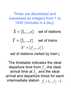
node 3. Fig.4-1 shows an illustration of the 3-node network.
Step 1:
In a certain time instance k, node 1, 2 and 3 will observe and sample its localization
information li (k ) . Further, the nodes will calculate the distance between each other
through public beacon exchange according to Eq.(4-1).
17
ADV (k ) d1,2 (k ) d1,3 (k )
Node 1
Node 2
RD d1,2 (k )
ADV (k )
Node 3
d1,2 (k ) ADV (k ) d3,1 (k )
Figure 4-1: Illustration of the 3-node network of basic protocol
d1,2 (k ) d 2,1 (k ) | l1 (k ) l2 (k ) |
d1,3 (k ) d3,1 (k ) | l1 (k ) l3 (k ) |, k (1, 2, , n)
(4-1)
Here li (k) is the quantized position for node i in time slot k. d1,2 (k) is defined as the
Reference Distance (RD). And note that distance between node 1 and 2 is identical no
matter how it is measured from node 1 or node 2 during the same time interval.
Step 2:
Node 1 will calculate the Additive Distance Value (ADV) as ADV (k ) d1,2 (k ) d1,3 (k ) and
then forward the ADV to node 3, while node 2 already know RD as d2,1 (k) .
Step 3:
When node 3 receives the ADV from node 1, it is able to estimate the RD (distance
between node 1 and node 2), which is d1,2 (k ) ADV (k ) d3,1 (k ) . Since node 2 can measure the
RD from its end, d2,1 (k ) d1,2 (k ) , the node 1, node 2 and node 3 have obtained the same
localization information RD. Therefore, the secret key can be generated collaboratively
18
through secret bit extraction (the secret bit extraction algorithm will be explained later)
based on RD.
4.2 Secret Key Generation Algorithm
Phase 1. Quantization
First, the nodes
1, 2, , m quantize the field Φ and estimate their localization information
as li (k ) , i (1, 2, , m),
k (1, 2, , n) ,
at time slot k and store them in their buffers. In this
phase, a variety of technologies for localization estimation could be utilized such as
infrared, wireless radios, ultrasound, Lidar, Radar, and so on, which make the applicability
of secret key generation over localization very robust.
Phase 2. Public Discussion
In this phase, a public discussion phase is conducted for the nodes to calculate their
relative distance as di, j (k) d j,i (k) | li (k) l j (k) | , i,
j (1, 2, , m), k (1, 2, , n)
at time slot k.
The distance between two randomly selected nodes 1 and 2 d1,2 (k) is termed as RD. Then
ADV is calculated and distributed for secret key generation based on the topology of the
wireless network. Following is the detailed protocol of public discussion based on different
topologies.
A. Star Topology
Under the circumstance that every node is within the communication range of another
wireless node, a star topology is usually formed. In this case, we can easily extend the basic
19
protocol of 3-node network to an m node wireless network. See Fig.4-2 for an illustration
of the star topology network.
1) In the star topology, node 1 and node 2 are randomly selected, while the distance
between node 1 and node 2 is termed as R RD d1,2 (k ) .
2) Node 1 is selected as the central node and it calculates the ADV for every node i other
than node 1 and node 2, where ADV ,i (k ) d1,2 (k ) d1,i (k ) ,
i (3, 4, , m) .
Node 2
estimates the RD as d 2,1 (k ) . And all other node i estimates its relative distance from
node 1 as di,1 (k) .
3) Node 1 distributes the ADV ADV ,i (k ) for each node i through the public discussion.
After node i receives the ADV ADV ,i (k ) , it can calculate the RD as d1,2 (k ) ADV ,i (k )
di ,1 (k ) . As a result, all the m nodes would obtain the RD after the public discussion.
4) Meanwhile, note that the eavesdropper E would overhear all the public discussion. In
the star topology, the public discussion is a set of ADV value for node 3, 4… m. Let
E pub (k ) be the public discussion overheard by eavesdropper E. E pub (k ) can be presented
as:
E pub (k ) [ ADV ,3 (k ), ADV ,4 (k ), , ADV ,m (k )]
[(d1,2 (k ) d1,3 (k )), (d1,2 (k ) d1,4 (k )), , (d1,2 (k ) d1,m (k ))]
20
(4-2)
Node 2
Node E
RD d1,2 (k )
Node 1
ADV ,3 (k )
ADV ,i (k ) d1,2 (k ) d1,i (k )
i (3,4, , m)
ADV ,m (k )
ADV ,4 (k )
Node 4
Node 3
d1,2 (k ) ADV ,3 (k ) d3,1 (k)
Node m
d1,2 (k ) ADV ,m (k ) dm,1 (k )
d1,2 (k ) ADV ,4 (k ) d4,1 (k )
Figure 4-2: Illustration for an m node wireless network with star topology
B. Chain Topology
For the situation that not every node is within the communication range of other wireless
nodes, however they are interconnected, a chain topology is suggested. See Fig.4-3 for an
illustration of the chain topology network.
Node E
ADV ,3 (k ) d2,1 (k ) d2,3 (k )
Node 1
ADV ,4 (k ) ADV ,3 (k ) d3,2 (k ) d3,4 (k )
Node 2
Node 3
ADV ,3 (k )
RD d1,2 (k )
ADV ,i (k ) ADV ,i 1 (k ) di ,i 1 (k ) di ,i 1 (k )
Node 4
ADV ,4 (k )
Node m
ADV ,i (k )
d1,2 (k ) ADV ,3 (k ) d3,2 (k ) d1,2 (k ) ADV ,4 (k ) d4,3 (k )
d1,2 (k ) ADV ,m (k ) dm,m 1 (k )
Figure 4-3: Illustration for an m node wireless network with chain topology
21
1) Node 1 and node 2 are randomly selected, while the distance between node 1 and
node 2 is termed as RD d1,2 (k ) .
2) Node 1 is selected as the head node and node m is selected as the tail node of the
chain topology. Node 2 calculates the ADV for node 3 as ADV ,3 (k ) d2,1 (k ) d2,3 (k ) .
Node 2 estimates the RD as d 2,1 (k ) .
3) Upon the reception of ADV ,3 (k ) , node 3 calculates the RD as d1,2 (k ) ADV ,3 (k ) d3,2 (k )
and also passes the ADV for next node 4 as ADV ,4 (k ) ADV ,3 (k ) d3,2 (k ) d3,4 (k ) .
Similarly, upon the reception of ADV ,4 (k ) , node 4 calculates RD as d1,2 (k ) ADV ,4 (k )
d4,3 (k ) and also passes ADV for next node 5 as ADV ,5 (k ) ADV ,4 (k ) d4,3 (k )
d 4,5 (k) .
4) In summary, node i i (3, 4, , m 1) estimates its relative distance from its neighbor
node i-1 and i+1 as di ,i 1 (k ) and di ,i 1 (k ) . Then, upon the reception of its ADV
ADV ,i (k ) , node i calculates the RD as d1,2 (k ) ADV ,i (k ) di ,i 1 (k ) and also passes the
ADV for next node i+1 as ADV ,i 1 (k ) ADV ,i (k ) di ,i 1 (k ) di ,i 1 (k ) . And for node m, it
only needs to calculate the RD as d1,2 (k ) ADV ,m (k ) dm,m1 (k ) .
5) Also, the eavesdropper E would overhear all the public discussion through all the
public discussion. In the chain topology, the public discussion is also a set of ADV
value for node 3, 4… m. The public discussion overheard by eavesdropper E E pub (k )
can be presented as:
22
E pub (k ) [ ADV ,3 (k ), ADV ,4 (k ), , ADV ,m ( k )]
[(d1,2 (k ) d 2,3 (k )), (d1,2 (k ) d3,4 (k )), , (d1,2 (k ) d m1,m (k ))]
(4-3)
C. Hybrid Topology
For certain circumstances like large scale wireless network, only the star and chain
topology may not be adequate for the wireless network. Under such situation, a hybrid
topology is suggested as a combination of star and chain topology. Fig.4-4 illustrates the
hybrid topology.
Node E
Node 11
Node 21
Node m1
Node 0
Node 1
Node 2
Node m
Chain
Topology
Star
Topology
Node 12
Node 22
Node m2
Figure 4-4: Illustration for wireless network with hybrid topology
In the hybrid topology shown in Fig.4-4, node 0 is the head node of the hybrid topology.
Node 1, 11, 12 form a star topology, as well as node 2, 21, 22 through node m, m1, m2.
Meanwhile, node 0, node 1 through node m form a chain topology. In such wireless
network, some nodes are outside the communication range of other nodes so that the star
topology is not adequate. Further, a chain cannot form a Hamiltonian path [24] in the
wireless network so that the chain topology is not enough as well. Here the Hamiltonian
23
path is a path that visits each node in the wireless network exactly once. Therefore, a
combination of star and chain topology – the hybrid topology is suggested in such situation.
1) In the hybrid topology, node 0 and node 1 is randomly selected while the distance
between node 0 and node 1 is termed as RD d0,1 (k ) .
2) The nodes on the chain except head node 0 (node 1,2,…,m) is selected as the central
node for each star. Further, central node 1 needs to calculate and forward two ADV.
One ADV is for every other nodes in the 1st star (node 11, 12,……1m ), assuming there
1
are m1 nodes in the 1st star. Here ADV ,1j (k ) d1,0 (k ) d1,1j (k ), j (1,2, , m1 ) . Node 1j then
could calculate the RD as d0,1 (k ) ADV ,1j (k ) d1j ,1 (k ) . The other ADV is for the next
central node in the chain, node 2. Here ADV ,2 (k ) d1,0 (k ) d1,2 (k ) .
3) Upon the reception of ADV ,2 (k ) at node 2. Node 2 can calculate the RD as
d0,1 (k ) ADV ,2 (k ) d2,1 (k ) . Node 2 also needs to calculate and forward two ADV. One
ADV is for every other nodes in the 2nd star (node 21,22,…… 2m ), assuming there are
2
m2 nodes in the 2nd star. Here
ADV ,2 j (k ) ADV ,2 (k ) d2,1 (k ) d2,2 j (k ), j (1,2, , m2 ) . Node
2j then could calculate the RD as d0,1 (k ) ADV ,2 j (k ) d2 j ,2 (k ) . The other ADV is for the
next central node in the chain, node 3. Here ADV ,3 (k ) ADV ,2 (k ) d2,1 (k ) d2,3 (k ) .
4) Accordingly, node i, i (2,3, , m) calculates the RD as d0,1 (k ) ADV ,i (k ) di,i 1 (k ) upon
its ADV reception of ADV ,i (k ) . Node i also needs to calculate and forward two ADV.
One ADV is for every other nodes in the ith star (node i1, i2,…… i mi ), assuming there
24
are mi nodes in the ith star. Here ADV ,i j (k ) ADV ,i (k ) di,i 1 (k ) di,i j (k ) , j (1,2, , mi ) .
And node ij then could calculate the RD as d0,1 (k ) ADV ,i j (k ) di j ,i (k ) . The other ADV is
for the next central node in the chain, node i+1. Here ADV ,i 1 (k ) ADV ,i (k ) di,i 1 (k )
di,i 1 (k ) . Especially for node m, it does not need to calculate ADV for the next central
node.
5) Also, the eavesdropper E would overhear all the public discussion through all the
public discussion. The public discussion overheard by eavesdropper E E pub (k ) can be
presented as the combination of all ADV information including star and chain:
E pub (k ) [ ADV ,11 ( k ), , ADV ,1m1 ( k ), ADV ,21 ( k ), , ADV ,2m2 ( k ), , ADV ,m1 ( k ), , ADV ,mmm ( k )],
[ ADV ,2 (k ), ADV ,3 ( k ), , ADV ,m ( k )]
[(d 0,1 (k ) d1,11 (k )), , (d 0,1 (k ) d1,1m1 ( k )), ( d 0,1 ( k ) d 2,21 ( k )), ,
(d 0,1 (k ) d 2,2m2 (k )), , (d 0,1 (k ) d m,m1 (k )), , ( d 0,1 ( k ) d m,mmm ( k ))],
(4-4)
[(d 0,1 (k ) d1,2 (k )), ( d 0,1 ( k ) d 2,3 ( k )), , ( d 0,1 ( k ) d m 1,m ( k ))]
Phase 3. Secret Bit Extraction
In this phase, an r bit secret key is extracted based on the RD received by the legitimate
nodes in each time slot through three different secret bit extraction steps. Here the bit
number r can be selected to give an adequate length to the secret key. For a single time slot
r bits secret key is generated and there are totally n time slots, therefore the final generated
secret key would have a length of n r bits.
Let the RD calculated by node i be RDi ,k d1,2@i (k ), i (1, 2, , m), k (1, 2, , n) , where
d1,2@ i (k ) means the d1,2 value calculated by the node i at time slot k, and for every node 1
25
to node m, n time slot RD measurements are made as RDi ,k . Three types of bit extraction
steps are utilized for each RD measurement collaboratively to achieve an r bit secret key
Si ,k ( ), (1, 2, , r)
for each time slot k. Let the mean value of RDi ,k be
mi
RD
k
and
i ,k
n
F ( RDi ,k ) be the cumulative distribution function of RDi ,k . The following secret bit
determination algorithm presents the proposed secret bit extraction protocol for Si ,k ( ) .
For a set of RD measurements RDi,k , i (1, 2, , m), k (1, 2, , n)
0, if RDi ,k mi 0
1, if RDi ,k mi 0
i)
Si ,k (1)
ii)
Si ,k (2)
iii)
Si ,k ( ), (3,4, , r ) , here 2r-2 quantization levels are used where
(4-5)
0, if RDi ,k RDi ,k 1 0
1, if RDi ,k RDi ,k 1 0
(4-6)
(4-7)
q0 min( RDi,k ), q 2r2 max( RDi ,k )
and qu F 1 ( ur 2 ), u 1, 2, , 2r 2 1
2
1
Here qu F (
(4-8)
u
) is to make sure that qu is selected based on the same
2r 2
distribution function of RDi ,k . The ‘u’th quantization bin is defined as the interval
[qu 1 ,qu ] , and Gray coding is employed for bit extraction.
1) For a single observed RDi ,k d1,2 , the value is mainly decided by the distance between
node 1 and node 2. Let the threshold based on RDi ,k minus the mean distance
26
mi
could reduce the influence of node distance and amplify the randomness of the RD
in step i.
2) For step ii, the evaluation of RDi,k RDi,k 1 implies the moving trend of node 1 and
node 2.
3) Step iii, secret key bit number r is selected by the user in order to give an adequate
length to the generated secret key Si ,k ( ) . By increasing the secret key bit number r,
the secrecy privilege of the legitimate nodes over the eavesdropper is increased since
it is harder for the eavesdropper to decipher the same secret key. However, it will
also make the secret bit extraction algorithm more vulnerable to the noise and thus
increase the bit mismatch rate of the legitimate nodes. In this thesis, r is selected as
4 considering this tradeoff and the simplicity for simulation.
4) Finally, by combining all the Si ,k ( ) extracted from n time slots, node i is able to
generate the secret key as Si ( ) , (1, 2, , n*r ) . Since RD is identical for each node,
all the m nodes are then able to agree on a synchronized secret key Si ( ) .
Example: Let the RD of {98m, 99m, 100m, 101m, 102m, 103m} is received in n = 6
time slots at node i. RD follows a uniform distribution that the probability for each RD
value is identical. Based on each received RD value, an r = 4 bit secret key needs to be
extracted. Here the mean value of RD is 100.50. Since RD is uniformly distributed, the 2r2
=4 quantization bins are [98, 99.25], [99.25, 100.50], [100.50, 101.75], [101.75, 103]. The
corresponding 2 bit Gray code is [00, 01, 11, 10].
27
1) For time slot k = 1, RDi,1 98 is less than mean value mi = 100.50, therefore Si ,1 (1) 0 .
Since RDi ,1 is the first RD value, Si,1 (2) 0 . RDi ,1 falls in the first quantization bin [98,
99.25] so that Si,1 (3,4) 00 . Thus, the generated secret key Si,1 ( ) for time slot 1 is 0000.
2) For time slot k = 2, RDi ,2 99 is less than mean value mi = 100.50, therefore Si ,2 (1) 0 .
Since RDi ,2 RDi ,1 , Si ,2 (2) 1 . RDi ,2 falls in the first quantization bin [98, 99.25] and
Si,2 (3,4) 00 . Thus, the generated secret key Si ,2 ( ) for time slot 2 is 0100.
3) For time slot k = 3, RDi ,3 100 is less than mean value mi = 100.50, therefore Si ,3 (1) 0 .
Since RDi ,3 RDi ,2 , Si ,3 (2) 1 . RDi ,3 falls in the second quantization bin [99.25, 100.50]
and Si,3 (3,4) 01 . Thus, the generated secret key Si ,3 ( ) for time slot 3 is 0101.
4) Repeat the previous procedure for each time slot and combine all the Si ,k ( ) together
and then node i could generate the secret key as “0000 0100 0101 1111 1110 1110”.
In summary, the proposed secret key generation algorithm is presented in this chapter,
including m node wireless network topology design and secret bit extraction method. Later,
the maximum secret key generation rate for the proposed algorithm will be derived in
Chapter 5.
28
Chapter 5
Theoretical Analysis for MSR
A theoretical analysis for the Maximum achievable Secret key generation Rate (MSR)
is conducted in this chapter. Based on different network topology, the MSR is different
from each other. Therefore, the theoretical analysis is conducted based on star, chain and
hybrid topology respectively.
5.1 Star Topology Based MSR
Following is a brief review of the star topology:
Step 1: Node 1 and node 2 is randomly selected to get Reference Distance (RD) as
RD d1,2 (k ) .
Node 1 and node 2 estimate RD as d1,2 (k ) and d2,1 (k ) respectively.
Step 2: Node 1 publishes the ADV to node i, i (3, 4, , m) as ADV ,i (k ) d1,2 (k ) d1,i (k ) .
Node i calculates distance from node 1 as di ,1 (k ) .
Step 3: Node i estimates RD as d1,2 (k ) ADV ,i (k ) di ,1 (k ) .
Step 4: Secret bit extraction based on RD is processed to generate final secret key.
According to the theoretical analysis proposed by Maurer and other researchers in [6-8],
secret key generation rate is the mutual information between two nodes. Since they only
29
propose the MSR based on 3-node
network,
the
mutual
Node 2
information
between central node 1 and all other
node
i
including
Node E
Node 1
eavesdropper,
i (2,3, , m,e) should be examined
Node 3
Node 4
Node m
for the star topology wireless network.
Figure 5-1: Brief on star topology
For simplicity, let’s assume that all
information sequences are independent identically distributed (i.i.d). Let any random
sequence z(k) through time slot 1, 2, …, n be Z [z(1), z(2), , z(n)] . Then the localization
information sequence acquired for node 1 should be D1 [D1,2 , D1,3 , , D1,m ] [d1,2 (1), , d1,2 (n), ,
d1,m (1), , d1,m (n)] . For node 2, RD d1,2 d2,1 is given. All other node i, i (3, 4, , m) have
to calculate RD through ADV public discussion and may suffer from noise or other
distractions. Therefore, secret key generation rate for node 2 is higher than any other nodes
and the MSR is based on the mutual information between node 1 and node i,
i (3, 4, , m) . Let’s consider node i, i (3, 4, , m) . Node 1 broadcasts the ADV to all
nodes with ADV sequence in the public discussion. Thus node i overhear all ADV public
discussion as E pub (k ) [ ADV ,3 (k ) , ADV ,4 (k ), , ADV ,m (k )] [d1,2 (k ) d1,3 (k ), d1,2 (k ) d1,4 (k ), ,
d1,2 (k ) d1,m (k )] and E pub [ E pub (1) , E pub (2), , E pub (n)] . Node i then estimate the RD
with its own localization sequence Di ,1 and the ADV sequence E pub . Therefore the
information for node i is the joint information of [Di ,1 , E pub ] . The ADV sequence E pub is
also overheard by eavesdropper node e. Here, node e is considered to overhear the
30
localization information as well. Let the localization information acquired by node e be
De [De,1 , De,2 , , De,m ] . Next, the MSR is derived as
slot
n ,
T
. A same approach is made as time
which yields MSR, under large enough time scale.
MSR (bits/sample) for node i can be presented as:
Ri lim
n
1
I(D1; Di,1 , E pub )
n
(5-1)
MSR for the m node wireless network is limited by the worst node (eg. the node has
higher noise interference than others), which can be presented as:
Rnode min Ri
3i m
(5-2)
Considering the presence of eavesdropper, the final MSR can be presented as the
information obtained by nodes minus the information obtained by eavesdroppers:
R final Rnode lim
n
1
I(D1 ; De , E pub )
n
(5-3)
Since the i.i.d assumption has been made for all information sequence, Ri for any node
i (3, 4, , m) is identical. Therefore, an arbitrary node 3 is considered for MSR. Further,
based on the i.i.d assumption and the simplicity of derivation, a single time slot is
considered. Based on former assumptions, the final MSR can be expanded as:
R final I([d1,2 , d1,3 , , d1,m ]; d3,1 , E pub ) I([d1,2 , d1,3 , , d1,m ];[d e,1 , d e,2 , , d e,m ], E pub ) …………..(5-4)
I([d1,2 , d1,3 , , d1,m ]; E pub ) I([d1,2 , d1,3 , , d1,m ]; d3,1 | E pub )
I([d1,2 , d1,3 , , d1,m ]; E pub ) I([d1,2 , d1,3 , , d1,m ];[de,1 , d e,2 , , d e,m ]| E pub ) ………….....(5-5)
I([d1,2 , d1,3 , , d1,m ]; d3,1 | E pub ) …………………………………………..………..(5-6)
= I(d1,2 ; d3,1 | E pub ) I([d1,3 , , d1,m ]; d3,1 | d1,2 , E pub ]) …………………………………..(5-7)
31
= I(d1,2 ; d3,1 | E pub )
……………………………………………………………..….(5-8)
= h(d1,2 | E pub ) h(d1,2 | d3,1 , E pub )
……………………………….………………….(5-9)
= h(E pub | d1,2 ) h( E pub ) h(d1,2 ) (h(d3,1 , E pub | d1,2 ) h(d3,1 , E pub ) h(d1,2 )) ………….(5-10)
= h([d1,2 d1,3 , d1,2 d1,4 , , d1,2 d1,m ] | d1,2 ) h([d1,2 d1,3 , d1,2 d1,4 , , d1,2 d1,m ]) ….(5-11)
h(d3,1 ,[d1,2 d1,3 , d1,2 d1,4 , , d1,2 d1,m ] | d1,2 ) h(d3,1 ,[d1,2 d1,3 , d1,2 d1,4 , , d1,2 d1,m ])
= h([d1,3 , d1,4 , , d1,m ]) h([d1,2 d1,3 , d1,2 d1,4 , , d1,2 d1,m ])
h(d3,1 , d1,3 , d1,4 , , d1,m ) h(d3,1 , d1,2 d1,3 , d1,2 d1,4 , , d1,2 d1,m ) ……………...…(5-12)
Here, Eq.(5-5) follows Eq.(3-9) such that I (X; Y, Z) I(X; Z) I (X; Y | Z) . Eq.(5-6)
is due to the i.i.d assumption, di, j is independent from d e,i . Eq.(5-7) follows the chain rule.
Eq.(5-8) is because, given that d1,2 and E pub , d1,3 , , d1,m are determined, the entropy is 0.
Eq.(5-9) follows Eq.(3-8) since I (X;Y | Z) H(X | Z) H(X | Y, Z) . Eq.(5-10) follows
Eq.(3-10) since H (Y | X ) H (X | Y ) H(X) H (Y) . Eq.(5-11) is the expansion of Eq.(510). Eq.(5-12) is because, for given d1,2 , the randomness in [d1,2 d1,3 , d1,2 d1,4 , , d1,2 d1,m ]
can be simply presented as [d1,3 , d1,4 , , d1,m ] .
Next, the MSR is further estimated through Gaussian distribution assumption that all
observations of distance terms are considered as i.i.d Gaussian processes. In real wireless
communication environment, the distance information can be presented as the sum of node
`
distance and noise: di, j (k) d i, j (k) wi, j (k) , where wi, j (k) is an additive Gaussian noise.
The distance measured at both end i and j should be identical, so d `i, j (k) d `j,i (k) . However
the noise at different node is uncorrelated, hence wi, j (k) and wj,i (k) are independent. Since
the entropy of Gaussian distribution d `i, j (k) is only a function of its variance d2 as is defined
in Eq.(3-11) that h(d `i, j (k)) 1 ln(2 e d 2 ) , the mean value does not affect the MSR
2
32
estimation and can be ignored. Here the mean value of d `i, j (k) is defined as the average
distance between node i and j through the secret key generation process (for n time slots).
The variance d2 can be considered as the variation of distance due to relative movement of
the nodes involved. Since the randomness only lies in the movement of the nodes, the mean
value can be considered as 0. Therefore d `i, j (k) can be considered as i.i.d processes with 0
mean and d2 variance. Let the additive Gaussian noise wi, j (k) also be i.i.d processes with 0
mean and variance w2 . Then
d2
is defined as the signal-to-noise ratio (SNR).
w2
The four components of MSR derived above can be estimated one by one as:
i): [d1,3 , d1,4 , , d1,m ] ~ N (0, 1 ) , here the covariance matrix 1 is an (m-2) (m-2)
matrix that
1 (i, i) cov(d1,i , d1,i ) d2 w2 d2 (1 1 )
1 (i, j ) cov(d1,i , d1, j ) 0
(5-13)
i,j (1,2, ,m-2) and i j
det( 1 )=( d2 (1 1 ))(m 2)
det( 1 ) can be calculated using eq.(3-13).
ii): [d1,2 d1,3 , d1,2 d1,4 , , d1,2 d1,m ] ~ N (0, 2 ) , here the covariance matrix 2 is an
(m-2) (m-2) matrix that
2 (i, i ) cov(d1,2 d1,i , d1,2 d1,i ) cov(d1,2 , d1,2 d1,i ) cov( d1,i , d1,2 d1, j )
cov( d1,2 , d1,2 ) cov( d1,2 , d1,i ) cov( d1,i , d1,2 ) cov( d1,i , d1,i )
cov( d1,2 , d1,2 ) cov( d1,i , d1,i ) 2( d2 w2 ) 2 d2 (1 1 )
33
2 (i, j ) cov(d1,2 d1,i , d1,2 d1, j ) cov(d1,2 , d1,2 d1,i ) cov(d1,i , d1,2 d1, j )
cov( d1,2 , d1,2 ) cov( d1,2 , d1,i ) cov( d1,i , d1,2 ) cov( d1,i , d1, j ) cov( d1,2 , d1,2 )
d2 w2 d2 (1 1 ),
i,j (1,2, ,m-2) and i j
det( 2 )=(m 1)( (1 ))
2
d
1
(5-14)
(m 2)
det( 2 ) can be calculated using eq.(3-13).
iii): [d3,1 , d1,3 , d1,4 , , d1,m ] ~ N (0, 3 ) , here the covariance matrix 3 is an (m-1) (m1) matrix that the right bottom portion of the matrix [2,m-1] [2,m-1] is identical to
1 and the first column and first row is as follow:
3 (1,1) cov( d3,1 , d3,1 ) ( d2 w2 ) d2 (1 1 )
3 (1, 2) 3 (2,1) cov( d3,1 , d1,3 ) cov( d `3,1 w3,1 , d `1,3 w1,3 )
cov( d `3,1 , d `1,3 ) cov( w3,1 , w1,3 ) cov( d `3,1 , d `1,3 ) d2
d `1,3 d `3,1 and w1,3 is independent from w3,1
d2 w2
d2
0
2
2
2
d w
0
d
2
det( 3 )=det
d w2
0
0
0
0
0
0
0
2
2
d w
0
(5-15)
d2 w2
d2
0
0
0
2
2
2
d w
0
0
0 d w2
( d2 w2 ) |
d2 |
2
2
d w
0
0
0
0
d2 w2
0
2
2
2
2 (m 2)
4
=( d w )( d w )
d |
2
2
0
d
w
=( d2 w2 ) (m 1) d4 ( d2 w2 )(m 3) ( d2 w2 )(m 1) (1
=( d2 (1 1 ))(m 1) (1
1
(1 1 ) 2
)
det( 3 ) is calculated using Laplace expansion.
34
d4
)
( d2 w2 ) 2
0
2
2
d w
0
iv): [d3,1 , d1,2 d1,3 , d1,2 d1,4 , , d1,2 d1,m ] ~ N (0, 4 ) , here the covariance matrix 4
is an (m-1) (m-1) matrix that the right bottom portion of the matrix [2,m-1] [2,m1] is identical to 2 and the first column and first row is as follow:
4 (1,1) cov(d3,1 , d3,1 ) ( d2 w2 ) d2 (1 1 )
4 (1, 2) 4 (2,1) cov( d3,1 , d1,2 d1,3 ) cov( d3,1 , d1,2 ) cov( d3,1 , d1,3 ) d2
d2 w2
2
d
det( 4 )=det 0
0
d2
0
2
w
2
w
d2 w2
2
d
2
d
2( d2 w2 )
0
2( )
2( )
2
d
2
d
2
w
2
w
d2 w2
2
d
2
d
(5-16)
2
w
2
w
2( d2 w2 ) d2 w2
d2
d2 w2
d2 w2
2
2
2
2
2
2
w
2( d w )
d w
0 2( d2 w2 )
( d2 w2 ) | d
d2 |
2
2
2
2
2
2
2( d w )
d w
d2 w2
d w
0
2( d2 w2 )
d2 w2
=( d2 w2 )(m 1)( d2 w2 ) (m 2) d4 |
2
2
d2 w2
2(
)
d
w
=(m 1)( d2 w2 ) (m 1) d4 (m 2)( d2 w2 )(m 3) ( d2 w2 )(m 1) (m 1
=( d2 (1 1 ))(m 1) (m 1
d2 w2
d2 w2
2( )
2
d
2
w
d4 (m 2)
)
( d2 w2 ) 2
m 2
)
(1 1 ) 2
det( 4 ) is calculated using Laplace expansion.
Based on Eq.(3-12), h 1 ln{(2 e)m | |} , the MSR of star topology with Gaussian
2
distribution estimation is:
1
1
R final ln{(2 e) m 2 ( d2 (1 1 )) m 2 } ln{(2 e) m 2 (m 1)( d2 (1 1 )) m 2 }
2
2
1
1
1
m 2
ln{(2 e) m 2 ( d2 (1 1 )) m 1 (1
)} ln{(2 e) m 2 ( d2 (1 1 )) m 1 (m 1
)}
1 2
2
(1 )
2
(1 1 ) 2
1
1
1
1
m 2
ln(m 1) ln(1
) ln(m 1
)
1 2
2
2
(1 )
2
(1 1 ) 2
(5-17)
1
1
ln(1
)
1 2
2
(m 1)((1 ) 1)
Here m is the total number of nodes in the star topology and d2 is the SNR.
w
2
35
5.2 Chain Topology Based MSR
Let’s make a brief by reviewing the concept of chain topology:
Step 1: Node 1 and node 2 is randomly selected that RD d1,2 (k ) , k (1, 2, , n) .
Step 2: Node 2 passes the ADV ADV ,3 (k ) d2,1 (k ) d2,3 (k ) to node 3. Node i, i (3, 4, , m)
calculates distance from neighbor nodes as di ,i 1 (k ), di,i 1 (k ) .
Step 3: Node i, i (3, 4, , m) estimates RD as d1,2 (k ) ADV ,i (k ) di,i 1 (k ) . Node i also passes
node i+1 the ADV, ADV ,i 1 (k ) ADV ,i (k ) di,i 1 (k ) di,i 1 (k ) .
Node m only estimates RD as d1,2 (k ) ADV ,m (k ) dm,m1 (k ) .
Step 4: Secret bit extraction based on RD is processed to generate final secret key.
Node E
Node 1
Node 2
Node 3
Node 4
Node m
Figure 5-2: Schematic diagram of chain topology
Similar to the star topology, the mutual information between head node 1 and all other
node i, i (2,3, ,m,e) should be examined for the chain topology wireless network. The i.i.d
assumption is also made for simplicity. The localization information sequence acquired for
node 1 should be D1,2 [d1,2 (1), d1,2 (2), , d1,2 (n)] . Likewise, secret key generation rate for
node 2 is faster than other nodes since RD is given for node 2. Therefore, the MSR is also
36
based on the mutual information between node 1 and the nodes other than node 1 and node
2. Let’s consider node i, i (3,4, ,m) . The localization information node i acquires should
be Di,i 1 and Di ,i1 . For tail node m, the localization information should be Dm,m 1 . The ADV
for node i is E pub,i [ ADV ,i (1), ADV ,i (2), , ADV ,i (n)] [d1,2 (1) di 1,i (1), d1,2 (2) di 1,i (2), , d1,2 (n) di 1,i (n)]
and E pub,i1 . Therefore the information for node i can be written as [Di,i 1 , Di,i 1 , E pub,i , E pub,i 1 ]
and for node m is [Dm,m1, E pub,m ] . For the eavesdropper e, the localization information is
De [De,1 , De,2 , , De,m ]
. Eavesdropper e is also assumed to overhear all public ADV
information, therefore the ADV public discussion for node e is Epub (k ) [ ADV ,3 (k ), ADV ,4 (k ), ,
ADV ,m (k )] [d1,2 (k ) d2,3 (k ), d1,2 (k ) d3,4 (k ), , d1,2 (k ) dm 1,m (k )] and E pub [ E pub (1), E pub (2), , E pub (n)] .
Similarly, the MSR is derived as
n
MSR (bits/sample) for node i, i (3, 4, , m1) in chain topology can now be presented
as:
Ri lim
n
1
I(D1,2 ; Di 1,i , Di ,i 1 , E pub ,i , E pub ,i 1 )
n
(5-18)
Also MSR for node m can be presented as:
Rm lim
n
1
I(D1,2 ; Dm,m 1 , E pub,m )
n
(5-19)
Since MSR for the m node wireless network then can be determined by
Rnode min Ri
3i m
37
(5-20)
And node m has less information than other nodes and node m is the farthest end node
of the chain, we can predict that Rm Ri , therefore:
Rnode Rm
(5-21)
Considering the presence of eavesdropper, the final MSR can be presented as the
information obtained by nodes minus the information obtained by eavesdroppers:
R final Rnode lim
n
1
1
I(D1,2 ; De , E pub ) Rm lim I(D1,2 ; De , E pub )
n
n
n
(5-22)
Similarly, based on the i.i.d assumption for all information sequence, the final MSR can
be simplified by dropping time indices as:
R final I(d1,2 ; d m,m 1 , E pub,m ) I(d1,2 ;[d e,1 , d e,2 , , d e,m ], E pub ) ……………………………………(5-23)
I(d1,2 ; E pub,m ) I(d1,2 ; d m,m 1 | E pub,m )
I(d1,2 ; E pub ) I(d1,2 ;[d e,1 , d e,2 , , d e,m ]| E pub ) …………………………………………(5-24)
I(d1,2 ; E pub,m ) (I(d1,2 ; E pub,m ) I(d1,2 ;( E pub,3 , E pub,4 , , E pub,m 1 ) | E pub,m )) I(d1,2 ; d m,m 1 | E pub,m ) …(5-25)
= h(d1,2 | E pub,m ) h(d1,2 | ( E pub,3 , E pub,4 , , E pub,m 1 ), E pub,m )
.
h(d1,2 | E pub,m ) h(d1,2 | d m,m 1 , E pub,m ) ……………………………………………….(5-26)
= h(( E pub,3 , E pub,4 , , E pub,m 1 ), E pub,m | d1,2 ) h(( E pub,3 , E pub,4 , , E pub,m 1 ), E pub,m ) h(d1,2 )
(h(d m,m 1 , E pub,m | d1,2 ) h(d m,m 1 , E pub,m ) h(d1,2 )) …………………………………….(5-27)
= h([d1,2 d 2,3 , d1,2 d3,4 , , d1,2 d m 2,m 1 ], d1,2 d m 1,m | d1,2 )
h([d1,2 d 2,3 , d1,2 d3,4 , , d1,2 d m 2,m 1 ], d1,2 d m 1,m )
h(d m,m 1 , d1,2 d m 1,m | d1,2 ) h(d m,m 1 , d1,2 d m 1,m ) ……………….…………………...(5-28)
= h (d 2,3 , d3,4 , , d m 1,m ) h([d1,2 d 2,3 , d1,2 d3,4 , , d1,2 d m 1,m ])
h(d m,m 1 , d m 1,m ) h(d m,m 1 , d1,2 d m 1,m )
……………………….……………………(5-29)
Here, Eq.(5-24) follows Eq.(3-9) I (X; Y, Z) I(X; Z) I (X; Y | Z) . Eq.(5-25) follows
Eq.(3-9) while considering E pub ( E pub,3 , E pub,4 , , E pub,m 1 ), E pub,m . Also based on i.i.d
38
assumption, di, j is independent from de,i . Eq.(5-26) follows Eq.(3-8) since I (X; Y | Z)
H(X | Z) H(X | Y, Z) . Eq.(5-27) follows Eq.(3-10), H (Y | X ) H (X | Y ) H(X)
H (Y) . Eq.(5-28) is the expansion of Eq.(5-27). Eq.(5-29) is because, given d1,2 , the
randomness in [d1,2 d2,3 , d1,2 d3,4 , , d1,2 dm 1,m ] can be simply presented by [d2,3 , d3,4 , , dm1,m ] .
Similarly, the MSR for chain topology is further estimated through Gaussian distribution.
Same assumption has been made for the distance and noise signal.
The four components of MSR derived above can be estimated one by one as:
i): [d2,3 , d3,4 , , dm 1,m ] ~ N (0, 1 ) , here covariance matrix 1 is (m-2) (m-2) matrix that
1 (i, i) cov(di 1,i , di 1,i ) d2 w2 d2 (1 1 )
1 (i, j ) cov(di 1,i , d j 1, j ) 0
i,j (1,2, ,m-2) and i j
(5-30)
det( 1 )=( d2 (1 1 )) (m 2)
det( 1 ) can be calculated using eq.(3-13).
ii): [d1,2 d2,3 , d1,2 d3,4 , , d1,2 dm 1,m ] ~ N (0, 2 ) , here the covariance matrix 2 is an (m2) (m-2) matrix that
2 (i,i) cov( d1,2 di 1,i , d1,2 di 1,i ) cov(d1,2 , d1,2 d i 1,i ) cov( d i 1,i , d1,2 d i 1, j )
cov( d1,2 , d1,2 ) cov( d1,2 , di 1,i ) cov( di 1,i , d1,2 ) cov( d i 1,i , d i 1,i )
cov( d1,2 , d1,2 ) cov( di 1,i , di 1,i ) 2( d2 w2 ) 2 d2 (1 1 )
1 (i, j) cov(d1,2 di 1,i , d1,2 d j 1, j ) cov(d1,2 , d1,2 d j 1,i ) cov( d i 1,i , d1,2 d j 1, j )
cov( d1,2 , d1,2 ) cov( d1,2 , di 1,i ) cov( di 1,i , d1,2 ) cov( d i 1,i , d j 1, j )
cov(d1,2 , d1,2 ) d2 w2 d2 (1 1 ),
i,j (1,2, ,m-2) and i j
det( 2 )=(m 1)( d2 (1 1 )) (m 2)
det( 2 ) can be calculated using eq.(3-13).
39
(5-31)
iii): [dm,m1, dm1,m ] ~ N (0, 3 ) , here the covariance matrix 3 is as follow:
d2 (1 1 )
d2
3
2
2
1
d
d (1 )
where
3 (1,1) cov( d m,m 1 , d m,m 1 ) ( d2 w2 ) d2 (1 1 ) 3 (2, 2)
3 (1, 2) 3 (2,1) cov( d m,m 1 , d m 1,m ) cov( d `m,m 1 wm,m 1 , d `m 1,m wm 1,m )
(5-32)
cov( d `m,m 1 , d `m 1,m ) cov( wm,m 1 , wm 1,m ) cov(d `m,m 1 , d `m 1,m ) d2
d `m,m 1 d `m 1,m and wm,m 1 is independent from wm 1,m
det(3 ) ( d2 (1 1 )) 2 d4 d4 ((1 1 ) 2 1)
iv): [dm,m1 , d1,2 dm1,m ] ~ N (0, 4 ) , here the covariance matrix 4 is as follow:
2 (1 1 )
d2
4 d 2
1
2
d
2 d (1 )
where
4 (1,1) cov(d m,m 1 , d m 1,m ) ( d2 w2 ) d2 (1 1 )
4 (2, 2) cov(d1,2 d m 1,m , d1,2 d m 1,m ) 2( d2 w2 ) 2 d2 (1 1 )
(5-33)
4 (1, 2) 3 (2,1) cov( d m,m 1 , d1,2 d m 1,m )
cov(d m,m 1 , d1,2 ) cov(d m,m 1 , d m 1,m ) cov(d m,m 1 , d m 1,m ) d2
det(3 ) 2( d2 (1 1 )) 2 d4 d4 (2(1 1 ) 2 1)
Based on Eq.(3-12) that h 1 ln{(2 e)m | |} , the chain topology MSR with Gaussian
2
distribution estimation is:
1
1
R final ln{(2 e) m 2 ( d2 (1 1 )) m 2 } ln{(2 e) m 2 (m 1)( d2 (1 1 )) m 2 }
2
2
1
1
ln{(2 e) m 2 d4 ((1 1 ) 2 1)} ln{(2 e) m 2 d4 (2(1 1 ) 2 1)}
2
2
1
1
1
1 2
ln(m 1) ln((1 ) 1) ln(2(1 1 ) 2 1)
2
2
2
1
2(1 1 ) 2 1
ln(
)
2 (m 1)((1 1 ) 2 1)
(5-34)
Here m is the total number of nodes in the chain topology and d2 is the SNR.
w
2
40
5.3 Hybrid Topology Based MSR
For given hybrid topology depicted in Fig.5-3, a brief review can be summarized as:
Node E
Node 11
Node 21
Node m1
Node 0
Node 1
Node 2
Node m
Chain
Topology
Star
Topology
Node 12
Node 22
Node m2
Figure 5-3: Scenario of hybrid topology
Step 1: Node 0 and node 1 is randomly selected so that RD d0,1 (k ) ,
k (1, 2, , n) .
Step 2: Central node 1 publishes ADV to every other nodes in the 1st star where
ADV ,1j (k ) d1,0 (k ) d1,1j (k ), j (1, 2, , m1 ) . Node 1j estimates RD as d0,1 (k ) ADV ,1j (k )
d1 j ,1 (k ) . Central node 1 also forwards ADV to the next node in the chain, node
2, where ADV ,2 (k ) d1,0 (k ) d1,2 (k )
Step 3: Central node i (except node 1), i (2,3, , m) estimates RD as d0,1 (k ) ADV ,i (k )
di,i 1 (k ) . Central node i publishes ADV to every other nodes in the ith star
where ADV ,i (k ) ADV ,i (k ) di,i 1 (k ) di,i (k ), j (1,2, , mi ) . Node ij estimates RD as
j
j
41
d0,1 (k ) ADV ,i j (k ) di j ,i (k ) . Central node i also forwards ADV to the next node in
the chain, node i+1, where ADV ,i 1 (k ) ADV ,i (k ) di,i 1 (k ) di,i 1 (k )
Node m does not need to calculate ADV for the next central node.
Step 4: Secret bit extraction based on RD is processed to generate final secret key.
Like the theoretical analysis of star and chain topologies, the mutual information
between head node 0 and all other nodes in the wireless network should be examined. The
i.i.d assumption is also made for simplicity. The localization information sequence
acquired for node 0 should be D0,1 . According to the theoretical analysis of star topology,
the central node would have a better secret key rate than other nodes in the same star. This
is actually because central node has more information than the other nodes. Therefore its
mutual information with node 0 will be larger as well. Additionally, based on the i.i.d
assumption, the secret key rate Ri , i (1, 2, , m) for the ith star can be derived by considering
an arbitrary node ij j (1, 2, , mi ) in the star except the central node i. The localization
information for node ij would be Di ,i . ADV sequence for node ij is E pub,i
j
st
star
(k )
and
[ ADV ,i1 (k ), ADV ,i2 (k ), , ADV ,imi (k )] [d0,1 (k ) di ,i1 (k ), d0,1 (k ) di ,i2 (k ), , d0,1 (k ) di ,imi (k )]
j
E pub,ith star [ E pub,ist star (1), E pub,ist star (2), , E pub,ist star (n)] . Therefore the information for node i is the
joint information of [Di ,i , E pub,i
j
th
star
] . In order to prove that the central node has a better secret
key rate than other nodes in the same star, the localization and ADV information for node
i
is
listed
below.
Di [Di,i 1 , Di,i 1 , Di,i1 , , Di,imi ]
The
localization
information
for
node
i
would
be
and E pub,i (k ) [ ADV ,i (k ), ADV ,i 1 (k ), ADV ,i (k ), ADV ,i (k ), , ADV ,i (k )] .
1
42
2
mi
It is obvious that both Di and E pub,i are larger than Di j ,i and E pub,i
th
. Therefore central
star
node has more information and better secret key rate than node ij. For eavesdropper e, the
localization information acquired by e is De [De,1 , , De,1 , , De,m , , De,m ],[De,0 , De,1, , De,m ] .
m1
1
mm
1
Eavesdropper e is assumed to overhear all the public ADV information, thus the ADV
public discussion for node e is E pub (k ) [ ADV ,1 (k ), , ADV ,1 (k ), ADV ,2 (k ), , ADV ,2 (k )
1
m1
m2
1
, , ADV ,m1 (k ), , ADV ,mmm (k )],[ ADV ,2 (k ), ADV ,3 (k ), , ADV ,m (k )] [(d0,1 (k ) d1,11 (k )), ,
(d0,1 (k ) d1,1m1 (k )), (d0,1 (k ) d2,21 (k )), , (d0,1 (k ) d 2,2m2 (k )), , (d0,1 (k ) d m,m1 (k )), , (
and
d0,1 (k ) dm,mmm (k ))],[(d0,1 (k ) d1,2 (k )), (d0,1 (k ) d 2,3 (k )), , (d0,1 (k ) d m1,m (k ))]
E pub [ E pub (1), E pub (2), , E pub (n)] . Similarly, the MSR is derived as n
MSR (bits/sample) for the ith star i (1, 2, , m), j (1, 2, , mi ) can be presented as:
Ri lim
n
1
I(D0,1 ; Di j ,i , E pub ,ith star )
n
(5-35)
MSR for the M node wireless network then can be determined by
(5-36)
Rnode min Ri
1i M
Here Ri is proportional to mi . This is because, higher mi means more nodes in the ith star
and thus more ADV information ( E pub,i
th
star
) is published through the public discussion.
Node ij in the ith star would have more joint information of [Di ,i , E pub,i
j
th
star
] . Therefore its
mutual information with node 0 is higher and secret key generation rate would be higher
43
consequently. Assume ma is the smallest value of {mi} and mb is the second smallest value
of {mi}, then Rnode can be presented as below:
if
if
if
if
ma 0 & a m
ma 0 & a m & mb =1,2
ma 0 & a m & mb 3
ma 1
Rnode
1
Rnode lim I(D0,1; Dm,m 1 , E pub ,m )
n n
1
Rnode lim I( D0,1; Db1 ,b , E pub ,bth star )
n n
1
lim I(D0,1 ; Da,a 1 , Da,a 1 , E pub,a , E pub ,a 1 )
n n
1
Rnode lim I( D0,1; Da j ,a , E pub ,a th star )
n n
(5-37)
Here, for the simplicity of analysis, the situation that ma 1 is considered. In such
hybrid topology, there is a star on every central node i
i (1, 2, , m) in
the chain.
Considering the presence of eavesdropper, the final MSR can be presented as the
information obtained by nodes minus the information obtained by eavesdroppers:
1
R final Rnode lim I(D0,1; De , E pub )
n n
1
1
lim I(D0,1; Da j ,a , E pub ,ath star ) lim I( D0,1; De , E pub )
n n
n n
(5-38)
Since aj is selected as an arbitrary node in ath star. Let j=1 for simplicity. Further, based
on the i.i.d assumption for all information sequence, the final MSR can be simplified by
dropping time indices as:
R final I(d0,1; d a1 ,a , E pub,athstar )
I(d0,1;[de,11 , , de,1m1 , , de,m1 , , de,mmm ],[de,1, d e,2 , , d e,m ], E pub )
…………...………(5-39)
I(d0,1; E pub,athstar ) I(d0,1; d a1 ,a | E pub,athstar ) I(d0,1; E pub )
I(d0,1;[de,1 , de,2 , , de,m ],[de,11 , , de,1m1 , , de,m1 , , de,mmm ]| E pub )
44
……………..……(5-40)
I(d 0,1 ; E pub ,a thstar ) (I(d 0,1; E pub ,a thstar )
………………………………........……(5-41)
I(d 0,1 ;[ E pub ,1st star , , E pub ,a 1th star , E pub ,a 1th star , , E pub, mth star , E pub ,chain ] | E pub,a thstar ))
I(d 0,1 ; d a1 ,a | E pub ,a thstar )
= h(d 0,1 ; E pub ,athstar ) h( d 0,1; E pub ) h( d 0,1; E pub ,a thstar ) h( d 0,1; d a1 , a , E pub ,a thstar ) ….......(5-42)
= h(E pub | d 0,1 ) h( E pub ) h(d 0,1 ) h(d a1 ,a , E pub ,athstar | d 0,1 )
+ h(d a1 ,a , E pub ,athstar ) h(d 0,1 )
…………………………………………………..(5-43)
= h([ d 0,1 d1,11 , , d 0,1 d1,1m1 , , d 0,1 d m,m1 , , d 0,1 d m,mmm ],[d 0,1 d1,2 , , d 0,1 d m 1,m ] | d 0,1 )
h([ d 0,1 d1,11 , , d 0,1 d1,1m1 , , d 0,1 d m,m1 , , d 0,1 d m,mmm ],[d 0,1 d1,2 , , d 0,1 d m 1,m ])
h([d a1 ,a , d 0,1 d a ,a1 , , d 0,1 d a ,ama ] | d 0,1 ) h([d a1 ,a , d 0,1 d a ,a1 , , d 0,1 d a ,ama ]) …...(5-44)
= h([d1,11 , , d1,1m1 , , d m,m1 , , d m,mmm ], [d1,2 , d 2,3 , , d m 1,m ])
h([ d 0,1 d1,11 , , d 0,1 d1,1m1 , , d 0,1 d m,m1 , , d 0,1 d m,mmm ],[d 0,1 d1,2 , , d 0,1 d m 1,m ])
h([d a1 ,a , d a ,a1 , , d a ,ama ]) h([d a1 ,a , d 0,1 d a ,a1 , , d 0,1 d a ,ama ]) ……………...……(5-45)
Here, Eq.(5-40) follows Eq.(3-9),
Eq.(3-9) by letting E pub ( E pub,1
st
star
I (X; Y, Z) I(X; Z) I (X; Y | Z) .
Eq.(5-41) follows
, , E pub,a 1th star , E pub,a 1th star , , E pub,mth star , E pub,chain ), E pub,athstar . Also
based on i.i.d assumption, di, j is independent from d e,i . Eq.(5-42) follows Eq.(3-8)
I (X; Y | Z)
H(X | Z) H(X | Y, Z) . Eq.(5-43) follows Eq.(3-10)
H (Y | X ) H (X | Y )
H(X) H (Y) . Eq.(5-44) is expansion of Eq.(5-43). Eq.(5-45) is because given d 0,1 , the
randomness can be simplified by eliminating d 0,1 .
Similarly, the MSR for hybrid topology is further estimated through Gaussian
distribution. Same assumption has been made for the distance and noise signal.
The four components of MSR derived above can be estimated one by one as:
45
i): [d1,1 , , d1,1 , , dm,m , , dm,m ],[d1,2 , d2,3 , , dm 1,m ] ~ N (0, 1 ) , here the covariance
m1
1
mm
1
matrix 1 is an (M-2) ( M-2) matrix. M m1 m2 mm m 1 is the total
number of nodes in the wireless network.
1 (i, i) cov(di 1,i , di 1,i ) d2 w2 d2 (1 1 )
1 (i, j ) cov(di 1,i , d j 1, j ) 0
i,j (1,2, ,M 2) and i j
det( 1 )=( (1 ))
2
d
1
(5-46)
( M 2)
det( 1 ) can be calculated using eq.(3-13).
ii): [d0,1 d1,1 , , d0,1 d1,1 , , d0,1 dm,m , , d0,1 dm,m ],[d0,1 d1,2 , , d0,1 dm 1,m ] ~ N (0, 2 ) ,
m1
1
mm
1
here the covariance matrix 2 is an (M-2) (M-2) matrix that
2 (i,i) 2( d2 w2 ) 2 d2 (1 1 )
2 (i, j) d2 w2 d2 (1 1 ),
i,j (1,2, ,M-2) and i j
(5-47)
det( 2 )=(M 1)( d2 (1 1 )) (M 2)
det( 2 ) can be calculated using eq.(3-13).
iii): [da ,a , d a,a , , d a ,a ] ~ N (0, 3 ) , here the covariance matrix 3 is an (ma+1)
1
1
ma
( ma+1) matrix as follow:
d2 w2
d2
0
2
2
2
d w
0
d
2
det( 3 )=det 0
0
d w2
0
0
0
d2 w2
0
2
0
d w2
( d2 w2 ) |
0
0
46
2
2
d w
d2
0
0
2
0
0 d w2
d2 |
2
2
d w
0
0
0
0
0
2
2
d w
0
0
d2 w2
=( d2 w2 )( d2 w2 ) (ma 1) d4 |
0
d2 w2
0
=( d2 w2 )(ma 1) d4 ( d2 w2 )(ma 1) ( d2 w2 )(ma 1) (1
=( d2 (1 1 ))(ma 1) (1
1
(1 1 ) 2
(5-48)
d4
)
( d2 w2 ) 2
)
det( 3 ) is calculated using Laplace expansion, similar to eq.(5-15).
iv): [da ,a , d0,1 d a,a , , d0,1 d a,a ] ~ N (0, 4 ) , here the covariance matrix 4 is an
1
ma
1
(ma+1) (ma+1) matrix as follow:
d2 w2
2
d
det( 4 )=det 0
0
d2
0
2
w
2
w
2
d
2
d
d2 w2
2
w
2
w
d2 w2
2( d2 w2 ) d2 w2
2
w2
2( d2 w2 )
2
2
( d w ) | d
2
2
d2 w2
d w
d2
2 0
d |
0
d2 w2
2( d2 w2 )
2( d2 w2 )
d2 w2
d2 w2
2
2
2( d w )
0
2( )
2( )
2
d
2
d
2
d
2
d
2
w
2
w
d2 w2
d2 w2
d2 w2
=( d2 w2 )(m a 1)( d2 w2 ) ma
2( d2 w2 )
2( d2 w2 )
d4 |
d2 w2
d2 w2
2( d2 w2 )
=(m a 1)( d2 w2 ) (ma 1) m a d4 ( d2 w2 ) (ma 1) ( d2 w2 ) (ma 1) (m a 1
=( d2 (1 1 ))(ma 1) (m a 1
ma
)
(1 1 ) 2
det( 4 ) is calculated using Laplace expansion, similar to eq.(5-16).
47
(5-49)
m a d4
)
( d2 w2 ) 2
1
Based on Eq.(3-12) h ln{(2 e)m | |} , the MSR of hybrid topology using Gaussian
2
distribution estimation is:
1
1
R final ,hybrid ln{(2 e) M 2 ( d2 (1 1 )) M 2 } ln{(2 e) M 2 (M 1)( d2 (1 1 )) M 2 }
2
2
1
1
ln{(2 e) ma 1 ( d2 (1 1 )) ma 1 (1
)}
2
(1 1 ) 2
ma
1
ln{(2 e) ma 1 ( d2 (1 1 )) ma 1 (m a 1
)}
(5-50)
2
(1 1 ) 2
1
1
1
ln(M 1) ln(m a 1
)
2
2
(1 1 ) 2 1
Here M is the total number of nodes in the hybrid topology, ma is the number of nodes
in the smallest star and d2 is the SNR.
w
2
In Summary, MSRs for star, chain and hybrid topologies are derived through theoretical
analysis in this chapter. The MSRs will be further evaluated through mathematical analysis
in Chapter 6 to give a more intuitive view of the relationship between MSR, wireless
network size and SNR.
48
Chapter 6
Mathematical Analysis for MSR
In this chapter, Maximum achievable Secret key generation Rate (MSR) is further
analyzed with mathematical tools based on Eq.(5-17), Eq.(5-34) and Eq.(5-50). We will
also discuss on the relationship between MSR, size of wireless network and SNR β. Here
d2 / w2 is the Signal-to-Noise Ratio. In order to change β value into dB value,
dB 10log10 is calculated and dB is used in all the mathematical analysis in this chapter.
Furthermore, a wireless network model simulation is done to show the feasibility and
performance of proposed secret key generation algorithm.
6.1 Star Topology Based MSR
Based on the analytical result shown in Eq.(5-17), the MSR for star topology is
1
1
R final ,star ln(1
) . The relationship between secret key generation rate R,
2
(m 1)((1 1 )2 1)
signal-noise ratio in dB βdB and wireless network size ‘m’ in terms of the total number of
nodes is shown in Fig.6-1 and Fig.6-2 respectively. Here dB 10log10 and d2 / w2 .
49
Figure 6-1: Star topology based MSR vs. SNR
Figure 6-2: Star topology based MSR vs. wireless network size
50
Fig.6-1 shows the change of secret key generation rate as a function of SNR for m=3, 8,
24, whereas Fig.6-2 shows the generation rate as a function of network size defined by the
total number of nodes. As it can be seen from Fig.6-1, the secret key generation rate
increases while the SNR increases as expected. With lower noise (i.e. higher SNR), it is
easier for the nodes to calculate RD accurately and thus agree on identical RD, which
benefits the secret key generation. For the different wireless network size shown in Fig.62, the secret key generation rate decreases as the wireless network size increases. This is
because a larger ADV sequence should be published in order to accomplish the secret key
generation for more wireless nodes. Although publishing more ADV information can
increase the secret key rate on the nodes, more ADV information makes the system more
vulnerable to the eavesdropper as well. This is because more ADV information would
increase the possibility for the eavesdropper to find out the secret key generation algorithm
statistically.
6.2 Chain Topology Based MSR
Based on the analytical result Eq.(5-34), the MSR for chain topology is R final ,chain
1
2(1 1 )2 1
ln(
) . The relationship between secret key rate, signal-noise ratio in
2 (m 1)((1 1 )2 1)
dB βdB and wireless network size m is shown in Fig.6-3 and Fig.6-4. Here dB 10log10
and d2 / w2 .
Similarly to the case of star topology, the secret key rate increases as the SNR increases.
This can be explained for the same reason as the star topology. Especially when m=3, the
51
Figure 6-3: Chain topology based MSR vs. SNR
Figure 6-4: Chain topology maximum secret key rate vs. wireless network size
52
chain topology is identical to the m=3 star topology, since the chain topology and star
topology works identically when there are only 3 nodes in the wireless network. This can
also be found by comparing Fig.6-3 and Fig.6-1.
The secret key generation rate decreases as the wireless network size increases. More
ADV information is also published for larger wireless network as in star topology, but it
makes the system more vulnerable to eavesdropper. Additionally in chain topology, the
noise signal gets accumulated as the ADV passes along the chain when ADV ,i1 (k ) ADV ,i (k )
di ,i 1 (k ) di ,i 1 (k ) is calculated. In fact, part of the noise cancels out in the proposed
algorithm during the ADV calculation for the next node, which makes our result better than
other research [12]. In summary, increasing wireless network size in chain topology will
reduce the secret key generation rate eventually.
Furthermore, as we can see in Fig.6-3, for m = 8, the secret key generation rate remains
0 until SNR is above 10 dB and for m = 24, it remains 0 until SNR is above 16 dB. Also in
Fig.6-4, for βdB = 10 dB, the secret key generation rate remains 0 after the wireless network
size is larger than 8 nodes. Actually, the secret key generation rate is below 0 in this area
(around -0.1 to -0.5) and we set it as 0 since there is no actual meaning for secret key
generation rate being negative. In the theoretical analysis, the secret key generation rate is
defined as Rfinal = Rnode – Reavesdropper, which means the mutual information between node 1
and worst legitimate node (tail node m) minus the mutual information between node 1 and
the eavesdropper. However, in the chain topology, the legitimate nodes can only participate
in the public discussion with neighbor nodes, while the eavesdropper is assumed to
overhear the entire public discussion. When the noise become stronger (βdB decreases), the
53
tail node m will suffer from noise accumulation along the chain when it receives ADV ,m (k ) ,
while the eavesdropper can overhear [ ADV ,3 (k ), ADV ,4 (k ),..., ADV ,m (k )] where some of the ADV
value will suffer less from the noise, eg. ADV ,3 (k ) . In this case, the eavesdropper may have
higher mutual information with node 1 than node m. Therefore, Reavesdropper > Rnode and Rfinal
is negative. It actually means that in chain topology, minimum SNR (around 10 dB to 16
dB) is required to ensure the secret key generation algorithm working properly. When the
size of the wireless network is larger (m increases), it is also possible that the eavesdropper
can acquire more mutual information with node 1 since it overhears more ADV information
than the legitimate nodes. It means that under certain SNR, the wireless network size
should be limited to ensure the secret key generation algorithm working properly.
6.3 Hybrid Topology Based MSR
Based on the analytical result Eq.(5-50), the MSR for hybrid topology is R final ,hybrid
1
1
1
ln(M 1) ln(ma 1
) , where β is the SNR, ma is the smallest size of star
2
2
(1 1 )2 1
and M is the entire wireless network size. The relationship between secret key rate, signalnoise ratio in dB βdB, wireless network size M and smallest star size ma is shown in Fig.65, Fig.6-6 and Fig.6-7. Here dB 10log10 and d2 / w2 .
As it is shown in Fig.6-5, the secret key generation rate also increases as the SNR
increases. This can be explained for the same reason as the case of star and chain topologies.
54
Figure 6-5: Hybrid topology based MSR vs. SNR
Figure 6-6: Hybrid topology based MSR vs. wireless network size M
55
Figure 6-7: Hybrid topology based MSR vs. smallest star size ma
Actually, when ma = M-2, 1 ln(M 1) 1 ln(ma 1
2
2
1
1
1
) ln(1
),
(1 ) 1 2
( M 1)((1 1 )2 1)
1 2
the hybrid topology is identical to the star topology. This is because when smallest star
node number ma = M-2, plus node 0 and node 1, it means there is only 1 star in the hybrid
topology and thus it is identical to the star topology. For example, one of the curves in
Fig.6-5 shows the curve of ma = 1 and M = 3, which is identical to an m=3 of star topology.
We analyze the hybrid system further for a larger scale wireless network. The smallest star
is set as 10 nodes, and the wireless network size changes from 30 nodes to 100 nodes of
which the results is shown in Fig.6-5. Part of the curve remains 0 in Fig.6-5 for the same
reason as in chain topology and a minimum SNR is required. This is because in hybrid
topology, the legitimate nodes also participate in the part of the entire public discussion
while the eavesdropper overhears the entire public discussion. In such large scale wireless
56
network, higher minimum SNR (around 16 dB to 22 dB) is required to ensure successful
secret key generation. This is because when the wireless network size M is in a larger scale
(eg. M = 100), a higher SNR (above 22 dB) is needed to ensure that the worst legitimate
node can acquire more mutual information with node 0 than the eavesdropper.
The secret key rate decreases as the wireless network size increases, which can be
explained by the same reason for star and chain topology. In Fig.6-6, it is shown that the
proposed hybrid topology can provide comparable MSR for large wireless network. For
example, when SNR βdB = 20 dB, the hybrid topology continues working until the wireless
network size reaches 60 nodes. After 60 nodes, the secret key generation rate remains 0
because of the same reason as chain topology that the eavesdropper would obtain more
mutual information with node 0 than the worst legitimate node.
In Fig.6-7, the relationship between MSR and smallest star size ma is analyzed. The
secret key generation rate is higher when ma increases. This is because when wireless
network size M is fixed, the public ADV information for different hybrid topology is nearly
identical. Therefore the information obtained by eavesdropper is almost the same as well.
In such case, increasing ma can help the nodes in ath star obtain more ADV information
which benefits the RD calculation and improve the secret key generation rate for the worst
legitimate node.
6.4 Discussions on the Star, Chain, Hybrid Topologies
For the fixed wireless network size or SNR, the relationship between star, chain and
hybrid topologies can be shown as in Fig.6-8 and Fig.6-9.
57
Figure 6-8: Star topology vs. Chain Topology vs. Hybrid Topology for SNR
Figure 6-9: Star topology vs. Chain Topology vs. Hybrid Topology for network size
58
For the convenience of understanding, we redefine m as the wireless network size for
the star and chain topology, M as the wireless network size for the hybrid topology, ma as
the smallest star size in the hybrid topology and βdB as the signal-to-noise ratio in dB.
As we can see from Fig.6-8, for higher SNR, secret key generation rate commonly
increase as SNR improves. However, for a certain wireless network size, the secret key
rate drops faster in chain topology than other topologies as the SNR decreases. This is
because the noise adds up along the chain every time node i passes ADV to node i+1, where
ADV ,i 1 (k ) ADV ,i (k ) di,i 1 (k ) di ,i 1 (k ) . In ideal situation, when the noise is negligible (eg.
SNR= 30 dB), the proposed chain topology can generate secret key at similar rate as the
star topology. Further, hybrid topology has a slightly better secret key rate than chain
topology. This is because a part of the hybrid topology is formed as star topology and star
topology works better than chain topology,
As is shown in Fig.6-9, if the SNR is fixed (βdB = 10, 20 dB), the secret key rate for
chain topology decreases faster than star topology when the wireless network size increases.
This is also due to the noise accumulation throughout the chain. The hybrid topology still
have better secret key rate compared to chain topology for similar reason above.
From above comparison, it is clear that star topology performs better that the chain
topology under identical SNR and size of wireless network in terms of total number of
nodes. Performance of hybrid topology is between star and chain topology. And, in a
certain hybrid topology, one should form the hybrid topology so that the smallest star size
ma is as large as possible.
59
6.5 Simulation of Wireless Network Models
In this section, multiple topology models of practical wireless network with random
placement of multiple nodes including star, chain and hybrid topologies are simulated using
Matlab@ to show how the secret key generation algorithm works under the presence of an
eavesdropper and channel noise during communication.
1. Star topology wireless network simulation
A model of wireless network with 5 legitimate nodes and 1 eavesdropper is shown in
Fig.6-10.
Figure 6-10: Star topology wireless network model with an eavesdropper
Here all the nodes are within a field of 100m×100m area. For simplicity, assume each
node is moving in certain direction with constant speed (the moving direction of each node
is shown with arrows). The location of each node is sampled in 6 discrete time slots, eg.
60
l1 (k ) [(40,50),(44,50),(48,50),(52,50),(56,50),(60,50)] , l2 (k ) [(30, 20),(26, 20),(22, 20),(18,
20),(14, 20),(10, 20)] , etc, where (x,y) denotes coordinates of node in the field. And we can
calculate the distance information between nodes as di, j (k) d j,i (k) | li (k) l j (k) | . Node 1 is
selected as the central node and the distance d12 between node 1 and 2 is termed as the RD,
where RD can be calculated as d1,2 = [31.6228, 34.9857, 39.6989, 45.3431, 51.6140,
58.3095]. The mean value of RD is 43.5957 and the variance of RD d2 is 86.0850. All the
distance information obtained by nodes are considered as the summation of distance and
noise dij = di,j + n. The channel noise n is assumed to be a randomly generated additive
Gaussian noise, with N~(0, 0.5). Therefore the SNR is dB 10log10 10 log10 ( d2 / w2 )
10log10 (86.0850 / 0.5) 22.36dB . In order to test the system performance under more
severe noise, another additive Gaussian noise of N~(0, 10) is selected. In this situation, the
SNR is dB 10log10 (86.0850 /10) 9.35dB . Also note that the wireless network size m =
5. Node 1 estimate RD as d12(k) = d1,2(k) + n. For node 2, RD can be estimated as d21(k) =
d2,1(k) + n. Node 3, 4 and 5 receive ADV as ADV ,i (k ) d12 (k ) d1i (k ) n ,
i (3, 4, 5)
and
calculate the RD as RDi ADVi (k ) di1 (k ) . Therefore RDs for node 3, 4, 5 can also be
estimated as (d1,2 + n) + (d1,i + n) + n – (di,1 + n), where all noise n is randomly generated.
For the eavesdropper, a favorable situation is considered that the eavesdropper knows RD
termed as d1,2 and all the secret key bit extraction algorithm. The only unknown for the
eavesdropper is the exact value of RD and it estimates RD as d12 (k ) | de1 (k ) de2 (k ) | . After
every node (including eavesdropper) calculates their RDs, the secret bit extraction is
conducted for each node. The secret bit extraction algorithm is shown in Fig.6-11.
61
No
S(1)=0
Is RD(k)≥mean(RD)?
Yes
S(1)=1
S(2)=0
Yes
RD(k)
Is k=1?
S(2)=0
No
No
Is RD(k)≥RD(k-1)?
Yes
S(2)=1
min(RD)≤RD(k)≤min(RD)+q
S(3,4)=0,0
min(RD)+q≤RD(k)≤min(RD)+2q
S(3,4)=0,1
Here,
q=(max(RD)-min(RD))/4
RD(k) in which section?
min(RD)+2q≤RD(k)≤min(RD)+3q
S(3,4)=1,1
min(RD)+3q≤RD(k)≤min(RD)+4q
S(3,4)=1,0
Figure 6-11: Secret Bit Extraction Algorithm
Based on matlab simulation, the generated secret key for each node is shown in Fig.6-12
for SNR is 22.36 dB and Fig.6-13 for SNR is 9.35 dB. Each node has generated a secret
key of totally 24 bits. As we can see, when noise is small (SNR = 22.36 dB), the number
of mismatched bits of the generated secret key for legitimate nodes (node 1 to 5) are 0 to 2
62
bit. However, number of the mismatch bits for the eavesdropper is 12 bits. Therefore, the
star topology based secret key generation algorithm works well in this wireless network
model. When noise is larger (SNR = 9.35 dB), the legitimate nodes are having around 4
mismatched bits, while the eavesdropper has a 15 bits mismatch. It is still an acceptable
performance.
Figure 6-12: Generated secret key for nodes and eavesdropper when SNR = 22.36 dB
Figure 6-13: Generated secret key for nodes and eavesdropper when SNR = 9.35 dB
63
2. Chain topology wireless network simulation
Similarly, a wireless network of 5 legitimate nodes and an eavesdropper is modeled as
shown in Fig.6-13.
Figure 6-14: Chain topology wireless network model
Here all the nodes are within a field of 100m×500m area. Same as the case of star
topology, each node is assumed moving in certain direction with constant speed (the
moving direction is shown with arrows in Fig.6-13). The location of each node is sampled
in 6 discrete time slots, eg. l1 (k ) [(40,50),(44,50),(48,50),(52,50),(56,50) , (60,50)] ,
l2 (k ) [(150,30) ,(150,34),(150,38),(150, 42),(150, 46),(150,50)] , etc. Node 1 is selected as the
head node and the distance d12 between node 1 and node 2 is termed as the RD, where RD
is [111.8034, 107.2007, 102.7035, 98.3260, 94.0851, 90.0000]. The mean value of RD is
100.6864 and the variance of RD d2 is 55.5735. Distance between nodes is also modeled
as the sum of distance and noise dij = di,j + n and the channel noise n is an additive Gaussian
noise, with N~(0, 0.5). Therefore the SNR is dB 10log10 (55.5735 / 0.5) 20.46 dB . In
64
order to test the system performance under more severe noise, another additive Gaussian
noise of N~(0, 10) is selected. In this situation, SNR is dB 10log10 (55.5735 /10) 7.45dB .
Also note that the wireless network size m = 5. Node 1 estimate RD as d12(k) = d1,2(k) + n.
For node 2, RD can be estimated as d21. Node 3 receive the ADV as
ADV ,3 (k ) d21 (k ) d23 (k ) n and calculate the RD as RD3 d21 (k ) d23 (k ) n d32 (k ) . Nodes 4
and 5 receive the ADV as ADV ,i (k ) ADV ,i 1 (k ) di 1,i 2 (k ) di 1,i (k ) n RD i 1 di 1,i n , i (4, 5)
and calculate the RD as RDi RDi 1 di 1,i n di ,i 1 . Similarly, same assumption has been
made for the eavesdropper and it estimates RD as d1,2 (k ) | de,1 (k ) de,2 (k ) | . After every node
(including eavesdropper) calculates their RD, a same secret bit extraction algorithm is
conducted to extract totally 24 secret key bits for each node (Fig.6-11). The generated
secret key is shown in Fig.6-15 and Fig.6-16.
Figure 6-15: Generated secret key for nodes and eavesdropper when SNR = 20.46 dB
65
Figure 6-16: Generated secret key for nodes and eavesdropper when SNR = 7.45 dB
As we can see in Fig.6-15 and Fig.6-16, the mismatched bits for generated secret key
of legitimate nodes are 0-2 bits under small noise (SNR = 20.46 dB) and 3-6 bits under
large noise (SNR = 7.45 dB). On the other hand, the mismatched bits for the eavesdropper
are 16 or 17 bits. Therefore, the chain topology based secret key generation algorithm also
works well in the wireless network model.
3. Larger scale wireless network simulation including hybrid topology
A wireless network of 25 legitimate nodes and an eavesdropper with multiple moving
directions is considered as shown in Fig.6-17.
Here all the nodes are within a field of 500m×500m area and each node is moving at
one direction with a constant speed (the moving direction is shown with arrows). The
location of each node is also sampled in 6 discrete time slots. The distance d12 between
node 1 and 2 is termed as the RD, where RD can be calculated as d1,2 = [120, 112, 104, 96,
88, 80]. The mean value of RD is 100 and the variance of RD d2 is 186.6667. Distance
66
between nodes is modeled as the sum of distance and noise dij = di,j+n. In order to get better
result for an m = 25 nodes wireless network model, a small Gaussian noise is selected as
N~(0, 0.5) and SNR in this case is dB 10log10 (186.6667 / 0.5) 25.72dB .
The matlab simulation for such wireless network is conducted under all 3 kinds of
network topologies (star, chain and hybrid) and the performance under different topology
is compared accordingly.
500
e
480
1
450
350
250
6
7
11
12
16
150
21
50
0
3
2
50
8
18
23
22
150
9
13
17
5
4
250
10
15
14
19
24
350
20
25
450
500
Figure 6-17: Larger scale wireless network model
i) In star topology, similar secret key generation algorithm is applied as section 6.5.1.
Node 1 is selected as the central node. Distance between node 1 and 2 is termed as
RD. And node 1 broadcasts the ADV to all other nodes i,
i (3, , 25) .
Same
assumption has been made for the eavesdropper. And node i estimates RD based on
the received ADV. Fig.6-18 shows how the star topology is formed.
67
500
480
450
350
250
e
1
8
6
7
11
12
16
150
50
3
2
5
4
Central Node
21
9
13
10
15
14
19
18
17
23
22
24
20
25
Star
0
50
150
350
250
450
500
Figure 6-18: Star topology for the larger scale wireless network model
500
480
e
1
3
2
5
4
450
10
9
11
12
8
7
6
350
13
15
14
250
20
18
19
17
16
150
21
23
22
24
25
50
Chain
0
50
150
250
350
450
500
Figure 6-19: Chain topology for the larger scale wireless network model
68
ii) In chain topology, the chain was selected and shown in Fig.6-19. Node 1 is selected
as the head node and distance between node 1 and node 2 is termed as RD. The
secret key generation algorithm and all other assumptions are same as section 6.5.2.
iii) The modeling of Fig. 6-17 of the wireless network using hybrid topology is shown
in Fig.6-20. Node 1, 2, 3, 4, 5 forms the chain. Node 1, 6, 11, 16, 21 forms the 1st star
and so on. The secret key generation algorithm and all other assumptions are similar
to the star and chain topology.
500
480
e
1
450
3
2
5
4
Chain
350
250
6
7
11
12
16
150
0
50
15
19
23
250
20
25
24
Star 4
Star 3
150
10
14
18
22
Star 2
Star 1
9
13
17
21
50
8
Star 5
350
Hybrid
500
450
Figure 6-20: Hybrid topology for the larger scale wireless network model
The performance comparison of 3 topologies is shown in Table 6.1. Ten simulation
results are presented for each topology in terms of generated secret key mismatch bits.
The results are varying since Gaussian noise is randomly selected with N ~ (0, 0.5). From
Table 6.1, it is clear that star topology performs the best with lowest bit mismatch rate for
69
the same wireless network and noise scenario, where 0 to 5 nodes are mismatching by 1
bit. Chain topology works the worst that in many situation the nodes are mismatching by
2 or 3 bits. And hybrid topology works in the middle of star and chain.
Table 6.1: Performance comparison between star, chain and hybrid topology
Star, Chain, Hybrid
Node mismatch: number of mismatched nodes * mismatched bits
topology based
(e.g. 10*2 means 10 nodes are mismatched by 2 bits, note that there are
Performance
totally 25 nodes and 24 bits for each node)
Comparison
Eavesdropper mismatch: mismatched bits for eavesdropper
Simulation Results
Star
Topo
logy
Node
Mismatch
Eavesdropper
Mismatch
Chai
Node
n
Mismatch
Topo
logy
Eavesdropper
Mismatch
1
2
6*1
2*1
13
12
15*1
4*2
2*3
10
Hybr
Node
10*1
id
Mismatch
3*2
Topo
logy
Eavesdropper
Mismatch
18*1
11
11
3
4
10*1
0
1*2
12
12*1
6*2
14
6*1
6*2
2*3
12
15
5*1
1*2
6
3*1
7*1
2*2
1*2
12
10
12*1
4*2
10
7*1
2*1
4*1
1*3
14
5
2*2
1*3
11
15
70
12
5*1
8*2
3*3
7
8
9
10
9*1
11*1
4*1
5*1
14
13
11
10
3*1
13*1
1*2
1*2
4*3
15*4
13
11
11
2*1
10*1
9*1
3*2
2*2
5*2
12
11
12
12*1
9*2
1*3
11
14*1
4*2
1*3
15
11*1
9*2
2*3
1*4
14
8*1
4*2
12
Chapter 7
Random Patterned Wireless Network Model Simulation
In section 6.5, several wireless network models with nodes moving at certain direction
with constant speed is simulated. In this chapter, we will further study on random patterned
wireless network models. First, a similar wireless network model of 25 legitimate nodes
and an eavesdropper with random patterned moving nodes based on Gaussian distribution
is considered. Star, chain and hybrid topologies are applied to this wireless network model
and a comparison between different network topologies are conducted. Also we discuss on
the difference between random moving nodes and one direction, constant speed moving
wireless nodes. Finally, a method to improve the performance of the chain topology is
proposed considering randomly moving wireless nodes following Gaussian distribution.
7.1 Random Patterned Wireless Network Model
Fig.7-1 shows a wireless network model with 25 legitimate nodes and an eavesdropper.
Here all the nodes are within a field of 600m×600m area. The nodes are assumed moving
randomly based on Gaussian distribution. Specifically, the coordinates of each node in 2D
dimension is considered as (x, y), while x and y are both random variables that follows
71
600
550
Node E
450
Node 1
Node 2
Node 3
Node 4
Node 5
350
Node 6
Node 7
Node 8
Node 9
Node 10
250
Node 11
Node 12
Node 13
Node 14
Node 15
150
Node 16
Node 17
Node 18
Node 19
Node 20
50
Node 21
Node 22
Node 23
Node 24
Node 25
50
150
350
450
0
250
600
Figure 7-1: Random patterned wireless network model
Gaussian distribution. The mean value of x, y is the center position of each node and the
variance is set as 186.6667, eg. x1 ~ N(50, 186.6667), y1 ~N(450, 186.6667), etc. The
distance d12 between node 1 and 2 is termed as the RD. Since it is hard to calculate the
CDF (cumulative distribution function) for d1,2, we estimate the variance of the signal as
186.6667 for simplicity. Distance between nodes is modeled as the sum of distance and
noise dij = di,j+n. The additive Gaussian noise is also selected as N~(0, 0.5) and therefore
SNR in this case is dB 10log10 (186.6667 / 0.5) 25.72dB .
The matlab simulation for such wireless network is conducted under all 3 kinds of
network topologies (star, chain and hybrid) and the performance under different topology
is compared accordingly. A discussion between random patterned moving nodes and one
direction constant moving nodes is conducted as well.
72
600
Star
550
Node E
450
Node 1
Node 2
Node 3
Node 4
Node 5
350
Node 6
Node 7
Node 8
Node 9
Node 10
250
Node 11
Node 12
Node 13
Node 14
Node 15
150
Node 16
Node 17
Node 18
Node 19
Node 20
50
Node 21
Node 22
Node 23
Node 24
Node 25
50
150
350
450
0
Central Node
250
600
Figure 7-2: Random patterned wireless network model with star topology
600
Chain
550
Node E
450
Node 1
Node 2
Node 3
Node 4
Node 5
350
Node 10
Node 9
Node 8
Node 7
Node 6
250
Node 11
Node 12
Node 13
Node 14
Node 15
150
Node 20
Node 19
Node 18
Node 17
Node 16
50
Node 21
Node 22
Node 23
Node 24
Node 25
50
150
350
450
0
250
600
Figure 7-3: Random patterned wireless network model with chain topology
73
i) In star topology, similar secret key generation algorithm is applied as described in
section 6.5.1. Node 1 is selected as the central node and node 1 broadcasts the ADV
to all other nodes i,
i (3, , 25)
. Same assumption has been made for the
eavesdropper. Node i estimates RD based on the received ADV. Fig.7-2 shows how
the star topology is formed.
ii) In chain topology, the chain was selected and shown in Fig.7-3. Node 1 is selected
as the head node and distance between node 1 and node 2 is termed as RD. The
secret key generation algorithm and all other assumptions are same as section 6.5.2.
600
Hybrid
550
Node E
450
Node 1
Node 2
Node 3
Node 4
Node 5
Chain
350
Node 6
Node 7
Node 8
Node 9
Node 10
250
Node 11
Node 12
Node 13
Node 14
Node 15
150
Node 16
Node 17
Node 18
Node 19
Node 20
50
Node 21
Node 22
Node 23
Node 24
Node 25
Star 1
0
50
Star 2
150
Star 3
250
Star 4
350
Star 5
450
600
Figure 7-4: Random patterned wireless network model with chain topology
iii) The hybrid topology of the wireless network is shown in Fig.7-4. Node 1, 2, 3, 4, 5
forms the chain. Node 1, 6, 11, 16, 21 forms the 1st star and so on. The secret key
generation algorithm and all assumptions are similar to the star and chain topology.
74
Table 7.1: Performance comparison between star, chain and hybrid topology
Star, Chain, Hybrid
Node mismatch: number of mismatched nodes * mismatched bits
topology based
(e.g. 10*2 means 10 nodes are mismatched by 2 bits, note that there are
Performance
totally 25 nodes and 24 bits for each node)
Comparison
Eavesdropper mismatch: mismatched bits for eavesdropper
Simulation Results
Star
Topo
logy
Node
Mismatch
Eavesdropper
Mismatch
1
1*1
15
Node
4*2
n
Mismatch
6*3
1*4
Eavesdropper
Mismatch
13
9*1
Hybr
Node
6*2
id
Mismatch
2*3
1*4
Topo
logy
Eavesdropper
Mismatch
16*1
12*1
5
16
1*1
Chai
logy
3
5*1
12*1
Topo
2
12
4*1
1*1
9*2
14*2
10*3
7*3
8
11*1
6*2
3*3
10
4
8*1
1*2
10
2*1
14*2
2*3
1*4
7
17*1
7*2
7
13*1
7*2
1*4
11
6
75
5
0
8
7*1
12*2
4*3
6
5*1
1*2
12
12*1
3*2
9
5
12*1
14*1
1*2
4*2
8
9
7
2*1
17
10*1
12*2
1*3
10
16*1
2*2
1*3
13
8
9
10
4*1
12*1
3*1
1*2
2*2
1*2
6
11
10
6*1
6*2
10*3
1*5
5*1
6*2
6*3
4*4
12*1
12*2
3*5
12
17
9
7*1
5*1
16*1
7*2
1*2
5*2
11
14
13
The performance comparison of 3 topologies is shown in Table 7.1. Ten simulation
results are presented for each topology in terms of generated secret key mismatch bits. The
results are varying since Gaussian noise is randomly selected with N ~ (0, 0.5). From Table
7.1, we can get the same result that star topology performs the best with lowest bit
mismatch rate for the same wireless network and noise scenario. Chain topology works the
worst and hybrid topology works in the middle of star and chain.
By comparing Table 7.1 and Table 6.1, we can find out that the secret key mismatch
rate is a little increased for random patterned moving wireless nodes under same wireless
network size (m = 25) and similar SNR ( dB 25.72dB ). This is because we only have 6
samples for each node location and sometimes the generated random location of node 1
and node 2 is very near. In this case, RD variance is lower than it should be, which results
in lower SNR and thus increase the secret bit mismatch rate. If the nodes are sampled more
frequently, the result should be similar if m and βdB is similar. Also in practical application,
we should keep in mind that the wireless nodes are random patterned with limited samples,
thus the SNR might be lower than theoretical value. We can also find out that the
mismatched bits for the eavesdropper is very low sometimes (5-6 bits). The reason is that
we assume the eavesdropper knows RD termed as d1,2 and all the secret key bit extraction
algorithm. When the nodes are randomly moving, it is possible that the eavesdropper can
estimate RD very close to actual RD value by calculating d12 (k ) | de1 (k ) de2 (k ) | . However
in real applications, the eavesdropper do not have information about RD nor the secret key
bit extraction algorithm. Therefore in real application the bit mismatch rate for the
eavesdropper will be higher.
76
7.2 Discussions on chain topology improvement
As we can see in the wireless network simulation, chain topology works the worst under
the same wireless network environment. In this section, we are going to discuss on how to
improve the chain topology and see the simulation result on performance improvement for
the proposed method.
In the chain topology, normally some nodes are outside the communication range of
other nodes. Therefore the star topology is not suitable in this situation. Since the hybrid
topology works better than chain topology, we can improve the chain topology
performance by changing it into hybrid topology as Fig.7-5. In the improved hybrid
topology, some nodes are selected as the chain nodes and other nodes are connected to the
network by communicating with the nearest chain node through star topology. The chain
nodes should be selected in the way that the distance between neighbor chain nodes is close
to the node communication range so that the number of star nodes can be maximized.
Original Chain Topology
Node 1
Node 2
Node 3
Node 4
Node 5
Node 6
Node 7
Node m-2
Node m-1
Node m
Improvement with Hybrid Topology
Chain
Star
Node 1
Node 2
Star
Node 3
Node 4
Node 5
Star
Node 6
Node 7
Node m-2
Node m-1
Figure 7-5 Improve chain topology performance with hybrid topology
77
Node m
In order to simulate the improvement of proposed method, a wireless network of 25
legitimate nodes and an eavesdropper is considered as in Fig.7-6. The distance between
nodes are 50 m. The communication range of the nodes is assumed to be 150 m. All nodes
are assumed to be moving randomly based on Gaussian distribution, eg. x1 ~ N(50, 100),
y1 ~N(50, 100), x2 ~ N(150, 100), y2 ~N(50, 100), etc. The additive Gaussian noise is also
selected as N~(0, 0.5) and therefore SNR in this case is dB 10log10 (100 / 0.5) 23.01dB .
At first, the wireless network uses the chain topology based secret key generation
algorithm. The chain is formed in the way that node 1 is selected as head node and node
25 is the tail node as shown in Fig.7-6. After that, the wireless network uses an improved
hybrid topology to generate secret key. Node 1, 3, 6, 9,…, 24 is selected as the chain nodes
and d13 is termed as RD. Node 2, 4 connects to node 3 with star topology, node 5, 7 connects
to node 6 and so on.
Original Chain Topology
Node E
Node 1
Node 2
Node 3
Node 4
Node 5
Node 6
Node 7
Node 23
Node 24
Node 25
Improvement with Hybrid Topology
Node E
Chain
Star
Node 1
Node 2
Star
Node 3
Node 4
Node 5
Star
Node 6
Node 7
Node 23
Node 24
Node 25
Figure 7-6 Wireless network with chain topology and improved hybrid topology
78
The performance comparison of these 2 topologies is shown in Table 7.2. Ten
simulation results are presented for each topology in terms of the generated secret key
mismatched bits. From Table 7.2, we can see that by changing the network topology from
chain to hybrid, the performance of the secret key generation algorithm is improved.
Therefore we could improve the chain topology performance by changing it into hybrid
topology.
Table 7.2: Chain topology improving method performance simulation
Chain, Improved
Node mismatch: number of mismatched nodes * mismatched bits
Hybrid topology based
(e.g. 10*2 means 10 nodes are mismatched by 2 bits, note that there are
Performance
totally 25 nodes and 24 bits for each node)
Comparison
Eavesdropper mismatch: mismatched bits for eavesdropper
Simulation Results
Chain
Topol
ogy
Node
Mismatch
Eavesdroppe
r Mismatch
Impro
ved
Node
Mismatch
1
2
15*1
4*2
18*1
2*3
10
1*1
10
9*1
4*2
3
4
5
6*1
12*1
6*2
6*2
5*1
22*1
2*3
12
15
2*1
8*1
6
8*2
3*3
10
7*1
2*2
13
11*1
7
13*1
1*2
11
10*1
8
9
10
7*1
12*1
12*1
2*2
9*2
5*2
9*3
1*3
4*3
10
11
14
12*1
3*2
Hybrid
Topol
Eavesdroppe
ogy
r Mismatch
11
10
14
10
79
11
12
13
12
5*1
7*2
3*1
1*3
12
12
Chapter 8
Secret Key Agreement Algorithm
From the presented secret key generation algorithm in Chapter 4, every node has
extracted a secret key sequence Si ( ) based on the RD. In this chapter, an optional secret
key agreement algorithm is proposed in order to reduce the Bit Mismatch Rate (BMR)
incurred depending on the topology used under identical environmental conditions.
The proposed secret key agreement algorithm is based on recording the starting
positions of strings with consecutive ‘v’ same bits sequence. For the situation that more
than v bits are the same, a string is counted for only once and next string starts at (v+1)th
bit. For simplicity, secret key agreement for only node 1 and node 2 is discussed at first,
then the algorithm is extended to an ‘m’ node wireless network based on the discussed
star, chain and hybrid topologies.
Considering secret key agreement for node 1 and node 2, node 1 records all the starting
positions of v size strings. Then node 1 sends these position information to node 2
through a public discussion. Node 2 checks these positions for strings on its own secret
key sequence and sends back the positions that both node 1 and node 2 have strings
occurred. Finally, node 1 and node 2 use the agreed strings to establish the final checked
secret key.
80
For example, let the string size v=2. Imaging node 1 has a 12 bit secret key sequence
of “110100010000” and node 2 has “110110010010”. Node 1 records the string starting
position of 1, 5, 9 and 11, then send the position information to node 2. Upon reception,
node 2 checks these positions to see if a string is occurred and find only 1 and 9 have
strings, so it send 1 and 9 back to node 1. Finally, strings starting at 1 and 9 is used for
the checked secret key as “1100”. The following discussion is to extend this secret key
agreement algorithm to the m node wireless network.
A. Star Topology
Final Position Pm
Position
Information P1
Node 1
Position
Information P2
Node 2
Node3
Node m
Figure 8-1: Illustration of secret key agreement for star topology
For the star topology, an assistive chain topology is used to help the secret key
agreement. Here the assistive chain is to form a chain in the star topology and include
every node in the star. The first step is to examine the v size string starting positions for
node 1. Node 1 then sends the position information to node 2. Node 2 checks these
positions for string and minus the mistaken positions where string does not occur, then
pass the new position information to node 3. Node i then repeat the same procedure to
produce new position information and pass it to node i+1. When node m produced the
final position information, it broadcasts the final position information to all nodes from
81
node 1 to node m-1. Finally, all the nodes use the agreed strings as the checked secret
key. Fig.8-1 illustrates the secret key agreement for star topology.
B. Chain Topology
For the chain topology, the secret key agreement can utilize the existing chain.
Similar steps are taken for secret key agreement. Node 1 examines the v size string
starting positions and sends it to node 2. Node i checks these positions for string and
minus the mistaken positions then pass the new position information to node i+1. When
node m produced the final position information, the final position information is sent
back through the chain. All nodes then use the agreed strings as the checked secret key.
Fig.8-2 illustrates the secret key agreement for chain topology.
Position Information P1
Node 1
Position Information P2
Node 2
Node3
Node m
Final Position Pm
Figure 8-2: Illustration of secret key agreement for chain topology
C. Hybrid Topology
For the hybrid topology, the secret key agreement can be achieved by 3 steps:
i) Every star examines the v size string and send the string starting position to the
central node on the chain based on star topology agreement algorithm.
82
ii) The central nodes on the chain examine and agree on the final v size string starting
position based on chain topology agreement algorithm.
iii) The central nodes on the chain publishes the finial v size string starting position to
all the star nodes. Finally all the nodes use the agreed strings as the checked secret
key.
In summary, this chapter proposed an agreement algorithm to reduce the BMR. By
increasing the string size v, the BMR could be further reduced.
83
Chapter 9
Conclusions
This thesis discussed on the possibility of secret key generation for an m (m≥3) node
wireless network utilizing localization information.
First of all, the framework of secret key generation algorithm framework is proposed.
An ADV assisted secret key generation method is developed to amplify the secrecy of the
legitimate nodes. In order to accomplish the secret key generation for the m node wireless
network, different types of topologies (including star, chain and hybrid topology) are
considered.
Secondly, the maximum secret key generation rate (MSR) is analyzed based on the
proposed secret key generation algorithm. With the help of mathematical tools, the
relationship between MSR, wireless network size and signal-noise ratio (SNR) is verified
with intuitive figures. It proves the feasibility of the secret key generation utilizing
localization information.
Thirdly, it’s been found that the secret key generation rate increases as the wireless
network size decreases and the SNR increases. Also, star topology performs better that the
chain topology since the noise signal accumulates in the chain topology. The performance
of hybrid topology is between star and chain topologies. The hybrid topology should be
84
formed in the way that the smallest star size ma is as large as possible in order to increase
the secret key generation rate.
Fourthly, since the hybrid topology works better than chain topology, we can improve
the secret key generation algorithm’s performance by changing the chain topology into
hybrid topology as shown in Fig.9-1.
Original Chain Topology
Node 1
Node 2
Node 3
Node 4
Node 5
Node 6
Node 7
Node m-2
Node m-1
Node m
Improvement with Hybrid Topology
Chain
Star
Node 1
Node 2
Star
Node 3
Node 4
Node 5
Star
Node 6
Node 7
Node m-2
Node m-1
Node m
Figure 9-1 Improve chain topology performance with hybrid topology
Last but not the least, an optional secret key agreement algorithm is raised to reduce the
bit mismatch rate (BMR) if the system performance is affected by the noise.
As for the future work, the secret key generation algorithm could be analyzed under
localization math model other than Gaussian distribution, such as Rice distribution for lineof sight, Rayleigh distribution for non-line-of-sight and so on. Another possible study is to
analyze the secret key generation algorithm performance under more active eavesdropper
attack models or multiple eavesdroppers. Such as an eavesdropper that transmits beacons
and pretends to be legitimate node, or several eavesdroppers working collaboratively.
85
References
[1] Arvinderpal S. Wander, Nils Gura and others, “Energy Analysis of Public-Key
Cryptography on Small Wireless Devices”, Pervasive Computing and Communicati-ons,
2005. PerCom 2005. Third IEEE International Conference, pp. 324-328
[2] Ronald Watro, Derrick Kong and others, “TinyPK: securing sensor networks with
public key technology”, SASN '04 Proceedings of the 2nd ACM workshop on Secur-ity
of ad hoc and sensor networks, pp. 59 – 64
[3] David J. Malan, Matt Welsh, Michael D. Smith, “A Public-Key Infrastructure for Key
Distribution in TinyOS Based on Elliptic Curve Cryptography”, IEEE SECON 2004:
2004 First Annual IEEE Communications Society Conference on Sensor and Ad Hoc
Communications and Networks, pp. 71-80
[4] N. Komninos, M. I. Samarakoon, B. Honary, “Authentication and Key Distribu-tion
Protocols for Wired and Wireless Systems”
[5] SEYIT A. C¸AMTEPE and B¨ ULENT YENER, “Key Distribution Mechanisms for
Wireless Sensor Networks: a Survey”, Computer Science Technical Reports, Department
of Computer Science, Rensselaer Polytechnic Institute, Troy, NY, 2005
[6] Ueli M. Maurer,, “Secret Key Agreement by Public Discussion from Common
Information”, IEEE Transaction on Information Theory, vol. 39, pp. 733–742, 1993.
86
[7] R. Ahlswede and I. Csiszar, “Common randomness in information theory and
cryptography, part i: Secret sharing,” IEEE Transaction on Information Theory, vol. 39,
pp. 1121–1132.
[8] U. Maurer and S. Wolf, “Unconditionally secure key agreement and the intrinsic
conditional information,” IEEE Transactions on Information Theory, vol. 45, no. 2, pp.
499–514, 1999.
[9] Hongbo Liu, Yang Wang, Jie Yang, Yingying Chen, “Fast and Practical Secret Key
Extraction by Exploiting Channel Response”, INFOCOM, 2013 Proceedings IEEE, pp.
3048-3056
[10] Suhas Mathur, Wade Trappe, Narayan Mandayam, Chunxuan Ye, Alex Reznik,
“Radio-telepathy: Extracting a Secret Key from an Unauthenticated Wireless Channel”,
MobiCom '08 Proceedings of the 14th ACM international conference on Mobile
computing and networking Pages 128-139
[11] Babak Azimi-Sadjadi, Aggelos Kiayias, Alejandra Mercado, Bulent Yener, “Robust
Key Generation from Signal Envelopes in Wireless Networks”, CCS '07 Proceedings of
the 14th ACM conference on Computer and communications security, Pages 401-410
[12] Hongbo Liu, Jie Yang, Yan Wang, Yingying Chen, Can Emre Koksal,
“Collaborative Group Key Extraction Leveraging Received Signal Strength in Real
Mobile Environments”, INFOCOM, 2012 Proceedings IEEE, pp. 927-935
[13] Tomoyuki Aono, Keisuke Higuchi, Takashi Ohira, Bokuji Komiyama, Hideichi
Sasaoka, “Wireless Secret Key Generation Exploiting Reactance-Domain Scalar
87
Response of Multipath Fading Channels”, Antennas and Propagation, IEEE Transactions
on Volume:53, Issue: 11, pp. 3776 – 3784
[14] Kai Zeng, Daniel Wu, An (Jack) Chan, Prasant Mohapatra, “Exploiting MultipleAntenna Diversity for Shared Secret Key Generation in Wireless Networks”, INFOCOM,
2010 Proceedings IEEE, pp. 1-9
[15] Gezici, S, Zhi Tian and others, “Localization via ultra-wideband radios: a look at
positioning aspects for future sensor networks”, Signal Processing Magazine, IEEE
Volume:22, Issue: 4, pp. 70-84
[16] Yuan Shen, Moe Z. Win, “Fundamental limits of wideband localization: part I: a
general framework”, IEEE Transactions on Information Theory, Volume 56 Issue 10
[17] A.R. Jimenez,F. Seco, “Ultrasonic localization methods for accurate positioning”
[18] Nathan Kirchner and Tomonari Furukawa, “Infrared Localisation for Indoor UAVs”,
1st International Conference on Sensing Technology November 21-23, 2005
[19] Anuj Chadha, Yonghe Liu, Sajal K. Das, “Group Key Distribution via Local
Collaboration in Wireless Sensor Networks”, Sensor and Ad Hoc Communications and
Networks, 2005. IEEE SECON 2005. 2005 Second Annual IEEE Communic-ations
Society Conference, pp. 46-54
[20] Onur Gungor, Fangzhou Chen, C. Emre Koksal, “Secret Key Generation Via
Localization and Mobility”, Vehicular Technology, IEEE Transactions 2014, pp 1.
88
[21] Neal Patwari, Jessica Croft, Suman Jana, Sneha Kumar Kasera, “High-Rate
Uncorrelated Bit Extraction for Shared Secret Key Generation from Channel
Measurements”, Mobile Computing, IEEE Transactions, Volume:9, Issue:1, pp. 17-30
[22] Chunxuan Ye, Suhas Mathur and others, “Information-theoretically Secret Key
Generation for Fading Wireless Channels”, Information Forensics and Security, IEEE
Transactions, Volume:5, Issue:2, pp. 240-254
[23] Maurer, U, “Secret-key agreement over unauthenticated public channels-Part II: the
simulatability condition”, Information Theory, IEEE Transactions, pp. 832-838
[24] Wikipedia, http://en.wikipedia.org/
89
Appendix A
Mathematical Analysis Codes (R and Matlab)
1. R based Mathematical Analysis
In order to present SNR in dB, a transform has been made as
10
dB /10
2
where SNR dB dB 10 log10 10 log10 signal
2
noise
##function##
R1=function(m,bt)
{
1/2*log(1+1/((m-1)*((1+1/10^(bt/10))^2-1)))
}
R2=function(m,bt)
{
90
1/2*log((2*(1+1/10^(bt/10))^2-1)/((m-1)*((1+1/10^(bt/10))^2-1)))
}
R3=function(ma,M,bt)
{
-1/2*log(M-1)+1/2*log(ma+1+1/((1+1/10^(bt/10))^2-1))
}
##1##
bt1=seq(0,30,1)
R1m3=R1(3,bt1)
R1m8=R1(8,bt1)
R1m24=R1(24,bt1)
plot(bt1,R1m3,main=NULL,ylim=c(0,4),xlab="Signal-Noise Ratio (dB)", ylab="Secret
Key Generation Rate (bits/sample)",type="o",pch=1,lty=1,lwd=1.5)
lines(bt1,R1m8,type="o",pch=2,lty=2,lwd=1.5)
lines(bt1,R1m24,type="o",pch=3,lty=3,lwd=1.5)
legend(0,4,c("m=3","m=8","m=24"),pch=c(1,2,3),lty=c(1,2,3),lwd=1.5)
##2##
m1=seq(3,25,1)
91
R1bt10=R1(m1,10)
R1bt20=R1(m1,20)
R1bt30=R1(m1,30)
plot(m1,R1bt10,main=NULL,ylim=c(0,4),xlab="Wireless Network Size", ylab="Secret
Key Generation Rate (bits/sample)",type="o",pch=1,lty=1,lwd=1.5)
lines(m1,R1bt20,type="o",pch=2,lty=2,lwd=1.5)
lines(m1,R1bt30,type="o",pch=3,lty=3,lwd=1.5)
legend(20,4,c("\u03B2dB=10dB","\u03B2dB=20dB","\u03B2dB=30dB"),pch=c(1,2,3),lt
y=c(1,2,3),lwd=1.5)
axis(1,c(3,5,10,15,20,25),c(3,5,10,15,20,25))
##3##
bt2=seq(0,30,1)
R2m3=R2(3,bt2)
R2m8=R2(8,bt2)
R2m8[R2m8<0]=0
R2m24=R2(24,bt2)
R2m24[R2m24<0]=0
92
plot(bt2,R2m3,main=NULL,ylim=c(0,4),xlab="Signal-Noise Ratio (dB)", ylab="Secret
Key Generation Rate (bits/sample)",type="o",pch=1,lty=1,lwd=1.5)
lines(bt2,R2m8,type="o",pch=2,lty=2,lwd=1.5)
lines(bt2,R2m24,type="o",pch=3,lty=3,lwd=1.5)
legend(0,4,c("m=3","m=8","m=24"),pch=c(1,2,3),lty=c(1,2,3),lwd=1.5)
##4##
m2=seq(3,25,1)
R2bt10=R2(m2,10)
R2bt10[R2bt10<0]=0
R2bt20=R2(m2,20)
R2bt20[R2bt20<0]=0
R2bt30=R2(m2,30)
plot(m2,R2bt10,main=NULL,ylim=c(0,4),xlab="Wireless Network Size", ylab="Secret
Key Generation Rate (bits/sample)",type="o",pch=1,lty=1,lwd=1.5)
lines(m2,R2bt20,type="o",pch=2,lty=2,lwd=1.5)
lines(m2,R2bt30,type="o",pch=3,lty=3,lwd=1.5)
legend(20,4,c("\u03B2dB=10dB","\u03B2dB=20dB","\u03B2dB=30dB"),pch=c(1,2,3),lt
y=c(1,2,3),lwd=1.5)
93
axis(1,c(3,5,10,15,20,25),c(3,5,10,15,20,25))
##5##
bt3=seq(0,40,1)
R3M3=R3(1,3,bt3)
R3M3[R3M3<0]=0
R3M30=R3(10,30,bt3)
R3M30[R3M30<0]=0
R3M50=R3(10,50,bt3)
R3M50[R3M50<0]=0
R3M100=R3(10,100,bt3)
R3M100[R3M100<0]=0
plot(bt3,R3M3,main=NULL,ylim=c(0,4),xlab="Signal-Noise Ratio (dB)", ylab="Secret
Key Generation Rate (bits/sample)",type="o",pch=1,lty=1,lwd=1.5)
lines(bt3,R3M30,type="o",pch=2,lty=2,lwd=1.5)
lines(bt3,R3M50,type="o",pch=3,lty=3,lwd=1.5)
lines(bt3,R3M100,type="o",pch=4,lty=4,lwd=1.5)
legend(0,4,c("ma=1, M=3","ma=10, M=30","ma=10, M=50","ma=10,
M=100"),pch=c(1,2,3,4),lty=c(1,2,3,4),lwd=1.5)
94
##6##
M3=seq(12,100,4)
R3bt15=R3(10,M3,15)
R3bt15[R3bt15<0]=0
R3bt20=R3(10,M3,20)
R3bt20[R3bt20<0]=0
R3bt30=R3(10,M3,30)
R3bt30[R3bt30<0]=0
plot(M3,R3bt15,main=NULL,ylim=c(0,2),xlab="Wireless Network Size M",
ylab="Secret Key Generation Rate (bits/sample)",type="o",pch=1,lty=1,lwd=1.5)
lines(M3,R3bt20,type="o",pch=2,lty=2,lwd=1.5)
lines(M3,R3bt30,type="o",pch=3,lty=3,lwd=1.5)
legend(70,2,c("ma=10, \u03B2dB=15dB","ma=10, \u03B2dB=20dB","ma=10,
\u03B2dB=30dB"),pch=c(1,2,3),lty=c(1,2,3),lwd=1.5)
axis(1,c(12,20,30,40,50,60,70,80,90,100),c(12,20,30,40,50,60,70,80,90,100))
##7##
ma3=seq(1,15,1)
R3M30=R3(ma3,30,20)
95
R3M30[R3M30<0]=0
R3M40=R3(ma3,40,20)
R3M40[R3M40<0]=0
R3M50=R3(ma3,50,20)
R3M50[R3M50<0]=0
plot(ma3,R3M30,main=NULL,ylim=c(0,1),xlab="Smallest Star Size ma", ylab="Secret
Key Generation Rate (bits/sample)",type="o",pch=1,lty=1,lwd=1.5)
lines(ma3,R3M40,type="o",pch=2,lty=2,lwd=1.5)
lines(ma3,R3M50,type="o",pch=3,lty=3,lwd=1.5)
legend(10,1,c("\u03B2dB=20dB, M=30","\u03B2dB=20dB, M=40","\u03B2dB=20dB,
M=50"),pch=c(1,2,3),lty=c(1,2,3),lwd=1.5)
##8##
bt4=seq(0,30,1)
R3ma2M8=R3(2,8,bt4)
R3ma2M8[R3ma2M8<0]=0
R3ma5M24=R3(5,24,bt4)
R3ma5M24[R3ma5M24<0]=0
96
plot(bt1,R1m8,main=NULL,xlim=c(0,30),ylim=c(0,3),xlab="Signal-Noise Ratio (dB)",
ylab="Secret Key Generation Rate (bits/sample)",type="o",pch=1,lty=1,lwd=1.5)
lines(bt2,R2m8,type="o",pch=2,lty=2,lwd=1.5)
lines(bt4,R3ma2M8,type="o",pch=3,lty=3,lwd=1.5)
lines(bt1,R1m24,type="o",pch=4,lty=4,lwd=1.5)
lines(bt2,R2m24,type="o",pch=5,lty=5,lwd=1.5)
lines(bt4,R3ma5M24,type="o",pch=6,lty=6,lwd=1.5)
legend(0,3,c("star,m=8","chain,m=8","hybrid,ma=2,M=8","star,m=24","chain,m=24","hy
brid,ma=5,M=24"),pch=c(1,2,3,4,5,6),lty=c(1,2,3,4,5,6),lwd=1.5)
##9##
M4=seq(7,25,1)##M is at least 7 when ma=5##
R3ma5bt10=R3(5,M4,10)
R3ma5bt10[R3ma5bt10<0]=0
R3ma5bt20=R3(5,M4,20)
R3ma5bt20[R3ma5bt20<0]=0
plot(m1,R1bt10,main=NULL,ylim=c(0,4),xlab="Wireless Network Size", ylab="Secret
Key Generation Rate (bits/sample)",type="o",pch=1,lty=1,lwd=1.5)
lines(m2,R2bt10,type="o",pch=2,lty=2,lwd=1.5)
97
lines(M4,R3ma5bt10,type="o",pch=3,lty=3,lwd=1.5)
lines(m1,R1bt20,type="o",pch=4,lty=4,lwd=1.5)
lines(m2,R2bt20,type="o",pch=5,lty=5,lwd=1.5)
lines(M4,R3ma5bt20,type="o",pch=6,lty=6,lwd=1.5)
legend(15,4,c("star,\u03B2dB=10dB","chain,\u03B2dB=10dB","hybrid,ma=5,\u03B2dB
=10dB","star,\u03B2dB=20dB","chain,\u03B2dB=20dB","hybrid,ma=5,\u03B2dB=20dB
"),pch=c(1,2,3,4,5,6),lty=c(1,2,3,4,5,6),lwd=1.5)
axis(1,c(3,5,10,15,20,25),c(3,5,10,15,20,25))
2. Matlab based Wireless Network Modulation
A. Star Topology
X1 = [40,44,48,52,56,60];
Y1 = [50,50,50,50,50,50];
X2 = [30,26,22,18,14,10];
Y2 = [20,20,20,20,20,20];
X3 = [20,20,20,20,20,20];
98
Y3 = [90,86,82,78,74,70];
X4 = [70,74,78,82,86,90];
Y4 = [80,80,80,80,80,80];
X5 = [80,80,80,80,80,80];
Y5 = [10,14,18,22,26,30];
Xe = [60,56,52,48,44,40];
Ye = [60,60,60,60,60,60];
n = normrnd(0,0.7071,1,78);
'Gaussian Noise n Standard Deviation is 0.7071 and Variance is 0.5';
'For more severe noise test, let n = normrnd(0,3.1623,1,78);';
'Gaussian Noise n Standard Deviation is 3.1623 and Variance is 10';
for k = 1:6
d12(k) = sqrt((X1(k)-X2(k))^2+(Y1(k)-Y2(k))^2)+n(k);
d21(k) = sqrt((X1(k)-X2(k))^2+(Y1(k)-Y2(k))^2)+n(k+6);
d13(k) = sqrt((X1(k)-X3(k))^2+(Y1(k)-Y3(k))^2)+n(k+12);
d31(k) = sqrt((X1(k)-X3(k))^2+(Y1(k)-Y3(k))^2)+n(k+18);
d14(k) = sqrt((X1(k)-X4(k))^2+(Y1(k)-Y4(k))^2)+n(k+24);
d41(k) = sqrt((X1(k)-X4(k))^2+(Y1(k)-Y4(k))^2)+n(k+30);
99
d15(k) = sqrt((X1(k)-X5(k))^2+(Y1(k)-Y5(k))^2)+n(k+36);
d51(k) = sqrt((X1(k)-X5(k))^2+(Y1(k)-Y5(k))^2)+n(k+42);
de1(k) = sqrt((X1(k)-Xe(k))^2+(Y1(k)-Ye(k))^2)+n(k+48);
de2(k) = sqrt((X2(k)-Xe(k))^2+(Y2(k)-Ye(k))^2)+n(k+54);
end
for k = 1:6
RD1(k) = d12(k);
RD2(k) = d21(k);
RD3(k) = [d12(k)+d13(k)+n(k+60)]-d31(k);
RD4(k) = [d12(k)+d14(k)+n(k+66)]-d41(k);
RD5(k) = [d12(k)+d15(k)+n(k+72)]-d51(k);
RDe(k) = abs(de1(k)-de2(k));
end
for k = 1:6
if RD1(k) >= mean(RD1)
S1(4*k-3) = 1;
else
S1(4*k-3) = 0;
100
end
if RD2(k) >= mean(RD2)
S2(4*k-3) = 1;
else
S2(4*k-3) = 0;
end
if RD3(k) >= mean(RD3)
S3(4*k-3) = 1;
else
S3(4*k-3) = 0;
end
if RD4(k) >= mean(RD4)
S4(4*k-3) = 1;
else
S4(4*k-3) = 0;
end
if RD5(k) >= mean(RD5)
S5(4*k-3) = 1;
101
else
S5(4*k-3) = 0;
end
if RDe(k) >= mean(RDe)
Se(4*k-3) = 1;
else
Se(4*k-3) = 0;
end
q1 = (max(RD1)-min(RD1))/4;
if RD1(k) >= min(RD1) && RD1(k) < min(RD1)+q1
S1(4*k-1) = 0;
S1(4*k) = 0;
elseif RD1(k) >= min(RD1)+q1 && RD1(k) < min(RD1)+2*q1
S1(4*k-1) = 0;
S1(4*k) = 1;
elseif RD1(k) >= min(RD1)+2*q1 && RD1(k) < min(RD1)+3*q1
S1(4*k-1) = 1;
S1(4*k) = 1;
102
else
S1(4*k-1) = 1;
S1(4*k) = 0;
end
q2 = (max(RD2)-min(RD2))/4;
if RD2(k) >= min(RD2) && RD2(k) < min(RD2)+q2
S2(4*k-1) = 0;
S2(4*k) = 0;
elseif RD2(k) >= min(RD2)+q2 && RD2(k) < min(RD2)+2*q2
S2(4*k-1) = 0;
S2(4*k) = 1;
elseif RD2(k) >= min(RD2)+2*q2 && RD2(k) < min(RD2)+3*q2
S2(4*k-1) = 1;
S2(4*k) = 1;
else
S2(4*k-1) = 1;
S2(4*k) = 0;
end
103
q3 = (max(RD3)-min(RD3))/4;
if RD3(k) >= min(RD3) && RD3(k) < min(RD3)+q3
S3(4*k-1) = 0;
S3(4*k) = 0;
elseif RD3(k) >= min(RD3)+q3 && RD3(k) < min(RD3)+2*q3
S3(4*k-1) = 0;
S3(4*k) = 1;
elseif RD3(k) >= min(RD3)+2*q3 && RD3(k) < min(RD3)+3*q3
S3(4*k-1) = 1;
S3(4*k) = 1;
else
S3(4*k-1) = 1;
S3(4*k) = 0;
end
q4 = (max(RD4)-min(RD4))/4;
if RD4(k) >= min(RD4) && RD4(k) < min(RD4)+q4
S4(4*k-1) = 0;
S4(4*k) = 0;
104
elseif RD4(k) >= min(RD4)+q4 && RD4(k) < min(RD4)+2*q4
S4(4*k-1) = 0;
S4(4*k) = 1;
elseif RD4(k) >= min(RD4)+2*q4 && RD4(k) < min(RD4)+3*q4
S4(4*k-1) = 1;
S4(4*k) = 1;
else
S4(4*k-1) = 1;
S4(4*k) = 0;
end
q5 = (max(RD5)-min(RD5))/4;
if RD5(k) >= min(RD5) && RD5(k) < min(RD5)+q5
S5(4*k-1) = 0;
S5(4*k) = 0;
elseif RD5(k) >= min(RD5)+q5 && RD5(k) < min(RD5)+2*q5
S5(4*k-1) = 0;
S5(4*k) = 1;
elseif RD5(k) >= min(RD5)+2*q5 && RD5(k) < min(RD5)+3*q5
105
S5(4*k-1) = 1;
S5(4*k) = 1;
else
S5(4*k-1) = 1;
S5(4*k) = 0;
end
qe = (max(RDe)-min(RDe))/4;
if RDe(k) >= min(RDe) && RDe(k) < min(RDe)+qe
Se(4*k-1) = 0;
Se(4*k) = 0;
elseif RDe(k) >= min(RDe)+qe && RDe(k) < min(RDe)+2*qe
Se(4*k-1) = 0;
Se(4*k) = 1;
elseif RDe(k) >= min(RDe)+2*qe && RDe(k) < min(RDe)+3*qe
Se(4*k-1) = 1;
Se(4*k) = 1;
else
Se(4*k-1) = 1;
106
Se(4*k) = 0;
end
end
for k = 1
S1(4*k-2) = 0;
S2(4*k-2) = 0;
S3(4*k-2) = 0;
S4(4*k-2) = 0;
S5(4*k-2) = 0;
Se(4*k-2) = 0;
end
for k = 2:6
if RD1(k) >= RD1(k-1)
S1(4*k-2) = 1;
else
S1(4*k-2) = 0;
end
if RD2(k) >= RD2(k-1)
107
S2(4*k-2) = 1;
else
S2(4*k-2) = 0;
end
if RD3(k) >= RD3(k-1)
S3(4*k-2) = 1;
else
S3(4*k-2) = 0;
end
if RD4(k) >= RD4(k-1)
S4(4*k-2) = 1;
else
S4(4*k-2) = 0;
end
if RD5(k) >= RD5(k-1)
S5(4*k-2) = 1;
else
S5(4*k-2) = 0;
108
end
if RDe(k) >= RDe(k-1)
Se(4*k-2) = 1;
else
Se(4*k-2) = 0;
end
end
disp('Star topology, SNR = 22.36dB, m = 5')
'For more severe noise test, SNR is 9.35dB';
disp('Generated Secret Key for Node 1 is');
disp(S1);
disp('Generated Secret Key for Node 2 is');
disp(S2);
disp('Generated Secret Key for Node 3 is');
disp(S3);
disp('Generated Secret Key for Node 4 is');
disp(S4);
disp('Generated Secret Key for Node 5 is');
109
disp(S5);
disp('Generated Secret Key for Eavesdropper is');
disp(Se);
B. Chain Topology
X1 = [40,44,48,52,56,60];
Y1 = [50,50,50,50,50,50];
X2 = [150,150,150,150,150,150];
Y2 = [30,34,38,42,46,50];
X3 = [260,256,252,248,244,240];
Y3 = [20,20,20,20,20,20];
X4 = [350,350,350,350,350,350];
Y4 = [70,66,62,58,54,50];
X5 = [440,444,448,452,456,460];
Y5 = [70,70,70,70,70,70];
Xe = [60,56,52,48,44,40];
Ye = [80,80,80,80,80,80];
110
n = random('Normal',0,0.7071,1,78);
'Gaussian Noise n Standard Deviation is 0.7071 and Variance is 0.5';
'For more severe noise test, let n = normrnd(0,3.1623,1,78);';
'Gaussian Noise n Standard Deviation is 3.1623 and Variance is 10';
for k = 1:6
d12(k) = sqrt((X1(k)-X2(k))^2+(Y1(k)-Y2(k))^2)+n(k);
d21(k) = sqrt((X1(k)-X2(k))^2+(Y1(k)-Y2(k))^2)+n(k+6);
d23(k) = sqrt((X2(k)-X3(k))^2+(Y2(k)-Y3(k))^2)+n(k+12);
d32(k) = sqrt((X2(k)-X3(k))^2+(Y2(k)-Y3(k))^2)+n(k+18);
d34(k) = sqrt((X3(k)-X4(k))^2+(Y3(k)-Y4(k))^2)+n(k+24);
d43(k) = sqrt((X3(k)-X4(k))^2+(Y3(k)-Y4(k))^2)+n(k+30);
d45(k) = sqrt((X4(k)-X5(k))^2+(Y4(k)-Y5(k))^2)+n(k+36);
d54(k) = sqrt((X4(k)-X5(k))^2+(Y4(k)-Y5(k))^2)+n(k+42);
de1(k) = sqrt((X1(k)-Xe(k))^2+(Y1(k)-Ye(k))^2)+n(k+48);
de2(k) = sqrt((X2(k)-Xe(k))^2+(Y2(k)-Ye(k))^2)+n(k+54);
end
for k = 1:6
111
RD1(k) = d12(k);
RD2(k) = d21(k);
RD3(k) = [d21(k)+d23(k)+n(k+60)]-d32(k);
RD4(k) = [RD3(k)+d34(k)+n(k+66)]-d43(k);
RD5(k) = [RD4(k)+d45(k)+n(k+72)]-d54(k);
RDe(k) = abs(de1(k)-de2(k));
end
for k = 1:6
if RD1(k) >= mean(RD1)
S1(4*k-3) = 1;
else
S1(4*k-3) = 0;
end
if RD2(k) >= mean(RD2)
S2(4*k-3) = 1;
else
S2(4*k-3) = 0;
112
end
if RD3(k) >= mean(RD3)
S3(4*k-3) = 1;
else
S3(4*k-3) = 0;
end
if RD4(k) >= mean(RD4)
S4(4*k-3) = 1;
else
S4(4*k-3) = 0;
end
if RD5(k) >= mean(RD5)
S5(4*k-3) = 1;
else
S5(4*k-3) = 0;
end
if RDe(k) >= mean(RDe)
Se(4*k-3) = 1;
113
else
Se(4*k-3) = 0;
end
q1 = (max(RD1)-min(RD1))/4;
if RD1(k) >= min(RD1) && RD1(k) < min(RD1)+q1
S1(4*k-1) = 0;
S1(4*k) = 0;
elseif RD1(k) >= min(RD1)+q1 && RD1(k) < min(RD1)+2*q1
S1(4*k-1) = 0;
S1(4*k) = 1;
elseif RD1(k) >= min(RD1)+2*q1 && RD1(k) < min(RD1)+3*q1
S1(4*k-1) = 1;
S1(4*k) = 1;
else
S1(4*k-1) = 1;
S1(4*k) = 0;
end
q2 = (max(RD2)-min(RD2))/4;
114
if RD2(k) >= min(RD2) && RD2(k) < min(RD2)+q2
S2(4*k-1) = 0;
S2(4*k) = 0;
elseif RD2(k) >= min(RD2)+q2 && RD2(k) < min(RD2)+2*q2
S2(4*k-1) = 0;
S2(4*k) = 1;
elseif RD2(k) >= min(RD2)+2*q2 && RD2(k) < min(RD2)+3*q2
S2(4*k-1) = 1;
S2(4*k) = 1;
else
S2(4*k-1) = 1;
S2(4*k) = 0;
end
q3 = (max(RD3)-min(RD3))/4;
if RD3(k) >= min(RD3) && RD3(k) < min(RD3)+q3
S3(4*k-1) = 0;
S3(4*k) = 0;
elseif RD3(k) >= min(RD3)+q3 && RD3(k) < min(RD3)+2*q3
115
S3(4*k-1) = 0;
S3(4*k) = 1;
elseif RD3(k) >= min(RD3)+2*q3 && RD3(k) < min(RD3)+3*q3
S3(4*k-1) = 1;
S3(4*k) = 1;
else
S3(4*k-1) = 1;
S3(4*k) = 0;
end
q4 = (max(RD4)-min(RD4))/4;
if RD4(k) >= min(RD4) && RD4(k) < min(RD4)+q4
S4(4*k-1) = 0;
S4(4*k) = 0;
elseif RD4(k) >= min(RD4)+q4 && RD4(k) < min(RD4)+2*q4
S4(4*k-1) = 0;
S4(4*k) = 1;
elseif RD4(k) >= min(RD4)+2*q4 && RD4(k) < min(RD4)+3*q4
S4(4*k-1) = 1;
116
S4(4*k) = 1;
else
S4(4*k-1) = 1;
S4(4*k) = 0;
end
q5 = (max(RD5)-min(RD5))/4;
if RD5(k) >= min(RD5) && RD5(k) < min(RD5)+q5
S5(4*k-1) = 0;
S5(4*k) = 0;
elseif RD5(k) >= min(RD5)+q5 && RD5(k) < min(RD5)+2*q5
S5(4*k-1) = 0;
S5(4*k) = 1;
elseif RD5(k) >= min(RD5)+2*q5 && RD5(k) < min(RD5)+3*q5
S5(4*k-1) = 1;
S5(4*k) = 1;
else
S5(4*k-1) = 1;
S5(4*k) = 0;
117
end
qe = (max(RDe)-min(RDe))/4;
if RDe(k) >= min(RDe) && RDe(k) < min(RDe)+qe
Se(4*k-1) = 0;
Se(4*k) = 0;
elseif RDe(k) >= min(RDe)+qe && RDe(k) < min(RDe)+2*qe
Se(4*k-1) = 0;
Se(4*k) = 1;
elseif RDe(k) >= min(RDe)+2*qe && RDe(k) < min(RDe)+3*qe
Se(4*k-1) = 1;
Se(4*k) = 1;
else
Se(4*k-1) = 1;
Se(4*k) = 0;
end
end
for k = 1
S1(4*k-2) = 0;
118
S2(4*k-2) = 0;
S3(4*k-2) = 0;
S4(4*k-2) = 0;
S5(4*k-2) = 0;
Se(4*k-2) = 0;
end
for k = 2:6
if RD1(k) >= RD1(k-1)
S1(4*k-2) = 1;
else
S1(4*k-2) = 0;
end
if RD2(k) >= RD2(k-1)
S2(4*k-2) = 1;
else
S2(4*k-2) = 0;
end
if RD3(k) >= RD3(k-1)
119
S3(4*k-2) = 1;
else
S3(4*k-2) = 0;
end
if RD4(k) >= RD4(k-1)
S4(4*k-2) = 1;
else
S4(4*k-2) = 0;
end
if RD5(k) >= RD5(k-1)
S5(4*k-2) = 1;
else
S5(4*k-2) = 0;
end
if RDe(k) >= RDe(k-1)
Se(4*k-2) = 1;
else
Se(4*k-2) = 0;
120
end
end
disp('Chain topology, SNR = 20.46dB, m = 5')
'For more severe noise test, SNR is 7.45dB';
disp('Generated Secret Key for Node 1 is');
disp(S1);
disp('Generated Secret Key for Node 2 is');
disp(S2);
disp('Generated Secret Key for Node 3 is');
disp(S3);
disp('Generated Secret Key for Node 4 is');
disp(S4);
disp('Generated Secret Key for Node 5 is');
disp(S5);
disp('Generated Secret Key for Eavesdropper is');
disp(Se);
121
C. Larger Scale Wireless Network - Star Topology
X1 = [40,44,48,52,56,60];
Y1 = [450,450,450,450,450,450];
X2 = [160,156,152,148,144,140];
Y2 = [450,450,450,450,450,450];
X3 = [240,244,248,252,256,260];
Y3 = [440,444,448,452,456,460];
X4 = [350,350,350,350,350,350];
Y4 = [460,456,452,448,444,440];
X5 = [460,456,452,448,444,440];
Y5 = [440,444,448,452,456,460];
X6 = [50,50,50,50,50,50];
Y6 = [340,344,348,352,356,360];
X7 = [140,144,148,152,156,160];
Y7 = [360,356,352,348,344,340];
X8 = [240,244,248,252,256,260];
Y8 = [350,350,350,350,350,350];
122
X9 = [360,356,352,348,344,340];
Y9 = [350,350,350,350,350,350];
X10 = [460,456,452,448,444,440];
Y10 = [360,356,352,348,344,340];
X11 = [60,56,52,48,44,40];
Y11 = [240,244,248,252,256,260];
X12 = [150,150,150,150,150,150];
Y12 = [260,256,252,248,244,240];
X13 = [260,256,252,248,244,240];
Y13 = [260,256,252,248,244,240];
X14 = [340,344,348,352,356,360];
Y14 = [250,250,250,250,250,250];
X15 = [460,456,452,448,444,440];
Y15 = [250,250,250,250,250,250];
X16 = [40,44,48,52,56,60];
Y16 = [140,144,148,152,156,160];
X17 = [160,156,152,148,144,140];
Y17 = [160,156,152,148,144,140];
123
X18 = [260,256,252,248,244,240];
Y18 = [150,150,150,150,150,150];
X19 = [350,350,350,350,350,350];
Y19 = [140,144,148,152,156,160];
X20 = [440,444,448,452,456,460];
Y20 = [160,156,152,148,144,140];
X21 = [60,56,52,48,44,40];
Y21 = [50,50,50,50,50,50];
X22 = [150,150,150,150,150,150];
Y22 = [40,44,48,52,56,60];
X23 = [260,256,252,248,244,240];
Y23 = [40,44,48,52,56,60];
X24 = [340,344,348,352,356,360];
Y24 = [40,44,48,52,56,60];
X25 = [450,450,450,450,450,450];
Y25 = [60,56,52,48,44,40];
Xe = [60,56,52,48,44,40];
Ye = [480,480,480,480,480,480];
124
X=
[X1;X2;X3;X4;X5;X6;X7;X8;X9;X10;X11;X12;X13;X14;X15;X16;X17;X18;X19;X20;
X21;X22;X23;X24;X25];
Y=
[Y1;Y2;Y3;Y4;Y5;Y6;Y7;Y8;Y9;Y10;Y11;Y12;Y13;Y14;Y15;Y16;Y17;Y18;Y19;Y20;
Y21;Y22;Y23;Y24;Y25];
n = random('Normal',0,0.7071,1,600);
'Gaussian Noise n Standard Deviation is 0.7071 and Variance is 0.5';
%Star Topology
for k = 1:6
for i = 1:24
d(i,k) = sqrt((X(1,k)-X(i+1,k))^2+(Y(1,k)-Y(i+1,k))^2)+n(k+6*(i-1)); % d1,i
d(i+24,k) = sqrt((X(1,k)-X(i+1,k))^2+(Y(1,k)-Y(i+1,k))^2)+n(k+6*(i+23)); % di,1
end
de1(k) = sqrt((X1(k)-Xe(k))^2+(Y1(k)-Ye(k))^2)+n(k+288);
de2(k) = sqrt((X2(k)-Xe(k))^2+(Y2(k)-Ye(k))^2)+n(k+294);
end
for k = 1:6
RD(1,k) = d(1,k)-n(k);
125
RD(2,k) = d(25,k);
for i = 1:23
RD(i+2,k) = [d(1,k)+d(i+1,k)+n(k+300+6*(i-1))]-d(i+25,k); % RDi
end
RD(26,k) = abs(de1(k)-de2(k)); % RDe
end
for k = 1:6
for i = 1:26
M = mean(RD,2);
if RD(i,k) >= M(i)
S(i,4*k-3) = 1;
else
S(i,4*k-3) = 0;
end
Ma = max(RD,[],2);
Mi = min(RD,[],2);
q(i) = (Ma(i)-Mi(i))/4;
if RD(i,k) >= Mi(i) && RD(i,k) < Mi(i)+q(i)
126
S(i,4*k-1) = 0;
S(i,4*k) = 0;
elseif RD(i,k) >= Mi(i)+q(i) && RD(i,k) < Mi(i)+2*q(i)
S(i,4*k-1) = 0;
S(i,4*k) = 1;
elseif RD(i,k) >= Mi(i)+2*q(i) && RD(i,k) < Mi(i)+3*q(i)
S(i,4*k-1) = 1;
S(i,4*k) = 1;
else
S(i,4*k-1) = 1;
S(i,4*k) = 0;
end
end
end
for i = 1:26
for k = 1
S(i,4*k-2) = 0;
end
127
for k = 2:6
if RD(i,k) >= RD(i,k-1)
S(i,4*k-2) = 1;
else
S(i,4*k-2) = 0;
end
end
end
for i = 1:25
Z = sprintf('Generated Secret Key for Node %i',i);
disp(Z)
disp(S(i,:));
end
disp('Generated Secret Key for Eavesdropper is');
disp(S(26,:));
128
D. Larger Scale Wireless Network - Chain Topology
X1 = [40,44,48,52,56,60];
Y1 = [450,450,450,450,450,450];
X2 = [160,156,152,148,144,140];
Y2 = [450,450,450,450,450,450];
X3 = [240,244,248,252,256,260];
Y3 = [440,444,448,452,456,460];
X4 = [350,350,350,350,350,350];
Y4 = [460,456,452,448,444,440];
X5 = [460,456,452,448,444,440];
Y5 = [440,444,448,452,456,460];
X6 = [460,456,452,448,444,440];
Y6 = [360,356,352,348,344,340];
X7 = [360,356,352,348,344,340];
Y7 = [350,350,350,350,350,350];
X8 = [240,244,248,252,256,260];
129
Y8 = [350,350,350,350,350,350];
X9 = [140,144,148,152,156,160];
Y9 = [360,356,352,348,344,340];
X10 = [50,50,50,50,50,50];
Y10 = [340,344,348,352,356,360];
X11 = [60,56,52,48,44,40];
Y11 = [240,244,248,252,256,260];
X12 = [150,150,150,150,150,150];
Y12 = [260,256,252,248,244,240];
X13 = [260,256,252,248,244,240];
Y13 = [260,256,252,248,244,240];
X14 = [340,344,348,352,356,360];
Y14 = [250,250,250,250,250,250];
X15 = [460,456,452,448,444,440];
Y15 = [250,250,250,250,250,250];
X16 = [440,444,448,452,456,460];
Y16 = [160,156,152,148,144,140];
X17 = [350,350,350,350,350,350];
130
Y17 = [140,144,148,152,156,160];
X18 = [260,256,252,248,244,240];
Y18 = [150,150,150,150,150,150];
X19 = [160,156,152,148,144,140];
Y19 = [160,156,152,148,144,140];
X20 = [40,44,48,52,56,60];
Y20 = [140,144,148,152,156,160];
X21 = [60,56,52,48,44,40];
Y21 = [50,50,50,50,50,50];
X22 = [150,150,150,150,150,150];
Y22 = [40,44,48,52,56,60];
X23 = [260,256,252,248,244,240];
Y23 = [40,44,48,52,56,60];
X24 = [340,344,348,352,356,360];
Y24 = [40,44,48,52,56,60];
X25 = [450,450,450,450,450,450];
Y25 = [60,56,52,48,44,40];
Xe = [60,56,52,48,44,40];
131
Ye = [480,480,480,480,480,480];
X=
[X1;X2;X3;X4;X5;X6;X7;X8;X9;X10;X11;X12;X13;X14;X15;X16;X17;X18;X19;X20;
X21;X22;X23;X24;X25];
Y=
[Y1;Y2;Y3;Y4;Y5;Y6;Y7;Y8;Y9;Y10;Y11;Y12;Y13;Y14;Y15;Y16;Y17;Y18;Y19;Y20;
Y21;Y22;Y23;Y24;Y25];
n = random('Normal',0,0.7071,1,600);
'Gaussian Noise n Standard Deviation is 0.7071 and Variance is 0.5';
%Chain Topology
for k = 1:6
for i = 1:24
d(i,k) = sqrt((X(i,k)-X(i+1,k))^2+(Y(i,k)-Y(i+1,k))^2)+n(k+6*(i-1)); % di,i+1
d(i+24,k) = sqrt((X(i,k)-X(i+1,k))^2+(Y(i,k)-Y(i+1,k))^2)+n(k+6*(i+23)); % di+1,i
end
de1(k) = sqrt((X1(k)-Xe(k))^2+(Y1(k)-Ye(k))^2)+n(k+288);
de2(k) = sqrt((X2(k)-Xe(k))^2+(Y2(k)-Ye(k))^2)+n(k+294);
end
for k = 1:6
132
RD(1,k) = d(1,k);
RD(2,k) = d(25,k);
RD(3,k) = [d(25,k)+d(2,k)+n(k+300)]-d(26,k);
for i = 1:22
RD(i+3,k) = [RD(i+2,k)+d(i+2,k)+n(k+306+6*(i-1))]-d(i+26,k); % RDi
end
RD(26,k) = abs(de1(k)-de2(k)); % RDe
end
for k = 1:6
for i = 1:26
M = mean(RD,2);
if RD(i,k) >= M(i)
S(i,4*k-3) = 1;
else
S(i,4*k-3) = 0;
end
Ma = max(RD,[],2);
Mi = min(RD,[],2);
133
q(i) = (Ma(i)-Mi(i))/4;
if RD(i,k) >= Mi(i) && RD(i,k) < Mi(i)+q(i)
S(i,4*k-1) = 0;
S(i,4*k) = 0;
elseif RD(i,k) >= Mi(i)+q(i) && RD(i,k) < Mi(i)+2*q(i)
S(i,4*k-1) = 0;
S(i,4*k) = 1;
elseif RD(i,k) >= Mi(i)+2*q(i) && RD(i,k) < Mi(i)+3*q(i)
S(i,4*k-1) = 1;
S(i,4*k) = 1;
else
S(i,4*k-1) = 1;
S(i,4*k) = 0;
end
end
end
for i = 1:26
for k = 1
134
S(i,4*k-2) = 0;
end
for k = 2:6
if RD(i,k) >= RD(i,k-1)
S(i,4*k-2) = 1;
else
S(i,4*k-2) = 0;
end
end
end
for i = 1:25
Z = sprintf('Generated Secret Key for Node %i',i);
disp(Z)
disp(S(i,:));
end
disp('Generated Secret Key for Eavesdropper is');
disp(S(26,:));
135
E. Larger Scale Wireless Network - Hybrid Topology
X1 = [40,44,48,52,56,60];
Y1 = [450,450,450,450,450,450];
X2 = [160,156,152,148,144,140];
Y2 = [450,450,450,450,450,450];
X3 = [240,244,248,252,256,260];
Y3 = [440,444,448,452,456,460];
X4 = [350,350,350,350,350,350];
Y4 = [460,456,452,448,444,440];
X5 = [460,456,452,448,444,440];
Y5 = [440,444,448,452,456,460];
X6 = [50,50,50,50,50,50];
Y6 = [340,344,348,352,356,360];
X7 = [140,144,148,152,156,160];
Y7 = [360,356,352,348,344,340];
X8 = [240,244,248,252,256,260];
136
Y8 = [350,350,350,350,350,350];
X9 = [360,356,352,348,344,340];
Y9 = [350,350,350,350,350,350];
X10 = [460,456,452,448,444,440];
Y10 = [360,356,352,348,344,340];
X11 = [60,56,52,48,44,40];
Y11 = [240,244,248,252,256,260];
X12 = [150,150,150,150,150,150];
Y12 = [260,256,252,248,244,240];
X13 = [260,256,252,248,244,240];
Y13 = [260,256,252,248,244,240];
X14 = [340,344,348,352,356,360];
Y14 = [250,250,250,250,250,250];
X15 = [460,456,452,448,444,440];
Y15 = [250,250,250,250,250,250];
X16 = [40,44,48,52,56,60];
Y16 = [140,144,148,152,156,160];
X17 = [160,156,152,148,144,140];
137
Y17 = [160,156,152,148,144,140];
X18 = [260,256,252,248,244,240];
Y18 = [150,150,150,150,150,150];
X19 = [350,350,350,350,350,350];
Y19 = [140,144,148,152,156,160];
X20 = [440,444,448,452,456,460];
Y20 = [160,156,152,148,144,140];
X21 = [60,56,52,48,44,40];
Y21 = [50,50,50,50,50,50];
X22 = [150,150,150,150,150,150];
Y22 = [40,44,48,52,56,60];
X23 = [260,256,252,248,244,240];
Y23 = [40,44,48,52,56,60];
X24 = [340,344,348,352,356,360];
Y24 = [40,44,48,52,56,60];
X25 = [450,450,450,450,450,450];
Y25 = [60,56,52,48,44,40];
Xe = [60,56,52,48,44,40];
138
Ye = [480,480,480,480,480,480];
X=
[X1;X2;X3;X4;X5;X6;X7;X8;X9;X10;X11;X12;X13;X14;X15;X16;X17;X18;X19;X20;
X21;X22;X23;X24;X25];
Y=
[Y1;Y2;Y3;Y4;Y5;Y6;Y7;Y8;Y9;Y10;Y11;Y12;Y13;Y14;Y15;Y16;Y17;Y18;Y19;Y20;
Y21;Y22;Y23;Y24;Y25];
n = random('Normal',0,0.7071,1,600);
'Gaussian Noise n Standard Deviation is 0.7071 and Variance is 0.5';
s%Hybrid Topology
for k = 1:6
for i = 1:4
d(i,k) = sqrt((X(i,k)-X(i+1,k))^2+(Y(i,k)-Y(i+1,k))^2)+n(k+6*(i-1)); %
d12,d23,d34,d45
d(i+24,k) = sqrt((X(i,k)-X(i+1,k))^2+(Y(i,k)-Y(i+1,k))^2)+n(k+6*(i+23)); %
d21,d32,d43,d54
end
for j = 1:4
for l = 1:5
139
d(5*j+l-1,k) = sqrt((X(l,k)-X(5*j+l,k))^2+(Y(l,k)-Y(5*j+l,k))^2)+n(k+6*(5*j+l2)); %d16,d111,...,d520,d525
d(5*j+l+23,k) = sqrt((X(l,k)-X(5*j+l,k))^2+(Y(l,k)Y(5*j+l,k))^2)+n(k+6*(5*j+l+22)); %d255,d205,...,d111,d61
end
end
de1(k) = sqrt((X1(k)-Xe(k))^2+(Y1(k)-Ye(k))^2)+n(k+288);
de2(k) = sqrt((X2(k)-Xe(k))^2+(Y2(k)-Ye(k))^2)+n(k+294);
end
for k = 1:6
RD(1,k) = d(1,k);
RD(2,k) = d(25,k);
RD(3,k) = [d(25,k)+d(2,k)+n(k+300)]-d(26,k);
RD(4,k) = [RD(3,k)+d(3,k)+n(k+306)]-d(27,k);
RD(5,k) = [RD(4,k)+d(4,k)+n(k+312)]-d(28,k);
for j = 1:4
for l = 1:5
RD(5*j+l,k) = [RD(l,k)+d(5*j+l-1,k)+n(k+282+6*(5*j+l))]-d(5*j+l+23,k);
140
end
end
RD(26,k) = abs(de1(k)-de2(k)); % RDe
end
for k = 1:6
for i = 1:26
M = mean(RD,2);
if RD(i,k) >= M(i)
S(i,4*k-3) = 1;
else
S(i,4*k-3) = 0;
end
Ma = max(RD,[],2);
Mi = min(RD,[],2);
q(i) = (Ma(i)-Mi(i))/4;
if RD(i,k) >= Mi(i) && RD(i,k) < Mi(i)+q(i)
S(i,4*k-1) = 0;
S(i,4*k) = 0;
141
elseif RD(i,k) >= Mi(i)+q(i) && RD(i,k) < Mi(i)+2*q(i)
S(i,4*k-1) = 0;
S(i,4*k) = 1;
elseif RD(i,k) >= Mi(i)+2*q(i) && RD(i,k) < Mi(i)+3*q(i)
S(i,4*k-1) = 1;
S(i,4*k) = 1;
else
S(i,4*k-1) = 1;
S(i,4*k) = 0;
end
end
end
for i = 1:26
for k = 1
S(i,4*k-2) = 0;
end
for k = 2:6
if RD(i,k) >= RD(i,k-1)
142
S(i,4*k-2) = 1;
else
S(i,4*k-2) = 0;
end
end
end
for i = 1:25
Z = sprintf('Generated Secret Key for Node %i',i);
disp(Z)
disp(S(i,:));
end
disp('Generated Secret Key for Eavesdropper is');
disp(S(26,:));
F. Random Patterned Wireless Network - Star Topology
X1 = random('Normal',50,13.6626,1,6);
143
Y1 = random('Normal',450,13.6626,1,6);
X2 = random('Normal',150,13.6626,1,6);
Y2 = random('Normal',450,13.6626,1,6);
X3 = random('Normal',250,13.6626,1,6);
Y3 = random('Normal',450,13.6626,1,6);
X4 = random('Normal',350,13.6626,1,6);
Y4 = random('Normal',450,13.6626,1,6);
X5 = random('Normal',450,13.6626,1,6);
Y5 = random('Normal',450,13.6626,1,6);
X6 = random('Normal',50,13.6626,1,6);
Y6 = random('Normal',350,13.6626,1,6);
X7 = random('Normal',150,13.6626,1,6);
Y7 = random('Normal',350,13.6626,1,6);
X8 = random('Normal',250,13.6626,1,6);
Y8 = random('Normal',350,13.6626,1,6);
X9 = random('Normal',350,13.6626,1,6);
Y9 = random('Normal',350,13.6626,1,6);
X10 = random('Normal',450,13.6626,1,6);
144
Y10 = random('Normal',350,13.6626,1,6);
X11 = random('Normal',50,13.6626,1,6);
Y11 = random('Normal',250,13.6626,1,6);
X12 = random('Normal',150,13.6626,1,6);
Y12 = random('Normal',250,13.6626,1,6);
X13 = random('Normal',250,13.6626,1,6);
Y13 = random('Normal',250,13.6626,1,6);
X14 = random('Normal',350,13.6626,1,6);
Y14 = random('Normal',250,13.6626,1,6);
X15 = random('Normal',450,13.6626,1,6);
Y15 = random('Normal',250,13.6626,1,6);
X16 = random('Normal',50,13.6626,1,6);
Y16 = random('Normal',150,13.6626,1,6);
X17 = random('Normal',150,13.6626,1,6);
Y17 = random('Normal',150,13.6626,1,6);
X18 = random('Normal',250,13.6626,1,6);
Y18 = random('Normal',150,13.6626,1,6);
X19 = random('Normal',350,13.6626,1,6);
145
Y19 = random('Normal',150,13.6626,1,6);
X20 = random('Normal',450,13.6626,1,6);
Y20 = random('Normal',150,13.6626,1,6);
X21 = random('Normal',50,13.6626,1,6);
Y21 = random('Normal',50,13.6626,1,6);
X22 = random('Normal',150,13.6626,1,6);
Y22 = random('Normal',50,13.6626,1,6);
X23 = random('Normal',250,13.6626,1,6);
Y23 = random('Normal',50,13.6626,1,6);
X24 = random('Normal',350,13.6626,1,6);
Y24 = random('Normal',50,13.6626,1,6);
X25 = random('Normal',450,13.6626,1,6);
Y25 = random('Normal',50,13.6626,1,6);
Xe = random('Normal',50,13.6626,1,6);
Ye = random('Normal',500,13.6626,1,6);
X=
[X1;X2;X3;X4;X5;X6;X7;X8;X9;X10;X11;X12;X13;X14;X15;X16;X17;X18;X19;X20;
X21;X22;X23;X24;X25];
146
Y=
[Y1;Y2;Y3;Y4;Y5;Y6;Y7;Y8;Y9;Y10;Y11;Y12;Y13;Y14;Y15;Y16;Y17;Y18;Y19;Y20;
Y21;Y22;Y23;Y24;Y25];
n = random('Normal',0,0.7071,1,600);
'Gaussian Noise n Standard Deviation is 0.7071 and Variance is 0.5';
%Star Topology
for k = 1:6
for i = 1:24
d(i,k) = sqrt((X(1,k)-X(i+1,k))^2+(Y(1,k)-Y(i+1,k))^2)+n(k+6*(i-1)); % d1,i
d(i+24,k) = sqrt((X(1,k)-X(i+1,k))^2+(Y(1,k)-Y(i+1,k))^2)+n(k+6*(i+23)); % di,1
end
de1(k) = sqrt((X1(k)-Xe(k))^2+(Y1(k)-Ye(k))^2)+n(k+288);
de2(k) = sqrt((X2(k)-Xe(k))^2+(Y2(k)-Ye(k))^2)+n(k+294);
end
for k = 1:6
RD(1,k) = d(1,k)-n(k);
RD(2,k) = d(25,k);
for i = 1:23
147
RD(i+2,k) = [d(1,k)+d(i+1,k)+n(k+300+6*(i-1))]-d(i+25,k); % RDi
end
RD(26,k) = abs(de1(k)-de2(k)); % RDe
end
for k = 1:6
for i = 1:26
M = mean(RD,2);
if RD(i,k) >= M(i)
S(i,4*k-3) = 1;
else
S(i,4*k-3) = 0;
end
Ma = max(RD,[],2);
Mi = min(RD,[],2);
q(i) = (Ma(i)-Mi(i))/4;
if RD(i,k) >= Mi(i) && RD(i,k) < Mi(i)+q(i)
S(i,4*k-1) = 0;
S(i,4*k) = 0;
148
elseif RD(i,k) >= Mi(i)+q(i) && RD(i,k) < Mi(i)+2*q(i)
S(i,4*k-1) = 0;
S(i,4*k) = 1;
elseif RD(i,k) >= Mi(i)+2*q(i) && RD(i,k) < Mi(i)+3*q(i)
S(i,4*k-1) = 1;
S(i,4*k) = 1;
else
S(i,4*k-1) = 1;
S(i,4*k) = 0;
end
end
end
for i = 1:26
for k = 1
S(i,4*k-2) = 0;
end
for k = 2:6
if RD(i,k) >= RD(i,k-1)
149
S(i,4*k-2) = 1;
else
S(i,4*k-2) = 0;
end
end
end
for i = 1:25
Z = sprintf('Generated Secret Key for Node %i',i);
disp(Z)
disp(S(i,:));
end
disp('Generated Secret Key for Eavesdropper is');
disp(S(26,:));
G. Random Patterned Wireless Network - Chain Topology
X1 = random('Normal',50,13.6626,1,6);
Y1 = random('Normal',450,13.6626,1,6);
150
X2 = random('Normal',150,13.6626,1,6);
Y2 = random('Normal',450,13.6626,1,6);
X3 = random('Normal',250,13.6626,1,6);
Y3 = random('Normal',450,13.6626,1,6);
X4 = random('Normal',350,13.6626,1,6);
Y4 = random('Normal',450,13.6626,1,6);
X5 = random('Normal',450,13.6626,1,6);
Y5 = random('Normal',450,13.6626,1,6);
X6 = random('Normal',450,13.6626,1,6);
Y6 = random('Normal',350,13.6626,1,6);
X7 = random('Normal',350,13.6626,1,6);
Y7 = random('Normal',350,13.6626,1,6);
X8 = random('Normal',250,13.6626,1,6);
Y8 = random('Normal',350,13.6626,1,6);
X9 = random('Normal',150,13.6626,1,6);
Y9 = random('Normal',350,13.6626,1,6);
X10 = random('Normal',50,13.6626,1,6);
Y10 = random('Normal',350,13.6626,1,6);
151
X11 = random('Normal',50,13.6626,1,6);
Y11 = random('Normal',250,13.6626,1,6);
X12 = random('Normal',150,13.6626,1,6);
Y12 = random('Normal',250,13.6626,1,6);
X13 = random('Normal',250,13.6626,1,6);
Y13 = random('Normal',250,13.6626,1,6);
X14 = random('Normal',350,13.6626,1,6);
Y14 = random('Normal',250,13.6626,1,6);
X15 = random('Normal',450,13.6626,1,6);
Y15 = random('Normal',250,13.6626,1,6);
X16 = random('Normal',450,13.6626,1,6);
Y16 = random('Normal',150,13.6626,1,6);
X17 = random('Normal',350,13.6626,1,6);
Y17 = random('Normal',150,13.6626,1,6);
X18 = random('Normal',250,13.6626,1,6);
Y18 = random('Normal',150,13.6626,1,6);
X19 = random('Normal',150,13.6626,1,6);
Y19 = random('Normal',150,13.6626,1,6);
152
X20 = random('Normal',50,13.6626,1,6);
Y20 = random('Normal',150,13.6626,1,6);
X21 = random('Normal',50,13.6626,1,6);
Y21 = random('Normal',50,13.6626,1,6);
X22 = random('Normal',150,13.6626,1,6);
Y22 = random('Normal',50,13.6626,1,6);
X23 = random('Normal',250,13.6626,1,6);
Y23 = random('Normal',50,13.6626,1,6);
X24 = random('Normal',350,13.6626,1,6);
Y24 = random('Normal',50,13.6626,1,6);
X25 = random('Normal',450,13.6626,1,6);
Y25 = random('Normal',50,13.6626,1,6);
Xe = random('Normal',50,13.6626,1,6);
Ye = random('Normal',500,13.6626,1,6);
X=
[X1;X2;X3;X4;X5;X6;X7;X8;X9;X10;X11;X12;X13;X14;X15;X16;X17;X18;X19;X20;
X21;X22;X23;X24;X25];
153
Y=
[Y1;Y2;Y3;Y4;Y5;Y6;Y7;Y8;Y9;Y10;Y11;Y12;Y13;Y14;Y15;Y16;Y17;Y18;Y19;Y20;
Y21;Y22;Y23;Y24;Y25];
n = random('Normal',0,0.7071,1,600);
'Gaussian Noise n Standard Deviation is 0.7071 and Variance is 0.5';
%Chain Topology
for k = 1:6
for i = 1:24
d(i,k) = sqrt((X(i,k)-X(i+1,k))^2+(Y(i,k)-Y(i+1,k))^2)+n(k+6*(i-1)); % di,i+1
d(i+24,k) = sqrt((X(i,k)-X(i+1,k))^2+(Y(i,k)-Y(i+1,k))^2)+n(k+6*(i+23)); %
di+1,i
end
de1(k) = sqrt((X1(k)-Xe(k))^2+(Y1(k)-Ye(k))^2)+n(k+288);
de2(k) = sqrt((X2(k)-Xe(k))^2+(Y2(k)-Ye(k))^2)+n(k+294);
end
for k = 1:6
RD(1,k) = d(1,k);
RD(2,k) = d(25,k);
154
RD(3,k) = [d(25,k)+d(2,k)+n(k+300)]-d(26,k);
for i = 1:22
RD(i+3,k) = [RD(i+2,k)+d(i+2,k)+n(k+306+6*(i-1))]-d(i+26,k); % RDi
end
RD(26,k) = abs(de1(k)-de2(k)); % RDe
end
for k = 1:6
for i = 1:26
M = mean(RD,2);
if RD(i,k) >= M(i)
S(i,4*k-3) = 1;
else
S(i,4*k-3) = 0;
end
Ma = max(RD,[],2);
Mi = min(RD,[],2);
q(i) = (Ma(i)-Mi(i))/4;
if RD(i,k) >= Mi(i) && RD(i,k) < Mi(i)+q(i)
155
S(i,4*k-1) = 0;
S(i,4*k) = 0;
elseif RD(i,k) >= Mi(i)+q(i) && RD(i,k) < Mi(i)+2*q(i)
S(i,4*k-1) = 0;
S(i,4*k) = 1;
elseif RD(i,k) >= Mi(i)+2*q(i) && RD(i,k) < Mi(i)+3*q(i)
S(i,4*k-1) = 1;
S(i,4*k) = 1;
else
S(i,4*k-1) = 1;
S(i,4*k) = 0;
end
end
end
for i = 1:26
for k = 1
S(i,4*k-2) = 0;
end
156
for k = 2:6
if RD(i,k) >= RD(i,k-1)
S(i,4*k-2) = 1;
else
S(i,4*k-2) = 0;
end
end
end
for i = 1:25
Z = sprintf('Generated Secret Key for Node %i',i);
disp(Z)
disp(S(i,:));
end
disp('Generated Secret Key for Eavesdropper is');
disp(S(26,:));
157
H. Random Patterned Wireless Network - Hybrid Topology
X1 = random('Normal',50,13.6626,1,6);
Y1 = random('Normal',450,13.6626,1,6);
X2 = random('Normal',150,13.6626,1,6);
Y2 = random('Normal',450,13.6626,1,6);
X3 = random('Normal',250,13.6626,1,6);
Y3 = random('Normal',450,13.6626,1,6);
X4 = random('Normal',350,13.6626,1,6);
Y4 = random('Normal',450,13.6626,1,6);
X5 = random('Normal',450,13.6626,1,6);
Y5 = random('Normal',450,13.6626,1,6);
X6 = random('Normal',50,13.6626,1,6);
Y6 = random('Normal',350,13.6626,1,6);
X7 = random('Normal',150,13.6626,1,6);
Y7 = random('Normal',350,13.6626,1,6);
X8 = random('Normal',250,13.6626,1,6);
158
Y8 = random('Normal',350,13.6626,1,6);
X9 = random('Normal',350,13.6626,1,6);
Y9 = random('Normal',350,13.6626,1,6);
X10 = random('Normal',450,13.6626,1,6);
Y10 = random('Normal',350,13.6626,1,6);
X11 = random('Normal',50,13.6626,1,6);
Y11 = random('Normal',250,13.6626,1,6);
X12 = random('Normal',150,13.6626,1,6);
Y12 = random('Normal',250,13.6626,1,6);
X13 = random('Normal',250,13.6626,1,6);
Y13 = random('Normal',250,13.6626,1,6);
X14 = random('Normal',350,13.6626,1,6);
Y14 = random('Normal',250,13.6626,1,6);
X15 = random('Normal',450,13.6626,1,6);
Y15 = random('Normal',250,13.6626,1,6);
X16 = random('Normal',50,13.6626,1,6);
Y16 = random('Normal',150,13.6626,1,6);
X17 = random('Normal',150,13.6626,1,6);
159
Y17 = random('Normal',150,13.6626,1,6);
X18 = random('Normal',250,13.6626,1,6);
Y18 = random('Normal',150,13.6626,1,6);
X19 = random('Normal',350,13.6626,1,6);
Y19 = random('Normal',150,13.6626,1,6);
X20 = random('Normal',450,13.6626,1,6);
Y20 = random('Normal',150,13.6626,1,6);
X21 = random('Normal',50,13.6626,1,6);
Y21 = random('Normal',50,13.6626,1,6);
X22 = random('Normal',150,13.6626,1,6);
Y22 = random('Normal',50,13.6626,1,6);
X23 = random('Normal',250,13.6626,1,6);
Y23 = random('Normal',50,13.6626,1,6);
X24 = random('Normal',350,13.6626,1,6);
Y24 = random('Normal',50,13.6626,1,6);
X25 = random('Normal',450,13.6626,1,6);
Y25 = random('Normal',50,13.6626,1,6);
Xe = random('Normal',50,13.6626,1,6);
160
Ye = random('Normal',500,13.6626,1,6);
X=
[X1;X2;X3;X4;X5;X6;X7;X8;X9;X10;X11;X12;X13;X14;X15;X16;X17;X18;X19;X20;
X21;X22;X23;X24;X25];
Y=
[Y1;Y2;Y3;Y4;Y5;Y6;Y7;Y8;Y9;Y10;Y11;Y12;Y13;Y14;Y15;Y16;Y17;Y18;Y19;Y20;
Y21;Y22;Y23;Y24;Y25];
n = random('Normal',0,0.7071,1,600);
'Gaussian Noise n Standard Deviation is 0.7071 and Variance is 0.5';
%Hybrid Topology
for k = 1:6
for i = 1:4
d(i,k) = sqrt((X(i,k)-X(i+1,k))^2+(Y(i,k)-Y(i+1,k))^2)+n(k+6*(i-1)); %
d12,d23,d34,d45
d(i+24,k) = sqrt((X(i,k)-X(i+1,k))^2+(Y(i,k)-Y(i+1,k))^2)+n(k+6*(i+23)); %
d21,d32,d43,d54
end
for j = 1:4
for l = 1:5
161
d(5*j+l-1,k) = sqrt((X(l,k)-X(5*j+l,k))^2+(Y(l,k)-Y(5*j+l,k))^2)+n(k+6*(5*j+l2)); %d16,d111,...,d520,d525
d(5*j+l+23,k) = sqrt((X(l,k)-X(5*j+l,k))^2+(Y(l,k)Y(5*j+l,k))^2)+n(k+6*(5*j+l+22)); %d255,d205,...,d111,d61
end
end
de1(k) = sqrt((X1(k)-Xe(k))^2+(Y1(k)-Ye(k))^2)+n(k+288);
de2(k) = sqrt((X2(k)-Xe(k))^2+(Y2(k)-Ye(k))^2)+n(k+294);
end
for k = 1:6
RD(1,k) = d(1,k);
RD(2,k) = d(25,k);
RD(3,k) = [d(25,k)+d(2,k)+n(k+300)]-d(26,k);
RD(4,k) = [RD(3,k)+d(3,k)+n(k+306)]-d(27,k);
RD(5,k) = [RD(4,k)+d(4,k)+n(k+312)]-d(28,k);
for j = 1:4
for l = 1:5
RD(5*j+l,k) = [RD(l,k)+d(5*j+l-1,k)+n(k+282+6*(5*j+l))]-d(5*j+l+23,k);
162
end
end
RD(26,k) = abs(de1(k)-de2(k)); % RDe
end
for k = 1:6
for i = 1:26
M = mean(RD,2);
if RD(i,k) >= M(i)
S(i,4*k-3) = 1;
else
S(i,4*k-3) = 0;
end
Ma = max(RD,[],2);
Mi = min(RD,[],2);
q(i) = (Ma(i)-Mi(i))/4;
if RD(i,k) >= Mi(i) && RD(i,k) < Mi(i)+q(i)
S(i,4*k-1) = 0;
S(i,4*k) = 0;
163
elseif RD(i,k) >= Mi(i)+q(i) && RD(i,k) < Mi(i)+2*q(i)
S(i,4*k-1) = 0;
S(i,4*k) = 1;
elseif RD(i,k) >= Mi(i)+2*q(i) && RD(i,k) < Mi(i)+3*q(i)
S(i,4*k-1) = 1;
S(i,4*k) = 1;
else
S(i,4*k-1) = 1;
S(i,4*k) = 0;
end
end
end
for i = 1:26
for k = 1
S(i,4*k-2) = 0;
end
for k = 2:6
if RD(i,k) >= RD(i,k-1)
164
S(i,4*k-2) = 1;
else
S(i,4*k-2) = 0;
end
end
end
for i = 1:25
Z = sprintf('Generated Secret Key for Node %i',i);
disp(Z)
disp(S(i,:));
end
disp('Generated Secret Key for Eavesdropper is');
disp(S(26,:));
I. Chain Topology Improvement - Chain
X1 = random('Normal',50,10,1,6);
165
Y1 = random('Normal',50,10,1,6);
X2 = random('Normal',100,10,1,6);
Y2 = random('Normal',50,10,1,6);
X3 = random('Normal',150,10,1,6);
Y3 = random('Normal',50,10,1,6);
X4 = random('Normal',200,10,1,6);
Y4 = random('Normal',50,10,1,6);
X5 = random('Normal',250,10,1,6);
Y5 = random('Normal',50,10,1,6);
X6 = random('Normal',300,10,1,6);
Y6 = random('Normal',50,10,1,6);
X7 = random('Normal',350,10,1,6);
Y7 = random('Normal',50,10,1,6);
X8 = random('Normal',400,10,1,6);
Y8 = random('Normal',50,10,1,6);
X9 = random('Normal',450,10,1,6);
Y9 = random('Normal',50,10,1,6);
X10 = random('Normal',500,10,1,6);
166
Y10 = random('Normal',50,10,1,6);
X11 = random('Normal',550,10,1,6);
Y11 = random('Normal',50,10,1,6);
X12 = random('Normal',600,10,1,6);
Y12 = random('Normal',50,10,1,6);
X13 = random('Normal',650,10,1,6);
Y13 = random('Normal',50,10,1,6);
X14 = random('Normal',700,10,1,6);
Y14 = random('Normal',50,10,1,6);
X15 = random('Normal',750,10,1,6);
Y15 = random('Normal',50,10,1,6);
X16 = random('Normal',800,10,1,6);
Y16 = random('Normal',50,10,1,6);
X17 = random('Normal',850,10,1,6);
Y17 = random('Normal',50,10,1,6);
X18 = random('Normal',900,10,1,6);
Y18 = random('Normal',50,10,1,6);
X19 = random('Normal',950,10,1,6);
167
Y19 = random('Normal',50,10,1,6);
X20 = random('Normal',1000,10,1,6);
Y20 = random('Normal',50,10,1,6);
X21 = random('Normal',1050,10,1,6);
Y21 = random('Normal',50,10,1,6);
X22 = random('Normal',1100,10,1,6);
Y22 = random('Normal',50,10,1,6);
X23 = random('Normal',1150,10,1,6);
Y23 = random('Normal',50,10,1,6);
X24 = random('Normal',1200,10,1,6);
Y24 = random('Normal',50,10,1,6);
X25 = random('Normal',1250,10,1,6);
Y25 = random('Normal',50,10,1,6);
Xe = random('Normal',50,10,1,6);
Ye = random('Normal',100,10,1,6);
X=
[X1;X2;X3;X4;X5;X6;X7;X8;X9;X10;X11;X12;X13;X14;X15;X16;X17;X18;X19;X20;
X21;X22;X23;X24;X25];
168
Y=
[Y1;Y2;Y3;Y4;Y5;Y6;Y7;Y8;Y9;Y10;Y11;Y12;Y13;Y14;Y15;Y16;Y17;Y18;Y19;Y20;
Y21;Y22;Y23;Y24;Y25];
n = random('Normal',0,0.7071,1,600);
'Gaussian Noise n Standard Deviation is 0.7071 and Variance is 0.5';
%Chain Topology
for k = 1:6
for i = 1:24
d(i,k) = sqrt((X(i,k)-X(i+1,k))^2+(Y(i,k)-Y(i+1,k))^2)+n(k+6*(i-1)); % di,i+1
d(i+24,k) = sqrt((X(i,k)-X(i+1,k))^2+(Y(i,k)-Y(i+1,k))^2)+n(k+6*(i+23)); %
di+1,i
end
de1(k) = sqrt((X1(k)-Xe(k))^2+(Y1(k)-Ye(k))^2)+n(k+288);
de2(k) = sqrt((X2(k)-Xe(k))^2+(Y2(k)-Ye(k))^2)+n(k+294);
end
for k = 1:6
RD(1,k) = d(1,k);
RD(2,k) = d(25,k);
169
RD(3,k) = [d(25,k)+d(2,k)+n(k+300)]-d(26,k);
for i = 1:22
RD(i+3,k) = [RD(i+2,k)+d(i+2,k)+n(k+306+6*(i-1))]-d(i+26,k); % RDi
end
RD(26,k) = abs(de1(k)-de2(k)); % RDe
end
for k = 1:6
for i = 1:26
M = mean(RD,2);
if RD(i,k) >= M(i)
S(i,4*k-3) = 1;
else
S(i,4*k-3) = 0;
end
Ma = max(RD,[],2);
Mi = min(RD,[],2);
q(i) = (Ma(i)-Mi(i))/4;
if RD(i,k) >= Mi(i) && RD(i,k) < Mi(i)+q(i)
170
S(i,4*k-1) = 0;
S(i,4*k) = 0;
elseif RD(i,k) >= Mi(i)+q(i) && RD(i,k) < Mi(i)+2*q(i)
S(i,4*k-1) = 0;
S(i,4*k) = 1;
elseif RD(i,k) >= Mi(i)+2*q(i) && RD(i,k) < Mi(i)+3*q(i)
S(i,4*k-1) = 1;
S(i,4*k) = 1;
else
S(i,4*k-1) = 1;
S(i,4*k) = 0;
end
end
end
for i = 1:26
for k = 1
S(i,4*k-2) = 0;
end
171
for k = 2:6
if RD(i,k) >= RD(i,k-1)
S(i,4*k-2) = 1;
else
S(i,4*k-2) = 0;
end
end
end
for i = 1:25
Z = sprintf('Generated Secret Key for Node %i',i);
disp(Z)
disp(S(i,:));
end
disp('Generated Secret Key for Eavesdropper is');
disp(S(26,:));
172
J. Chain Topology Improvement - Hybrid
X1 = random('Normal',50,10,1,6);
Y1 = random('Normal',50,10,1,6);
X2 = random('Normal',100,10,1,6);
Y2 = random('Normal',50,10,1,6);
X3 = random('Normal',150,10,1,6);
Y3 = random('Normal',50,10,1,6);
X4 = random('Normal',200,10,1,6);
Y4 = random('Normal',50,10,1,6);
X5 = random('Normal',250,10,1,6);
Y5 = random('Normal',50,10,1,6);
X6 = random('Normal',300,10,1,6);
Y6 = random('Normal',50,10,1,6);
X7 = random('Normal',350,10,1,6);
Y7 = random('Normal',50,10,1,6);
X8 = random('Normal',400,10,1,6);
173
Y8 = random('Normal',50,10,1,6);
X9 = random('Normal',450,10,1,6);
Y9 = random('Normal',50,10,1,6);
X10 = random('Normal',500,10,1,6);
Y10 = random('Normal',50,10,1,6);
X11 = random('Normal',550,10,1,6);
Y11 = random('Normal',50,10,1,6);
X12 = random('Normal',600,10,1,6);
Y12 = random('Normal',50,10,1,6);
X13 = random('Normal',650,10,1,6);
Y13 = random('Normal',50,10,1,6);
X14 = random('Normal',700,10,1,6);
Y14 = random('Normal',50,10,1,6);
X15 = random('Normal',750,10,1,6);
Y15 = random('Normal',50,10,1,6);
X16 = random('Normal',800,10,1,6);
Y16 = random('Normal',50,10,1,6);
X17 = random('Normal',850,10,1,6);
174
Y17 = random('Normal',50,10,1,6);
X18 = random('Normal',900,10,1,6);
Y18 = random('Normal',50,10,1,6);
X19 = random('Normal',950,10,1,6);
Y19 = random('Normal',50,10,1,6);
X20 = random('Normal',1000,10,1,6);
Y20 = random('Normal',50,10,1,6);
X21 = random('Normal',1050,10,1,6);
Y21 = random('Normal',50,10,1,6);
X22 = random('Normal',1100,10,1,6);
Y22 = random('Normal',50,10,1,6);
X23 = random('Normal',1150,10,1,6);
Y23 = random('Normal',50,10,1,6);
X24 = random('Normal',1200,10,1,6);
Y24 = random('Normal',50,10,1,6);
X25 = random('Normal',1250,10,1,6);
Y25 = random('Normal',50,10,1,6);
Xe = random('Normal',50,10,1,6);
175
Ye = random('Normal',100,10,1,6);
X=
[X1;X2;X3;X4;X5;X6;X7;X8;X9;X10;X11;X12;X13;X14;X15;X16;X17;X18;X19;X20;
X21;X22;X23;X24;X25];
Y=
[Y1;Y2;Y3;Y4;Y5;Y6;Y7;Y8;Y9;Y10;Y11;Y12;Y13;Y14;Y15;Y16;Y17;Y18;Y19;Y20;
Y21;Y22;Y23;Y24;Y25];
n = random('Normal',0,0.7071,1,600);
'Gaussian Noise n Standard Deviation is 0.7071 and Variance is 0.5';
%Hybrid Topology – Improved Hybrid
for k = 1:6
d(1,k) = sqrt((X(1,k)-X(3,k))^2+(Y(1,k)-Y(3,k))^2)+n(k); % d13
d(25,k) = sqrt((X(1,k)-X(3,k))^2+(Y(1,k)-Y(3,k))^2)+n(k+144); % d31
for i = 1:7
d(i+1,k) = sqrt((X(3*i,k)-X(3*(i+1),k))^2+(Y(3*i,k)Y(3*(i+1),k))^2)+n(k+6*i); % d36,d69,...,d2124
d(i+25,k) = sqrt((X(3*i,k)-X(3*(i+1),k))^2+(Y(3*i,k)Y(3*(i+1),k))^2)+n(k+6*(i+24)); % d63,d96,...,d2421
end
176
for j = 1:8
for l = 1:2
d(2*(j+3)+l,k) = sqrt((X(3*j,k)-X(3*j+(-1)^l,k))^2+(Y(3*j,k)-Y(3*j+(1)^l,k))^2)+n(k+6*(2*(j+3)+l-1)); %d32,d34,d65,d67,...,d2423,d2425
d(2*(j+3)+l+24,k) = sqrt((X(3*j,k)-X(3*j+(-1)^l,k))^2+(Y(3*j,k)-Y(3*j+(1)^l,k))^2)+n(k+6*(2*(j+3)+l+23)); %d2524,d2324,...,d56,d76,d43,d23
end
end
de1(k) = sqrt((X1(k)-Xe(k))^2+(Y1(k)-Ye(k))^2)+n(k+288);
de3(k) = sqrt((X3(k)-Xe(k))^2+(Y3(k)-Ye(k))^2)+n(k+294);
end
for k = 1:6
RD(1,k) = d(1,k);
RD(3,k) = d(25,k);
for i = 1:7
RD(3*(i+1),k) = [RD(3*i,k)+d(i+1,k)+n(k+294+6*i)]-d(i+25,k);
end
for j = 1:8
177
for l = 1:2
RD(3*j+(-1)^l,k) = [RD(3*j,k)+d(2*(j+3)+l,k)+n(k+288+6*(2*(j+3)+l))]d(2*(j+3)+l+24,k);
end
end
RD(26,k) = abs(de1(k)-de3(k)); % RDe
end
for k = 1:6
for i = 1:26
M = mean(RD,2);
if RD(i,k) >= M(i)
S(i,4*k-3) = 1;
else
S(i,4*k-3) = 0;
end
Ma = max(RD,[],2);
Mi = min(RD,[],2);
q(i) = (Ma(i)-Mi(i))/4;
178
if RD(i,k) >= Mi(i) && RD(i,k) < Mi(i)+q(i)
S(i,4*k-1) = 0;
S(i,4*k) = 0;
elseif RD(i,k) >= Mi(i)+q(i) && RD(i,k) < Mi(i)+2*q(i)
S(i,4*k-1) = 0;
S(i,4*k) = 1;
elseif RD(i,k) >= Mi(i)+2*q(i) && RD(i,k) < Mi(i)+3*q(i)
S(i,4*k-1) = 1;
S(i,4*k) = 1;
else
S(i,4*k-1) = 1;
S(i,4*k) = 0;
end
end
end
for i = 1:26
for k = 1
S(i,4*k-2) = 0;
179
end
for k = 2:6
if RD(i,k) >= RD(i,k-1)
S(i,4*k-2) = 1;
else
S(i,4*k-2) = 0;
end
end
end
for i = 1:25
Z = sprintf('Generated Secret Key for Node %i',i);
disp(Z)
disp(S(i,:));
end
disp('Generated Secret Key for Eavesdropper is');
disp(S(26,:));
180
© Copyright 2026 Paperzz