8.0 Search Algorithms for Speech Recognition
References: 1. 12.1-12.5 of Huang, or
2. 7.2-7.6 of Becchetti, or
3. 5.1-5.7, 6.1-6.5 of Jelinek
4. “ Progress in Dynamic Programming Search for LVCSR
(Large Vocabulary Continuous Speech Recognition)”,
Proceedings of the IEEE, Aug 2000
Basic Approach for Large Vocabulary Speech Recognition
• A Simplified Block Diagram
Input Speech
Front-end
Signal Processing
Speech
Corpora
Feature
Vectors
Acoustic
Model
Training
Acoustic
Models
Output
Sentence
Linguistic Decoding
and
Search Algorithm
Lexicon
Language
Model
• Example Input Sentence
this is speech
• Acoustic Models
•
•
(th-ih-s-ih-z-s-p-ih-ch)
Lexicon (th-ih-s) → this
(ih-z) → is
(s-p-iy-ch) → speech
Language Model (this) – (is) – (speech)
P(this) P(is | this) P(speech | this is)
P(wi|wi-1)
bi-gram language model
P(wi|wi-1,wi-2) tri-gram language model,etc
Language
Model
Construction
Text
Corpora
DTW and Dynamic Programming
• Dynamic Time Warping (DTW)
– well accepted pre-HMM approach
– find an optimal path for matching two templates with different length
– good for small-vocabulary isolated-word recognition even today
• Test Template [yj, j=1,2,...N] and Reference Template [xi, i=1,2,..M]
– warping both templates to a common length L
warping functions: fx(m)= i, fy(m)= j, m=1,2,...L
– endpoint constraints: fx(1)= fy(1)= 1, fx(L)=M, fy(L)= N
monotonic constraints: fx(m+1) ≥ fx(m), fy(m+1) ≥ fy(m)
– matching pair: x f (m) yf (m) for every m, m: index for matching pairs
– recursive relationship:
x
y
D(i, j ) (min
{D(i ' , j ' ) d [(i ' , j ' ); (i, j )]}, D(i, j) : accumulate d minimum distance up to (i, j)
i' , j ' )
d [(i, j ); (i, j) ] : additional distance extending (i, j ) to (i, j)
d (i, j) distance measure for x i and y j
examples : d [(i 1, j 1); (i, j )] d (i, j )
1
d [(i k , j 1); (i, j )] [d (i k 1, j ) d (i 1, j ) d (i, j )]
k
– global constraints/local constraints
– lack of a good approach to train a good reference pattern
• Dynamic Programming
– replacing the problem by a smaller sub-problem and formulating an iterative procedure
• Reference: 4.7 up to 4.7.3 of Rabiner and Juang
DTW
programming
(reference)
(test)
test
reference
DTW
DTW
fx(m)= i, fy(m)= j, m=1,2,...L
fx(1)= fy(1)= 1, fx(L)=M, fy(L)= N
fx(m+1) ≥ fx(m), fy(m+1) ≥ fy(m)
'
'
'
'
D (i, j ) ( imin
' ' {D (i , j ) d [( i , j ); (i , j )]},
,j )
D(i, j) : accumulated minimum distance
up to (i, j)
d [(i, j); (i, j)] : additional distance
extending (i, j) to (i, j)
d (i, j) distance measure for x i and y j
d [( i 1, j 1); (i, j )] d (i, j )
d [( i k , j 1); (i, j )] 1 [d (i k 1, j ) d (i 1, j ) d (i, j )]
k
4.0
Basic Problem 2 for HMM (P.20 of 4.0)
•Approach 2 Viterbi Algorithm - finding the single best sequence
q*= q1*q2*…qT*
- Define a new variable t(i)
t(i) =q ,qmax
P[q1,q2,…qt-1, qt = i, o1,o2,…,ot |]
,…q
1
2
t-1
= the highest probability along a certain single path ending at
state i at time t for the first t observations, given
- Induction
t+1( j) = max
[t(i)aij] bj(ot+1)
i
- Backtracking
t( j) = arg max [t-1(i)aij]
1iN
the best previous state at t1 given at state j at time t
keeping track of the best previous state for each j and t
Viterbi Algorithm (P.21 of 4.0)
t+1( j) = max [t(i)aij] bj(ot+1)
i
δt+1(j)
i
j
δt(i)
i
δt(i)
1
1
t
t(i) = max P[q1,q2,…qt-1, qt = i, o1,o2,…,ot |]
q1,q2,…q t-1
t t+1
Viterbi Algorithm (P.22 of 4.0)
Continuous Speech Recognition Example: Digit String
Recognition― One-stage Search
• Unknown Number of Digits
• No Lexicon/Language Model Constraints
• Search over a 3-dim Grid
0
1
9
0
9
1
9
0
2
1
t
• Switched to the First State of the
Next Model at the End of the
Previous Model
• May Result with Substitution,
Deletion and Insertion
Recognition Errors
Reference:
(T)
Aligned
Recognized:
insertion
(I)
deletion
(D)
substitution
(S)
𝑇−𝐷−𝑆−𝐼
× 100% = Accuracy
𝑇
Continuous Speech Recognition Example: Digit String
Recognition ― Level-Building
• Known Number of Digits
• No Lexicon/Language Model Constraints
• Higher Computation Complexity, No Deletion/Insertion
0
0
0
0
1
.
9
1
.
9
1
.
9
1
.
9
State
01...9
01...9
01...9
01...9
t
– number of levels = number of digits in an
utterance
– automatic transition from the last state of
the previous model to the first state of the
next model
Time (Frame)- Synchronous Viterbi Search for
Large-Vocabulary Continuous Speech Recognition
•MAP Principle
W * argWmax [ p(W X )] argWmax [
p( X W ) p(W )
] argWmax [ p( X W ) p(W )]
p( X )
p( X W ) p( X , q W ), q : a state sequence
all q
•An Approximation
W * argWmax[ p(W ) p( X , q W )]
all q
from
HMM
from Language Model
[ p(W )max
q p( X , q W )]
arg max
W
– the word sequence with the highest probability for the most probable state sequence usually
has approximately the highest probability for all state sequences
– Viterbi search, a sub-optimal approach
•Viterbi Search―Dynamic Programming
– replacing the problem by a smaller sub-problem and formulating an iterative procedure
– time (frame)- synchronous: the best score at time t is updated from all states at time t-1
•Tree Lexicon as the Basic Working Structure
– each arc is an HMM (phoneme, tri-phone, etc.)
– each leaf node is a word
– search processes for a segment of utterance
through some common units for different
words can be shared
– search space constrained by the lexicon
– the same tree copy reproduced at each leaf
node in principle
Basic Problem 2 for HMM (P.24 of 4.0)
․Application Example of Viterbi Algorithm
- Isolated word recognition
λ 0 ( A 0 , B0 , π 0 )
λ1 (A1 , B1 , π1 )
.
.
.
λ n (A n , Bn , π n )
observation
O (o1 , o2 ,...oT )
k * arg max P[O | λ i ] arg max[ P* | λ i ]
1 i n
1 i n
Basic Problem 2
Basic Problem 1
Viterbi Algorithm
Forward Algorithm
(for a single best path)
(for all paths)
-The model with the highest probability for the most probable path
usually also has the highest probability for all possible paths.
Tree Lexicon
states
time
o1 o2 ….
ot …. oT
Time (Frame)- Synchronous Viterbi Search for
Large –Vocabulary Continuous Speech Recognition
• Define Key Parameters
D (t, qt, w) : objective function for the best partial path ending at time t in state qt for the word w
h (t, qt, w) : backtrack pointer for the previous state at the pervious time when the best partial path
ends at time t in state qt for the word w
• Intra-word Transition―HMM only, no Language Model
D(t , qt , w) qmax [d (ot , qt qt 1 , w) D(t 1, qt 1 , w)]
t 1
d (ot , qt qt 1 , w) log p(ot qt , w) log p(qt qt 1 , w)
q (t , qt , w)
arg max
q t-1
d (o , q q
t
t
t 1
, w) D(t 1, qt 1 , w)
h(t , qt , w) q (t , qt , w)
• Inter-word Transition―Language Model only, no HMM (bi-gram as an example)
D(t , Q, w) max
v [log p (v u ) D (t , q f (v ), v )]
u : the word before v
Q : a pseudo initial state for the word w
q f (v) : the final state for the word v
v : argvmax[log p (v u ) D(t , q f (v), v)]
h (t , Q, w) q f (v )
Time Synchronous Viterbi Search
D (t, qt , w)
w
qt
ot
Viterbi Algorithm (P.21 of 4.0)
t+1( j) = max [t(i)aij] bj(ot+1)
i
δt+1(j)
i
j
δt(i)
i
δt(i)
1
1
t
t(i) = max P[q1,q2,…qt-1, qt = i, o1,o2,…,ot |]
q1,q2,…q t-1
t t+1
qf (v)
Q
t
t
Time (Frame)- Synchronous Viterbi Search for
Large-Vocabulary Continuous Speech Recognition
• Beam Search
– at each time t only a subset of promising paths are kept
– example 1: define a beam width L (i.e. keeping only L paths at each time)
example 2: define a threshold Th (i.e. all paths with D< Dmax,t-Th are deleted)
– very helpful in reducing the search space
• Two-pass Search (or Multi-pass Search)
X
N-best List or
Word Graph
Generation
N-best
List
Word
Graph
W
Rescoring
– use less knowledge or less constraints (e.g. acoustic model with less context dependency or
language model with lower order) in the first stage, while more knowledge or more
constraints in rescoring in the second path
– search space significantly reduced by decoupling the complicated search process into
simpler processes
• N-best List and Word Graph (Lattice)
W1 W2
W1 W6 W5
W3 W4 W5
W7 W8 W9
W10 W9
Time
– similarly constructed with dynamic programming iterations
Some Search Algorithm Fundamentals
• An Example – a city traveling problem
8.5 3 C 3 2.8
E 3
5.7
A
3
G
4
5
S
B 4 D 5 F
10 2
3.0
10.3
7.0
S: starting
G: goal
to find the minimum distance path
• Search Tree(Graph)
3A
7 B
11 D
16 E
S
6
C
• Blind Search Algorithms
B 2
6A
D
Depth-first Search: pick up an arbitrary
alternative and proceed
6
F 11
E 11
C
9E
9
C 14
G
G 12
14
Breath-first Search: consider all nodes on the
same level before going to the next level
no sense about where the goal is
• Heuristic Search
Best-first Search
based on some knowledge, or “heuristic information”
f(n) = g(n)+h*(n)
g(n): distance up to node n
h*(n): heuristic estimate for the remaining distance up to G
heuristic pruning
S
11.5
h*(n):
11.7
straight-line
11.8 C
distance
E
A
12.0
G
Heuristic Search: Another Example
• Problem: Find a path with the highest score from root node “A” to
some leaf node (one of “L1”,”L2”,”L3”,”L4”)
A
4
C
B
3
E
2
2
3
4
F
D
8
3
1
L1
L2
L4
G
1
L3
List of Candidate Steps
Top
Candidate List
A(15)
A(15)
C(15)
C(15), B(13), D(7)
G(14)
G (14), B(13), F(9), D(7)
B(13)
B(13), L3(12), F(9), D(7)
L3(12)
L3 (12), E(11), F(9), D(7)
f n g n h* n
g n : score from root node to node n
hn : exact score from node n to a specific leaf node
h* n : estimated value for h(n)
Node
A
B
C
D
E
F
G
L1
L2
L3
L4
g(n)
0
4
3
2
7
7
11
9
8
12
5
h*(n)
15
9
12
5
4
2
3
0
0
0
0
f(n)
15
13
15
7
11
9
14
9
8
12
5
A* Search and Speech Recognition
• Admissibility
– a search algorithm is admissible if it is guaranteed that the first solution found is
optimal, if one exists (for example, beam search is NOT admissible)
• It can be shown
– the heuristic search is admissible if
h* (n) h(n) for all n with a highest-score problem
– A* search when the above is satisfied
• Procedure
– Keep a list of next-step candidates, and proceed with the one with the highest f(n)
(for a highest-score problem)
• A* search in Speech Recognition
– example 1: use of weak constraints in the first pass to generate heuristic estimates
in multi-pass search
– example 2: estimated average score per frame as the heuristic information
s f [log P(oi , j qi , j )] /( j i 1)
oi , j : observations from frame i to j , qi , j : state sequences from frame i to j
estimated with many (i, j) pairs from training data
h * (n) obtained from Max [ s f ] , Ave [ s f ] , Min [ s f ] and (T - t)
© Copyright 2026 Paperzz