UNIVERSITÀ DEGLI STUDI DI PADOVA
FACOLTÀ DI INGEGNERIA
DIPARTIMENTO DI PRINCIPI E IMPIANTI DI INGEGNERIA CHIMICA “I. SORGATO”
TESI DI LAUREA SPECIALISTICA IN
INGEGNERIA CHIMICA PER LO SVILUPPO SOSTENIBILE
SOLUBILITY ANALYSIS AND MODELLING
FOR PHARMACEUTICAL PRODUCT DESIGN
Relatore: Prof. Massimiliano Barolo
Correlatore: Prof. Rafiqul Gani (Danske Tekniske Universitet)
Laureando: MICHELE MATTEI
ANNO ACCADEMICO 2011 – 2012
Abstract
A new approach, using UNIFAC for activity coefficient calculation, is proposed for fast,
qualitative estimation of the solubilities of carboxylic acids in pure and mixture of common
organic solvents. The approach is able to predict solubility, based on a small set of
experimental solubility measurements. Regarding binary systems -the solute in a pure solvent
-the method here developed need three data to perform predictions. For ternary systems -the
solute in a binary solvent mixture -there have been proposed different models depending on
the behaviour expected of the solvent mixtures. In practice, if the solvent mixture is supposed
to follow ideal solution behaviour, a ternary fully predictive model is proposed, while if it is
expected a non-ideal behaviour, then parametric models -needing one ternary solubility data or UNIFAC-base models -needing more ternary measurements -are proposed. Calculations
have been performed using ICAS a non-commercial CAPEC-software. Results, in term of
accuracy, are satisfactory regarding binary mixtures, while the availability of only a few
ternary experimental data makes difficult the evaluation of the models proposed for ternary
systems.
Riassunto esteso
Quest Tesi é stata svolta presso il Computer Aided Process-Product Engineering Center
(CAPEC) della Danmarks Tekniske Universitetn (DTU) di Copenhagen nel periodo di tempo
compreso tra il 1 ottobre 2009 e il 31 marzo 2010.
Compreso all’interno di uno studio piú ampio, relativo alla compresione dei meccanismi fisici
e chimici coinvolti nei comuni processi farmaceutici, questo lavoro si occupa della
modellazione matematica della solubilitá di differenti composti solidi, noti come salt formers,
nei piú comuni solventi puri o in miscela binaria.
La solubilitá é infatti una proprietá chiave per tutti quei processi, esteremamente comuni
nell’industria farmaceutica, in cui sono coinvolte allo stesso tempo una fase liquida e una fase
solida quali, a puro titolo esemplificativo, i processi di dissoluzione e cristallizzazione.
Sistemi multifase di questa natura si presentano infatti molto complessi e le comuni equazioni
dell’equilibrio solido-liquido mostrano un’accuratezza insufficiente. Per ovviare a tale
problema nell’indsutria farmaceutica é prassi ormai consolidata procedere con un
elevatissimo numero di analisi, comunemente attraverso tecniche gravimetriche, per
caratterizzare in modo sperimentale la solubilitá. Tale operazione, appare chiaro, si mostra
estremamente dispendiosa non solo per quanto riguarda le tempistiche necessarie a recuperare
un sufficiente numero di dati, ma anche da un punto di vista prettamente economico.
Per queste ragioni, negli ultimi anni molti sono stati gli sforzi della comunitá scientifica per
offrire un modello matematico capace di descrivere la solubilitá di sistemi complessi
necessitando di un numero limitato di misurazioni sperimentali, o non necessitandone affatto
se possibile.
Scopo di questa Tesi, quindi, é stato sviluppare un modello matematico basato sull’equazione
di stato UNIFAC la quale offre come ulteriore vantaggio, tipico di tutti i modelli a contributi
di gruppo, la completa predittivitá di alcune proprietá dalla semplice conoscenza della
struttura molecolare della specie di interesse, andando cosí ad estendere la validitá del
modello sviluppato in relazione ad un limitato numero di sistemi binari e ternari, nei confronti
di una qualunque miscela il cui comportamento sia in qualche modo riconducibile a questi. Il
margine di errore auspicabile da questo tipo di modello é stato deciso essere inferiore al 10%.
La Tesi si sviluppa su cinque capitoli. In una Introduzione trova spazio un breve riassunto
della letteratura specializzata al riguardo, dalla quale si evincono i non ancora del tutto
soddisfacenti risultati ottenuti. Il primo Capitolo ha lo scopo di contestualizzare il lavoro
svolto nel campo dell’industria farmaceutica, andando a chiarire come la solubilitá possa
influenzare pesantemente le scelte impiantistiche e le caratteristiche di prodotto in un comune
processo di produzione di un farmaco. Al tempo stesso in questo capitolo trova spazio
un’accurata trattazione delle forze coinvolte nei sistemi bifase solido-liquido, andando cosí a
manifestare la complessitá dei sistemi oggetto di analisi e mostrare quindi la necessitá di un
nuovo approccio per la modellazione della solubilitá. Il secondo Capitolo, invece, é dedicato
ad una rigorosa trattazione termodinamica dei sistemi solido-liquido, spaziando quindi dagli
equilibri binari solido-liquido e liquido-liquido (fondamentali nel caso in cui si studino
sistemi con miscele di solventi) alla descrizione delle proprietá di eccesso sempre in relazione
a miscele binarie. Al termine di questa si trova un’interpretazione di come possa essere
descritto, alla luce di quanto descritto precedentemente, un equilibrio solido-liquido quando le
specie conivolte sono in numero maggiore di due. Il terzo Capitolo rappresenta in qualche
modo il cuore della Tesi e al suo interno trova spazio la modellazione matematica della
solubilitá in relazione a sistemi binari. Per completezza, si accenna qui al fatto che si é deciso
di sviluppare un modello che necessita di almeno tre punti sperimentali per descrivere con
sufficiente accuratezza il comportamento del sistema in analisi. Il quarto Capitolo si presenta
speculare al precedente, ma relativo in questo caso a miscele ternarie. A causa della
complessitá di questo tipo di modellazione, si é preferito sviluppare differenti modelli, di
complessitá e accuratezza crescenti, che vanno dalla semplice correlazione lineare dei risultati
ottenuti per miscele binarie alla modifica dei parametri di interazione binaria di UNIFAC. Nel
quinto Capitolo trovano spazio tutti i risultati della modellazione condotta come dai capitoli
precedenti. I risultati, relativi tanto ai sistemi binari analizzati quanto alle miscele ternarie,
sono espressi in formato tabellare e attraverso grafici comparativi, atti a sottolineare le
differenze in termini di capacitá predittiva dei differenti modelli sviluppati. Segue una breve
discussione dei risultati ottenuti mettendone in luce vantaggi e svantaggi. La Tesi é infine
completata da una sezione di Conculsioni, corredata abcge da suggerimenti riguardanti lavori
futuri e miglioramenti da apportare a quanto sviluppato e da sette Appendici nelle quali
trovano spazio principalmente quei risultati ottenuti durante lo studio, ritenuti di non
fondamentale importanza e quindi raccolti in questa sede.
Relativamente alle aspettative iniziali, i risultati ottenuti con questa Tesi sono assolutamente
soddisfacenti. Per quanto riguarda le miscele binarie si é sviluppato un modello che necessitá
un numero accettabile di dati sperimentali per generare predizioni piú ampie con
un’eccellente livello di accuratezza. Per quanto riguarda le miscele ternarie, invece, solo
alcuni dei modelli proposti danno risultati soddisfacenti, ma il numero di dati sperimentali cui
confrontarsi é troppo limitato per poter dare un’esauriente valutazione complessiva. La futura
disponibilitá di un maggior numero di misurazioni potrá soppesare la validitá dei modelli
proposti.
Table of Contents
Introduction .............................................................................................................................. 1
Scope and significance ............................................................................................................... 1
Literature review ........................................................................................................................ 2
Outline ........................................................................................................................................ 2
Chapter 1 – Pharmaceutical background .............................................................................. 5
1.1 Drug production processes ................................................................................................... 5
1.1.1 Complex formation ....................................................................................................... 6
1.1.2 Dissolution .................................................................................................................... 6
1.1.3 Crystallization ............................................................................................................... 7
1.1.4 Filtration and drying ...................................................................................................... 8
1.1.5 Milling and tableting ..................................................................................................... 8
1.2 Pharmaceutical product design............................................................................................. 8
1.3 Solute-solvent interactions ................................................................................................... 9
1.3.1 Intermolecular Forces in Solutions ............................................................................... 9
1.3.2 Solvation, ionization and dissociation ......................................................................... 11
Chapter 2 – Thermodynamic background........................................................................... 17
2.1 Solid-Liquid Equilibria of Binary Mixtures ....................................................................... 17
2.1.1 Ideal Behavior Model for Binary Systems .................................................................. 19
2.1.2 Models for Non-Ideal Behavior for Binary Systems .................................................. 20
2.2 Liquid-Liquid Equilibria of Binary Mixtures..................................................................... 21
2.3 Analysis of Excess Properties of Binary Mixtures............................................................. 23
2.4 Extrapolation of Solid-Liquid Equilibria for Ternary Mixtures......................................... 24
2.4.1 Model of Ternary Systems for Ideal Solvent Mixtures ............................................... 25
2.4.2 Models of Ternary Systems for Non-Ideal Solvent Mixtures ..................................... 26
Chapter 3 – Solubility Modeling of Binary Mixtures ......................................................... 29
3.1 Definition of a Mathematical Model for Binary Mixtures ................................................. 29
3.2 Calculation Procedure ........................................................................................................ 31
Chapter 4 – Solubility Modeling of Ternary Mixtures ....................................................... 35
4.1 Definition and Description of Mathematical Models for Ternary Mixtures ...................... 35
4.1.1 Linear Correlation of Solubility Product Parameters .................................................. 35
4.1.2 Linear Correlation of Solubility Product Parameters .................................................. 36
4.1.3 Parametric Models....................................................................................................... 37
4.1.4 Fine Tuning of UNIFAC Binary Interaction Parameters ............................................ 38
4.2 Calculation Procedure ........................................................................................................ 40
4.2.1 Zero ternary experimental-data pathway..................................................................... 40
4.2.1 One ternary experimental-data pathway ..................................................................... 41
4.2.3 More ternary experimental-data .................................................................................. 41
Chapter 5 – Results and Discussion ...................................................................................... 45
5.1 Binary Mixtures Results ..................................................................................................... 45
5.1.1 Citric Acid – Water ..................................................................................................... 46
5.1.2 Maleic Acid – Water ................................................................................................... 47
5.1.3 Tartaric Acid – Water .................................................................................................. 48
5.1.4 Succinic Acid – Water................................................................................................. 48
5.1.5 Succinic Acid – Acetone ............................................................................................. 49
5.1.6 Succinic Acid – Ethanol .............................................................................................. 49
5.1.7 Succinic Acid – Isopropanol ....................................................................................... 50
5.1.8 Succinic Acid – Propanol ............................................................................................ 50
5.1.9 Fumaric Acid – Water ................................................................................................. 51
5.1.10 Fumaric Acid – Acetone ........................................................................................... 51
5.1.11 Fumaric Acid – Ethanol ............................................................................................ 52
5.1.12 Fumaric Acid – Isopropanol ...................................................................................... 52
5.1.13 Fumaric Acid – Propanol .......................................................................................... 53
5.2 Discussion of Binary Mixture Results ............................................................................... 53
5.3 Ternary Mixture Results..................................................................................................... 54
5.3.1 “Model-1” and “Model-2” .......................................................................................... 56
5.3.2 “Model-3” and “Model-4” .......................................................................................... 57
5.3.3 “Model-5”.................................................................................................................... 59
5.3.4 “Model-6”.................................................................................................................... 60
5.3.5 “Model-7”.................................................................................................................... 61
5.4 Discussion of Ternary Mixture Results .............................................................................. 62
Conclusions ............................................................................................................................. 65
Further Work ............................................................................................................................ 65
Appendix ................................................................................................................................. 69
Appendix I: List of the compounds considered in this work and of their most relevant
properties .................................................................................................................................. 69
Appendix II: Analysis of Dissociation/Association Phenomena of 5 Carboxylic Acids ......... 70
Appendix III: Liquid-Liquid Calculation Results – Graphical Description of Partly Miscible
Solvent Mixtures ...................................................................................................................... 72
Appendix IV: Excess Properties Analysis – New Region Definition for 105 Solvent Mixtures
.................................................................................................................................................. 74
Appendix V: Original UNIFAC VLE Model ........................................................................... 76
Appendix VI: Ternary Solubility Modeling – Representative Groups of 5 Carboxylic Acids
and 15 Solvents for UNIFAC Binary Interaction Parameters Fine Tuning ............................. 77
Appendix VII: Solubility Modelling Results – Solubility Products Fitting Charts for 13 Binary
Systems..................................................................................................................................... 78
References ............................................................................................................................... 83
Introduction
It is common practice to define two classes of pharmaceutical products: the active
pharmaceutical ingredient (hence API) which is biologically active and responsible for the
medicinal effect, and the formulated drug product, which is a convenient method of drug
delivery to the patient [1]. The physical properties of both the API and formulation affect the
drug delivery profile to the patient, and are both important for efficacy and safety. The most
common and preferred dosage form is a solid tablet or capsule, composed of the API with
excipients, binders and coatings. The physical form of the API is usually a pure crystalline
solid or crystalline salt. A salt form is often necessary to improve chemical and physical
stability, or to increase the drug solubility and bioavailability either. [2] Many modern APIs
are salts, with an organic counter-ion. Since most drugs are basic in nature, acidic counterions are most prevalent. These ions are provided by adding to the solution a particular kind of
molecules known as salt formers, which have many purposes. The most important aim, as a
matter of fact, is yielding APIs to a crystalline form, but the addition of salt formers may
increase the APIs solubility too.
Scope and significance
In crystallization processes there are many steps characterized by the simultaneous presence
of both solid and liquid phase. In the design of API salt crystallization processes, in order to
choose the best crystallization medium and temperature (some steps need the full dissolution
of the solid, some others do not) solubility data for the counter-ion in pure and binary solvent
mixtures over an approximate temperature range of 0° to 100°C are needed. Since literature is
limited, it is necessary to collect experimental data of different salts and organic counter-ions
in relation to different solvents or mixtures of solvents at different temperatures. This is
clearly a really time consuming and expensive operation.
Therefore a fully predictive model, able to well characterize the behavior of such systems,
would be a smart alternative. The original UNIFAC VLE has been tested in a few cases but it
was found to be lacking in accuracy [1]. An improved UNIFAC model or similar is therefore
desired, with a target accuracy of around 10%. The key scope of this project, then, is to
develop an improved solubility calculation model able to describe the solubility of most
common acidic salt formers (Citric, Fumaric, Maleic, Succinic and Tartaric Acid) in pure or
binary mixtures of most used solvents (Acetone, Anisole, Butanol, Butylacetate,
Dimethylsulphoxide, Ethanol, Ethylacetate, Isopropanol, Isopropylacetate, Methanol,
2
Introduction
Methylethylketone, Methyltertbutylether, Propanol, Tetrahydrofuran and Water) in a
temperature range between 0° and 100°C. All these compounds and their more relevant
properties are listed in Appendix I. Some experimental data for the development of the model
can be needed.
Literature review
The solubility of solid organic compounds in water or in other solvents is a fundamental
thermodynamic property for many purposes such as the design and optimization of industrial
processes in the chemical and pharmaceutical industry. Due to the time-and costexpensiveness of performing temperature-dependent measurements for many different binary
and ternary systems, the availability of a reliable method to predict this property is of
foremost importance. Tools that can quickly estimate the solubility as a function of
temperature and solvent composition are considered being crucial in the engineering practice
of today. A large variety of models - especially focusing on aqueous solubility - has been
developed to date. Empirical correlations apart, most of the thermodynamic approaches are
based on the description of these systems by models such as the Wilson equation [3], NRTL
[4] or UNIQUAC [5]. Even though providing satisfactory results for some mixtures, these
models have no predictive capability to new systems. Therefore other approaches must be
used such as solubility parameters methods [6] or group contribution models methods, such as
UNIFAC [7] [8] [9]. These models - even though they have proved successful for some
compounds - fail for molecules with several functional groups [10] and moreover they
required a strong database regarding systems under enquiry. Association equation of state
models for the description of phase equilibria - like the cubic plus association equation of
state - have shown accurate results, but it requires a very high degree of parameterization [11].
Recently also a segment contribution activity coefficient model, derived from the polymer
NRTL model, has been proposed for pharmaceutical design purposes, showing qualitative
results, requiring on the other hand some experimental measurements [12] [13]. Also a new
methodology based on the Conductor-like Screening Model for Real Solvents (COSMO-RS)
procedure has been proposed, demonstrating a good capability to predict solubility trend and
magnitude, but only regarding binary mixtures with water as solvent [14].
Outline
This thesis is composed of five chapters, followed by conclusions. Chapter 1 consists of an
introduction to pharmaceutical production processes, focusing on solid tablet and capsule
manufacturing, and to drug salt formation with particular attention to the importance of
having solubility data available. Then the main tasks of pharmaceutical product design are
Solubility Analysis and Modelling for Pharmaceutical Product Design
3
pointed out and a clear definition and description of solubility is provided. Chapter 2 gives a
detailed thermodynamic background, where binary solid-liquid and liquid-liquid equilibria are
described, and the procedure for extrapolation of ternary mixture behaviour based on binary
description and excess properties analysis is given. Chapter 3 and 4 represent the core of the
thesis, with the explanation of mathematical modelling of solubility concerning both binary
and ternary mixtures and a detailed analysis of the assumptions considered. Chapter 5 is then
dedicated to the presentation of the results, in numerical and graphical forms as well as
through comparative charts, followed by the discussion of results. Conclusions and some
suggestions on further work complete this report.
Chapter 1
Pharmaceutical background
The preparation of pharmaceutically acceptable salts is now considered as one of the most
important topics for medicinal chemists and for the whole pharmaceutical area. As a matter of
fact, an estimated half of all drug molecules used in medicine are administered as salts and the
salt formation of drug candidates has been recognized as an essential pre-formulation task [2].
Even though the purpose of this project is to develop a solubility model representing well the
thermodynamic process of solvation, it is convenient to introduce here a pharmaceutical
background in order to explain the importance of product design in pharmaceutical area and
most of all the necessity to have solubility data available without experimental measurements
or with only a few of, as well. In this first chapter, then, the drug production processes are
briefly described, focusing on the manufacturing of salt products, in tablet or capsule form.
Then the importance of a pharmaceutical product design is shown, underlining the most
relevant aspects to focus on. At the end, a detailed description of the influence of solubility on
pharmaceutical salts production and design is presented, followed by an accurate description
of all the phenomena involved in this complex process.
1.1 Drug production processes
A drug, broadly speaking, is any substance that, when absorbed into the body of a living
organism, alters normal bodily functions [15]. There is no single, precise definition, as there
are different meanings in drug control law, government regulations, medicine and colloquial
usage. In pharmacology, a drug is “a chemical substance used in the treatment, cure,
prevention or diagnosis of disease or used to otherwise enhance physical or mental wellbeing” [16]. Drug substances are designed and determined for unfolding their beneficial
activity within or on the body. It is only in rare and exceptional cases that the neat drug
substance can be applied as such for therapeutic use. For many reasons, it is necessary to
design, develop and manufacture a particular form for administering the individual active
substance. Such a dosage form serves to deliver the appropriate dose for making available the
intended amount and concentration of drug to the site of action in a timely manner.
Furthermore, it serves to protect the drug substance form adverse environmental influences
over its storage lifetime [2]. For these reasons, selecting a suitable salt form and its solid-state
manifestation has to take into account not only the production of the substance in the desired
6
Chapter 1
solid form but also the pharmaceutical-technological aspect of the dosage forms, their
manufacturing processes, and the biopharmaceutical consequences of their administration.
Here the common production pathway for tableting of drug salts is described, with a
particular attention to the pre-processing phase of crystallization.
1.1.1 Complex formation
Drug substances that bear permanently ionized, multiply ionized, or strong ionisable functions
are hardly absorbed by the organism because they are charged throughout the physiological
pH range, and the fraction of non-ionized species is too low [17]. While dissolution of such
ionized compounds is not a problem, their membrane permeation is hampered due to virtually
missing lipophilicity. The principle of neutralizing the charge by combining such ionic drugs
with suitable counter-ions with the intention of rendering the resulting ion-pair liposoluble is
a common operation. Any interaction between drug ion and counter-ion leads to the result of
broadening the field of existence of a lipophilic ion-pair. This places ion-pairing in the
neighborhood of complexes. Complexes formation, then, is not only a need to improve
chemical and physical stability or to increase the drug’s solubility and bioavailability either,
but it is also a fundamental tool for modifying drug properties and performances and it could
be seen as an important part of a pharmaceutical product design process [2].
1.1.2 Dissolution
Once the right form of the drug formulation has been decided (in terms of API, but also of
counter-ion to be added as in §1.1.1) it is necessary to prepare the solution to be transferred to
the crystallizer in order to produce the final salt form of API. Before crystallization, a very
important phase is the dissolution of the crude API and of the chosen counter-ion in a pure
solvent or solvent mixture. This is the last stage of the chemical synthesis of the drug and
prior to the secondary manufacturing steps, where the API is formulated. This last chemical
production step is very tightly controlled to prevent contamination. All materials that enter the
crystallization vessel and downstream equipment must be filtered through ~10µm elements in
order to remove insoluble contaminants [1]. That is why it is essential to fully dissolve the
API and the counter-ion as well, so that the resulting solution can be filtered removing any
extraneous solids before the crystallization step without losing part of the two precious
compounds. This process consists in different phases which could be listed as follows [1]:
 dissolution of the crude API in a solvent or mixture of solvents;
 transfer of the crude solution into the crystallizer through a 10µm filter;
 dissolution of the counter-ion in a solvent or mixture of solvents;
 transfer of the dissolved counter-ion solution into the crystallizer through a 10µm
filter, slowly at a rate to match the growth of the crystalline product.
Solubility Analysis and Modelling for Pharmaceutical Product Design
7
The full dissolution of the crude API and of the counter-ion is highly influenced by the
solvent or mixture of solvents involved in that step. Heating is often used in order to improve
the solubility of the solution, but this operation is characterized by non-negligible costs and it
is necessary to find the optimum between the highest solubility of both compounds and the
least expensive process.
1.1.3 Crystallization
Once API and counter-ion are fully dissolved and the solutions have been accurately filtered
in order to exclude from the crystallizer any extraneous substances, the crystallization process
can start. Crystallization is one of the most valuable and widely used techniques for the
isolation and purification of organic compounds both in laboratory and manufacturing scale.
The results obtained in laboratory experiments often translate smoothly into large scale. Most
other methods - such as chromatography, distillation, extraction and many others ¬ suffer
from major disadvantages that make them less suitable for pharmaceutical use [2]. The
driving force in crystallization process is the release of energy due to the formation of a stable
crystal lattice. For the process to be effective, it is important that a selection process occurs at
the surface of the growing crystal, meaning that preferably the desired molecules are
deposited, while the impurities remain in solution. A successful crystallization controls the
parameters -solubility and supersaturation - that affect the rate of crystal growth; in general
the slower the rate of crystal growth, the more effective is the selection process and a purer
crystalline product results. This phase is intensively studied since the properties of the
crystalline powder obtained can often be modified considerably by making only a minor
change in the crystallization operating procedure. The control of industrial crystallization is
often carried out through many choices. The choice of the polymorphic form of the drug
substance -it is extremely important to carry out intensive screening of the different potential
polymorphs and all relative properties -the choice of the solvent -because of the toxicity of
residual solvent traces in the dry product, the possibility of stable solvates or hydrates, the
productivity of the process and the crystallization yield -and the choice of particle size, even
though for almost all substance, the final treatment is a mechanical comminution step in order
to homogenizing the particle size. The essential parameters to be studied in order to control
crystallization, on the other hand, are:
 supersaturation, which is actually the driving force for the whole process;
 seeding, in terms of temperature, quantity, quality;
 cooling rate;
 stirring rate.
The control of this process is complex but crucial in order to obtain the desired compound.
8
Chapter 1
1.1.4 Filtration and drying
When the crystallization process finally yields the desired crystals in terms of polymorphism
and particle size, they must then be separated from the mother liquors and dried. Often, too
much attention is focused on the development of the organic synthesis and on the cost
reduction, while crystallization is considered to be secondary. Filtration and drying are
receiving somehow even less attention. However, the successful final preparation of a
medicinal drug highly depends on these last steps too [2]. These processes have the main
purpose of avoiding contamination, since the resulting drug substance powder must be as pure
as possible, with only limited concentrations of impurities arising from the synthetic route and
very low residuals levels of any catalysts used. Since moist powder can be the site of many
transformations (agglomeration, settling and partial recrystallization for instance) filtration
and drying processes must be optimized accurately in terms of process design mainly.
1.1.5 Milling and tableting
Solid tablet is the most common and preferred dosage form of pharmaceutical drugs, milling
and tableting are usually the final steps in the manufacturing process of medicinal products. In
these phases, moreover, excipients, adjuvants, coatings and binders are added to the API
crystals in order to form the final formulation.
Milling has the main purpose of homogenizing and/or reducing the particle size and at the
same time of destroying agglomerates. Substances with melting points below 100°C are
difficult to comminute by mechanical mills, as sintering or melting can annihilate the intended
particle size reduction [2]. However, to a certain degree, such problems can be overcome by
special cooling measures, as the addition of dry ice to the mill feed. Concerning tableting, it is
only recently that the mechanical properties relevant for tableting of drug salts have attracted
attention for accurate studies. So far, generalizations should be made with caution as all
findings were obtained from a few salts series only. Anyway, the relationship between salt
form and tableting properties will gain further interest because the mechanical properties of
the drug strongly influence the compaction properties as its fraction exceed 15-20% of the
tablet mass [2].
1.2 Pharmaceutical product design
Pharmaceutical product design is a branch of product design which is gaining more and more
importance recently. For engineering purposes, this term refers to the inventive process of
finding new medications based on the knowledge of the biological target, but mainly to the
formulation design and to some choices for manufacturing processes such as counter-ion
selection, solvent selection for both dissolution and crystallization processes and many others.
Solubility Analysis and Modelling for Pharmaceutical Product Design
9
As underlined in the paragraphs above, as a matter of fact, there are many parameters which
must be optimized and controlled not only in order to reduce costs or to increase productivity,
but also to ensure that the final product obtained is characterized by the desired
physiochemical properties.
A non-exhaustive list of decisions should be involved in a pharmaceutical product design
analysis is here shown and briefly described:
 API design, in order to develop a more efficient drug for some diseases, or to improve
biological and/or economic aspects of a well-known drug;
 counter-ion design, in order to improve final physiochemical properties of the drug or
to improve dissolution and/or crystallization processes;
 solvent design, in order to improve dissolution efficiency of both API and counter-ion
and/or crystallization process;
 particle design, in order to improve final physiochemical properties of the drug.
This list is meant to grow since the increasing interest of pharmaceutical companies in
developing new drugs and adopting less expensive and/or more productive processes is giving
a strong boost to this field.
1.3 Solute-solvent interactions
As it appears manifest from considerations of sections §1.1 and §1.2 solubility is a keyproperty in drug production and the opportunity of being able to predict it would improve the
design of manufacturing processes. A general definition states that solubility is the property of
a solid, liquid or gaseous substance, called solute, to dissolve in a liquid solvent to form a
homogeneous solution [18]. The solubility of a substance strongly depends on the used
solvent as well as on temperature and pressure. The extent of the solubility of a substance in a
specific solvent is measured as the saturation concentration: this concentration corresponds to
the maximum amount of solute which can be dissolved in the solvent.
1.3.1 Intermolecular Forces in Solutions
A solvent should not be considered as a macroscopic continuum characterized only by
physical constants such as density, dielectric constant, index of refraction etc., but as a
discontinuum, which consists of individual, mutually interacting solvent molecules [17].
According to the extent of these interactions, there are solvents with a pronounced internal
structure (such as water) and others in which the interactions between the solvent molecules
are weak (such as hydrocarbons). Due to the complexity of these interactions liquid behavior
(in contrast to that of gases and solids) is not understood as well and it is too difficult to
develop a generally valid model for liquids. However, it is the intermolecular interaction
10
Chapter 1
between solvent and solute molecules that determines the mutual solubility. A compound
dissolves in a solvent only when the intermolecular forces of attraction for the pure
compounds can be overcome by the dissolution forces. These intermolecular forces, also
called van der Waals forces since van der Waals recognized them as the reason for the nonideal behavior of real gases, are usually classified into two distinct categories. The first
category comprises the so-called directional, induction and dispersion forces, which are nonspecific and cannot be completely saturated. The second group consists of hydrogen-bonding
forces and charge-transfer of electron-pair donor and acceptor forces. For the sake of
completeness, the Coulomb forces between ions and electrically neutral molecules will be
considered, even though they do not belong to intermolecular forces in the narrower sense.
Since it’s not the purpose of this project to describe accurately the intermolecular forces
involved in solutions, a list with simple descriptions of the main interactions is here reported,
in order to be able to understand the complexity of solubility behavior. In addition, the
dependences of relative potential energies on the distance, in order to basically distinguish
short-range and long-range forces, and on temperature are shown when available.
 Ion-dipole forces are attractive forces resulting from the electrostatic attraction
between an ion and a neutral molecule having a dipole. Even electrically neutral
molecules can be characterized by a non-negligible dipole moment when having an
unsymmetrical charge distribution. The potential energy dependence on the distance
from the ion and the center of the dipole, r, can be described as:

(1.1)
which defines ion-dipole forces as long-range forces, concerning intermolecular
forces. Ion-dipole forces are relevant especially for solutions of ionic compounds in
dipolar solvents.
Dipole-dipole forces, also called Keesom interactions, are directional forces
depending on the electrostatic interaction between molecules possessing a permanent
dipole moment due to their unsymmetrical charge distribution. When two dipolar
molecules are optimally oriented with respect to one another at a distance r -that
means minimizing the distance between opposite charge regions -then the force of
attraction is proportional to
but alternative arrangements are possible, leading to
the potential energy dependence as follows:
(1.2)
These forces are defined as middle-range forces, and differently from ion-dipole
forces temperature dependence is now present -responsible of the mutual orientation
of the two dipoles. Among other interaction forces, these dipole-dipole interactions are
mainly responsible for the association of dipolar organic solvents such as
Dimethylsulphoxide.
Solubility Analysis and Modelling for Pharmaceutical Product Design

11
Hydrogen bonds are attractive interactions of a hydrogen atom with an electronegative
atom such as in nitrogen, oxygen or fluorine atoms, which might be either
intermolecular or intramolecular. The most important electron pair donors are the
oxygen atoms in alcohols, ethers and carbonyl compounds, as well as nitrogen atoms
in amines. Hydrogen bonds are approximately ten times weaker than covalent single
bonds, but also approximately ten times stronger than the non-specific intermolecular
forces. Solvents containing proton-donor groups are defined protic solvents or HBD
solvents ¬water, ammonia, alcohols, carboxylic acids and primary amides for
examples -while solvents containing proton-acceptor groups are called HBA solvents -
such as amines, ethers, ketones and sulphoxides. Solvents without proton-donor
groups have been designated aprotic solvents, while amphiprotic solvents can act both
as HBD and as HBA solvents simultaneously ¬examples are water, alcohols and
amides.
Secondary intermolecular forces, here mentioned only for completeness are induced dipole
forces -classified as middle-range forces -dispersion or London forces -defined as long-range
forces -electron-pair donor/electron-pair acceptor interactions and solvophobic interactions.
1.3.2 Solvation, ionization and dissociation
As underlined in §1.3.1, phenomena involved in solute-solvent systems are many and
sometimes difficult to be mathematically described. This large number of interactions reflects
the complexity of the solvation process and somehow explains difficulties that are
encountered in describing this kind of systems. The term “solvation” refers to the surrounding
of each dissolved molecule or ion by a shell of more or less tightly bound solvent molecules
[17]. Intermolecular interactions between solvent molecules and ions are particularly
important in solutions of electrolytes, since ions exert specially strong forces on solvent
molecules. The solvation energy is considered as the change in Gibbs energy when an ion or
molecule is transferred from a vacuum into a solvent. The dissolution of a substance requires
the interaction energy of the solute molecules and of the solvent molecules to be overcome.
The following three aspects are also of importance in solvation:
 the stoichiometry of the solvate complexes, normally described by the coordination or
solvation number;
 the lability of the solvate complexes;
 the fine structure of the solvation shell.
Coordination and solvation numbers cannot be calculated, but they are commonly determined
by different experimental techniques, and even though a number of models have been
developed to describe the fine structure of the solvent shell of ions and molecules, the
agreement with experimental data is for the most part only qualitative [17].
12
Chapter 1
Theoretical chemists have developed a variety of methods and computational strategies for
describing and understanding the complex phenomenon of solvation, and particularly during
the last decade much progress has been made in the theoretical description of solvation.
However, when applied to actual solutes, all models still have their limitations and flaws.
The complexity of such systems could rise when considering also the phenomena of micellar
solvation (solubilisation) and ionization particularly.
Solutions of electrolytes are good conductors due to the presence of anions and cations. The
study of electrolytic solutions has shown that electrolytes may be divided into two classes:
 ionophores, ionic in crystalline state and existing only as ions in the fused state;

ionogens, characterized by molecular crystal lattices which form ions in solution only
when a suitable reaction occurs with the solvent.
Therefore, a clear distinction must be made between the ionization step - which produced ion
pairs by heterolysis of a covalent bond in Ionogens - and the dissociation process - which
produces free ions from associated ions.
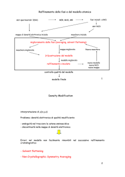
Ionization and dissociation processes can be summed up graphically as in Figure 1.1.
(
)↔
(
)
↔
(
)
↔
(
)
(
)
Figure 1.1: Description of solvation, ionization and dissociation processes on a standard solute compound A-B
) indicates the molecule still in the solid state, (
)
Where (
the solvated
)
compound - that is in liquid phase - (
the ion pair after ionization process and
( )
( )
the free ions in solution, after dissociation. The index solv indicates that
the species in parenthesis are within one solvent cage. Please note that each of these
transformations has a respective counter-reaction which, relatively to dissociation step, is
named association process.
These two phenomena (ionization and association/dissociation) are influenced in different
ways by solvents. Only solvents with sufficiently high permittivities will be capable of
reducing the strong electrostatic attraction between oppositely charged ions to such an extent
that ion pairs can dissociate into free solvated ions. Ion association is only noticeable in
aqueous solutions at very high concentrations because of the exceptionally high relative
permittivity of water, while they are found at much lower concentrations in alcohols, ketones,
carboxylic acids and ethers. In solvents of relative permittivities less than 10-15
(hydrocarbons, chloroform and acetic acid for example) practically no free ions are found; on
the other hand when the relative permittivity exceeds 40 (water and formic acid) ion
associates barely exist. In solvents of intermediate relative permittivity (ethanol or acetone for
instance) the ratio between free and associated ions depends on the structure of the solvent as
well as on the electrolyte [17].
Solubility Analysis and Modelling for Pharmaceutical Product Design
13
According to the common definition of thermodynamic phase as homogeneous region of
matter in terms of physical and chemical properties as well [3], both ionization and
dissociation processes can be seen strictly as phase transitions, since at least electrical
properties differ a lot from a simply solvated molecule, a ionized molecule and a dissociated
ion pairs. Somehow, then, in a solvent-solute system more than one phase transition could be
present and this should clarify again the complexity in describing the behavior of complex
systems involving both solid and liquid phases. Moreover, both ionization and
dissociation/association processes are really difficult to be mathematically characterized and
only few experimental data can be found in the open-literature, where mainly only qualitative
descriptions are available.
Regarding polyprotic compounds (which means that they are able to donate more than one
proton per molecule, such as carboxylic acids which are the solutes to make this enquiry on)
the ionization behavior can be somehow described with a series of pH-dependent equilibria
expressions. Here the behavior of Fumaric Acid is described as an example of the behavior of
a diprotic acid (such as Maleic, Succinic and Tartaric Acid too) while with a comparable
pathway it’s possible to characterize this phenomenon regarding a threeprotic acid as Citric
Acid. For completeness all behaviors are graphically in Appendix II while only the behavior
of Fumaric Acid is described here as an example. In relation to Fumaric Acid, then, two
subsequent dissociation equilibria must be considered as in Figure 1.2,
↔
↔
Figure 1.2: Dissociation equilibria of Fumaric Acid (H2A)
where and
are the equilibrium constants relative to the two dissociation steps.
Then, determination of the fraction of each of the three species involved requires both
equilibria to be taken into account. This leads to a set of three equations,
[
[
]
[
[
]
[
]
]([
[
]
,
(1.3)
,
(1.4)
]
]
,
[
]
)
(1.5)
where is the molar fraction of the species-i.
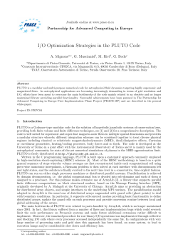
The speciation diagram of Figure 1.3 displays the pH distribution of the three species and it
has been obtained through equations (1.3), (1.4) and (1.5) where [H+] has been substituted
[ ].
with
14
Chapter 1
1,0
HA-
0,8
0,6
A2-
H2A
0,4
0,2
0,0
0
5
10
pH
Figure 1.3: Speciation diagram of ionization of Fumaric Acid as H 2A
Since
and
values of Fumaric Acid are close one to the other (the same is regarding
Fumaric and Succinic Acid) the mono-anion can exist only in a narrow pH range. This
HA- processes, but it
analysis can add something quantitatively to the understanding of dissolution
is still difficult to have a precise pH value of a complex solution while other phenomena such
as dissociation/association process should also be taken into account.
Summing up what has been described above, solubility is a very important property to take
into consideration in pharmaceutical drug production since it influences different steps of the
manufacturing process. Unfortunately there are no accurate models capable of precisely
describing all the aspects of solvation phenomena especially for complex systems as the ones
considered in this work.
Chapter 2
Thermodynamic background
In order to develop a mathematical solubility model, it is necessary first to perform a
thermodynamic enquiry on solubility description and dependences. Strictly, solubility can be
defined by the solid-liquid equilibrium description, but since the interactions between solute
and solvent are highly dependent on the compounds considered, these calculations can fit well
only to binary mixtures. Concerning ternary mixtures, first of all liquid-liquid equilibrium
calculations have to be considered in order to exclude from the investigation all those systems
characterized by a large miscibility gap, since the main interested is only in totally miscible
liquid systems. Solvent mixtures behavior could be then qualitatively described by excess
properties and combining this aspect together with solid-liquid equilibrium calculations, it
would possible to extend the description developed with regards to binary mixtures, also to
ternary systems.
2.1 Solid-Liquid Equilibria of Binary Mixtures
Phase equilibrium involving both solid and liquid states is the basis for describing solubility
behavior and its dependence on temperature, pressure and compounds considered. A rigorous
formulation of solid-liquid equilibrium - hence SLE - is here reported, while simplified
models, with regards to ideal and non-ideal behavior respectively are shown in the following
paragraphs. The basis for representing SLE is the iso-fugacity criterion [19]:
̂ ̂,
(2.1)
where uniformity of pressure and temperature is understood and ̂ is the fugacity of i-species
respectively in liquid (super-script L) and solid (super-script S) solution either.
With the introduction of the activity coefficients and with the assumption of ideal solution,
equation (2.1) becomes:
,
(2.2)
where and are the mole fractions of i-species in the liquid and solid systems respectively,
is the activity coefficient and is the fugacity of pure species, in each phase (see superscripts).
Equivalently:
,
(2.3)
18
Chapter 2
where:
⁄ .
(2.4)
The ratio of fugacities, at the temperature and pressure of the system, may be written in
expanded form:
(
)
(
)
(
(
)
)
⁄
(
⁄
)
(
⁄
)
(
)
⁄
(
)
,
(2.5)
where P and T are the system pressure and temperature, is the solid-liquid phase transition
temperature of pure species i and only one phase transition is expected.
Therefore the second ratio on the right side of equation (2.5) is unity because
at the
phase transition for pure species i. Hence:
(
(
(
)
)
⁄
)
⁄
(
.
)
(2.6)
Here, evaluation of requires expressions for the temperature effect on fugacity.
These expressions can be obtained through the definition of residual Gibbs energy as a
function of fugacity:
⁄ ,
where
Then:
(2.7)
is the residual Gibbs energy of i-species.
(
)
[
⁄
(
)
where is the residual enthalpy of i-species.
Integration of equation (2.8) for a single phase from
(
(
)
∫
)
⁄
]
,
(2.8)
to T leads to:
⁄
.
⁄
(2.9)
Equation (2.9) is applied separately to both solid and liquid phase. The resulting expressions
are substituted into equation (2.6), reduced by the following identity:
(
)
[(
) (
)]
,
(2.10)
where
is the enthalpy of the ideal gas referred to i-species.
This yields the rigorous expression:
∫
.
⁄
Evaluations of the integral proceeds as follows:
( )
( ⁄ )
∫
(2.11)
,
⁄
(2.12)
and
( )
Hence for each phase:
( )
(
⁄
)
(
(
⁄
)(
⁄
)
∫
⁄
)
⁄
(
∫
)
⁄
∫
.
⁄
(
(2.13)
)
. (2.14)
Solubility Analysis and Modelling for Pharmaceutical Product Design
19
Applying equation (2.14) separately to the solid and liquid phases and performing the
integration required by equation (2.11), yields:
∫
⁄
⁄
(
⁄
where
is the enthalpy change and
solid-liquid phase transition.
I is a complex integral defined by:
∫
[
(
⁄
⁄
)]
,
(2.15)
is the heat-capacity change, both regarding the
∫
⁄
)
∫
⁄
⁄
[
(
)
]
.
(2.16)
The system between equations (2.3), (2.11), (2.15) and (2.16) is what rigorously describes the
solid-liquid equilibrium of a mixture. Anyhow the full rigor of equation (2.15) especially is
rarely maintained and many simplified models have been developed in order to describe in an
easier way the behavior of these systems.
2.1.1 Ideal Behavior Model for Binary Systems
For several purposes equation (2.15) thoroughness is not needed and it is commonly
rearranged in a simpler way. In addition, the triple integral represented by I is a second-order
contribution and it is normally neglected. The phase transition between the solid and the
liquid phase can be identified with the only melting process, neglecting any other phenomena
involved in solvation, as described in §1.3.2. With these assumptions, equations (2.11) and
(2.15) together yield:
{
(
)
[
(
)]},
(2.17)
where
is the enthalpy change of melting, also known as heat of fusion,
is the
heat-capacity change of melting and
is the melting temperature, also known as freezing
point. It is necessary to underline that the heat-capacity change of melting is rarely available
and moreover the inclusion of the term involving
adds little to a qualitative
understanding of SLE.
With this assumption, equation (2.17) can be simplified in:
[
(
)].
(2.18)
In this work, also equation (2.3) could be rearranged. The solid-phase is constituted by a pure
component since none of the solvents under investigation would change from liquid to solid
phase in the temperature and pressure range considered. Then, for a pure compound
and
, yielding, with respect only to the solute:
.
(2.19)
The system of equations (2.17) and (2.19) is then the SLE thermodynamic model when ideal
behavior is expected.
20
Chapter 2
2.1.2 Models for Non-Ideal Behavior for Binary Systems
Even though the thermodynamic model proposed in §2.2.1 often provides decent results, the
complexity of the systems under investigation (a carboxylic acid with one or more organic
solvents) suggests to look upon more complex models, taking into account non-ideal
behaviors. Anyhow some assumptions of ideal behavior description are maintained, as the
complete immiscibility of solid phase - equation (2.19) - and neglecting the triple integral
contribution as well.
Unlike ideal SLE description, both terms involving heat-capacity and enthalpy changes of
solid-liquid phase transitions are not anymore identified by the only melting properties,
leading to a new equation for the fugacity ratio as follows [6] [14]:
(
)
∑
(
)
[
(
)]
, (2.20)
∑
[
(
)]
{
}
where solid-liquid phase transitions different from melting are considered separately as the
sum of contributes like
(
) and
[
(
)] where
is the
enthalpy change related to any single phase transitions j of i-species,
is the respective
heat-capacity change and
the temperature.
Unfortunately, as described in §1.3, it is very difficult to dispose of experimental data about
this kind of phenomena, so the accuracy of equation (2.20) is abandoned in favour of the
following simplified equation:
(
)
(
)
.
(2.21)
[
(
)]
{
}
In equation (2.21) the contribution of solid-phase liquid transitions is now described not only
through the melting term but also through an “apparent” term, taking into account all other
phenomena occurring during solvation process. Since data about the heat-capacity change of
melting are rarely available, it’s been decided to combine the melting term and all the others
referred to different phase-transitions in one only contribute, marked as “apparent”:
.
These assumptions lead to the introduction in the thermodynamic model of properties without
a real physical meaning, eliminating the possibility of a fully predictive model. It is evident
that experimental data are necessary in order to quantify the “apparent” properties.
Solubility Analysis and Modelling for Pharmaceutical Product Design
21
2.2 Liquid-Liquid Equilibria of Binary Mixtures
When different liquid compounds are mixed together to form a solution, they are not
necessarily miscible each other in all ratio and temperature ranges.
When a miscibility gap is present, then the mixture splits up in two or more different liquid
phases, each one characterized by a precise composition defined by thermodynamics.
For pharmaceutical purposes, it is highly recommended not to employ solvent mixtures
showing this behavior, in order to avoid the solute to distribute unequally in both liquid
phases with many complications for the following operations, described in §1.1. A liquidliquid phase stability investigation is needed as a preliminary calculation, in order to exclude
from ternary mixtures calculations all those systems containing two solvents showing
miscibility issues.
The thermodynamic criterion to determine the stability for a single phase binary mixture
employs the Gibbs energy change of mixing as the controlling property. More precisely, at
constant temperature and pressure the Gibbs energy change of mixing,
, and its first
and second derivatives must be continuous functions of the molar fraction of both compounds
and the second derivative must everywhere positive [19].
Thus:
.
The definition of the excess Gibbs energy,
(2.22)
:
∑
,
(2.23)
can be then rearranged, for a binary mixture, in:
.
(2.24)
Equation (2.24) can be used as a stability criterion, while equivalent expressions can be
developed by derivations, such as:
,
(2.25)
.
(2.26)
or passing through the Gibbs-Duhem equation:
All equations from (2.24) to (2.26) are equivalent expressions to determine the stability of a
single phase binary mixture: if they are satisfied, the liquid-liquid equilibrium is guaranteed.
If miscibility issues are detected through equation (2.24), (2.25) or (2.26), it is important to
quantify the immiscibility region, in order to exclude from calculations only those solvent
mixtures showing a large miscibility gap. Liquid-liquid equilibrium - hence LLE calculations are then needed.
The equilibrium model starts one more time from the iso-fugacity criterion:
̂
̂
.
(2.27)
22
Chapter 2
Where super-scripts α and β refer to the different liquid phases. Equation (2.27), with the
introduction of activity coefficients becomes:
.
(2.28)
If each pure species can exist as liquid at the temperature of the system:
,
whence:
.
(2.29)
Equation (2.29) provides a general and rigorous description of LLE for a multi-component
system. For a binary mixture, equation (2.29) results in:
,
(2.30a)
(
)
(
) .
(2.30b)
Equations (2.30a) and (2.30b) are usually rearranged in:
( )
( ),
( )
(
(2.31a)
).
(2.31b)
Since
, rather than , is a more natural thermodynamic function. Through equations
(2.31a) and (2.31b), then, the two liquid phase compositions can be calculated for each
solvent mixture, and all solutions showing a large miscibility gap can be excluded from
further evaluations.
Calculations have been performed in the temperature range between 0°C and 100°C and all
the results of this investigation are graphically shown in Appendix III, while here partially
miscible solvent mixtures are listed in following Table 2.1. It’s necessary to point out that this
simple enquiry has been carried out using equations (2.31a) and (2.31b) where activity
coefficients of two species in both phases have been calculated through the original UNIFAC
VLE model.
Table 2.1: List of partly miscible solvent mixtures with definition of lower
and upper non-miscibility limits at 25 C in terms of molar fraction of Water
Lower non-miscibility limit
Upper non-miscibility limit
Water – Methylethylketone
0.5619
0.9366
Water – Isopropylacetate
0.1262
0.9959
Water – Methyltertbutylether
0.3867
0.9966
Water – Tetrahydrofuran
0.2906
0.9892
Water – Ethylacetate
0.1659
0.9866
Water – Butylacetate
0.1031
0.9887
Water – Anisole
0.2508
0.9993
Solubility Analysis and Modelling for Pharmaceutical Product Design
23
It was expected that all solvent mixtures characterized by a large miscibility gap involve
water, because of the particular nature of water as a polar unsymmetrical compound. Other
mixtures have been found to show a small miscibility gap (Water - Isopropanol and Water Propanol) but the small extension of the non-miscibility area and the information found in
literature reveal that these predictions could be wrong, due to the thermodynamic model used
for activity coefficient calculation. That is why these mixtures have been considered as fully
miscible systems.
2.3 Analysis of Excess Properties of Binary Mixtures
Even though the largest part of solvent mixtures does not show a miscibility gap, this does not
mean that the behavior of the solution is ideal. Anyhow, a qualitative description of the
behavior of solvent mixtures is necessary in order to perform a solubility calculation of
ternary systems. The signs and relative magnitudes of the principal excess properties - Gibbs
energy, enthalpy and entropy, GE, HE and SE respectively - are useful for elucidating the
molecular phenomena which are the basis for the observed solution behavior.
Abbot at al. [20] have organized excess properties data for about 400 binary liquid mixtures in
a visual scheme which permits identification of patterns, trends and norms of behavior with
respect to mixture type. Excess properties for liquid mixtures depend primarily on
temperature and composition; therefore comparison of data for different mixtures is best done
at fixed T and x. Since many excess properties data are available at near-ambient
temperatures, T is chosen as 298.15 K and because extreme values for these properties often
occur near equimolar composition,
is fixed. The relation between the excess
properties into dimensionless form is:
.
GE/RT
III
Entropy Dominates
IV
Enthalpy Dominates
SE/R=0
(2.32)
Region 2
GE/RT
Region 4
SE/R=0
II
I
Enthalpy Dominates
Region 1
Region 0
IV
HE/RT
Entropy Dominates
V
Figure 2.1: Diagram of excess properties in skeleton
form as by Abbott et al.
HE/RT
Region 3
Region 5
Figure 2.2: Diagram of excess properties with 105
solvent mixtures under enquiry; new region definition
24
Chapter 2
Abbott et al [20] delineate a scheme where each combination of sign for the three excess
properties defines a region on the diagram in Figure 2.1, identified by domination of one of
these properties. Actually the purpose of excess properties analysis in this work leads to
define different regions, taking into account the magnitude of these quantities, instead of
signs. In fact, the main interest here is to define the distance of each solvent mixture from the
ideal behavior. It is important to underline that the region definition proposed here is
connected to the purpose of a qualitative description of solvent mixtures behavior. Results are
shown graphically in Figure 2.2.
It is interesting to notice that through this new definition, Regions 2 and 4 contain all solvent
mixtures showing large miscibility gap - as in Table 2.1 - together with other solvent mixtures
(Water-Isopropanol, Water-Ethanol and Water-Acetone) which shows anyhow a behavior far
from the ideal one - Water-Isopropanol shows really small miscibility gaps in liquid phase,
while Water-Ethanol and Water-Acetone shows a non-ideal behavior concerning the vaporliquid equilibrium. An unexpected behavior is shown by the following solvent mixtures:
Dimethylsulphoxide-Water, Dimethylsulphoxide-Methanol, Dimethylsulphoxide-Ethanol,
Dimethylsulphoxide-Propanol and Dimethylsulphoxide-Isopropanol - Region 5 and partly in
Region 3 - which, even though characterized by non-negligible values of excess properties,
are not predicted to split in liquid phases. This could be linked to the presence in these
systems of eutectic points or chemical reactions, not been pointed out by the previous liquidliquid equilibrium enquiry. Because of this, it is highly recommended to perform further
accurate investigations on these solvent mixtures, in order to define the behavior to be
expected. For this project purposes, then, these binary systems are held as they were partially
miscible solutions and excluded from ternary mixtures calculations. Considering all the other
mixtures, many of them are in Region 0 since they show very low contributions for all the
excess properties. This suggests that the respective solution behaviors could be considered as
ideal, while on the other hand, all mixtures showing not-negligible values for at least one of
the excess properties - Regions 1 and 3 - are considered non-ideal. The extrapolations of these
calculations on ternary mixtures solubility investigation are described in following §2.5, while
for completeness, the list of all solvent mixtures considered in this work with the qualitative
description of their behavior and their region in the excess properties diagram of Figure 2.2 is
shown in Appendix IV.
2.4 Extrapolation of Solid-Liquid Equilibria for Ternary Mixtures
As previously described, the solid-liquid equilibrium equation developed in §2.1 cannot be
used for a ternary mixture investigation. This is due to the fact that most of the phase
Solubility Analysis and Modelling for Pharmaceutical Product Design
25
transitions involved in these solvation processes are solvent-dependent, but in the model equation (2.15) - there are no indications for managing these phenomena in a solvent mixture.
The ternary mixture behavior is supposed to be linked to binary behaviors and excess
properties of the solvent mixture, but an explicit dependence especially from excess
properties is not explicit in thermodynamic formulation of SLE. The idea, then, is to
extrapolate what can be calculated in terms of solubility of solute in a single solvent with
regards to ternary mixtures considering excess properties only from a qualitative point of
view. Following what was analyzed in §2.4, here a model for solvent mixture ideal behavior
is proposed, while at the same time some suggestions concerning solvent mixtures showing a
non-ideal behavior are given.
2.5.1 Model of Ternary Systems for Ideal Solvent Mixtures
When an ideal behavior is predicted for a solvent mixture - that is when solvent mixture
considered appears in Region 0 of Figure 2.2 - then the solubility of the ternary system can be
calculated from the binary interactions. There are two ways to perform an ideal correlation of
binary data in order to extrapolate a model to describe the behavior of a ternary mixture. One
deals with a correlation of fugacity ratios, while the other deals with a correlation of the
properties present in the fugacity ratio description - equation (2.15).
The first method (named as “Model-1”) starts with the definition of
and
as the ratios
of fugacity of i-species - solute - with respect to solvent-1 and solvent-2 where it is important
to underline that here it is not important anymore which model has been used to describe the
mixture between the solute and each solvent: equations (2.17), (2.18) or (2.20). The
assumption of ideal solvent mixture leads to the statement that the interactions between the
two solvents (to be considered together with those between solute and each solvent) are
linear. Through the definition of solvent ratio, SR, as follows:
,
(2.33)
where xS1 and xS2 are the molar fractions in solutions of Solvent-1 and Solvent-2 respectively,
the ternary ratio of fugacities can be described as:
(
),
(2.34)
where
is the ternary system ratio of fugacities.
Equation (2.34) gives a way to evaluate the ratio of fugacities in a ternary mixture, while to
calculate the solubility it is necessary to merge it with equation (2.19).
The second method (“Model-2”) starts from the idea that equation (2.15) has been developed
not only in relation to binary mixtures, but theoretically for any mixtures. It has been chosen
to consider it only regarding binary systems because of difficulties in calculating some
properties when two solvents are present and all solvation phenomena become more
complicated. Anyway the purpose of this method is to make a linear correlation based on
26
Chapter 2
solvent ratio as in equation (2.34) but rather than on fugacity ratio, on the properties which
describe it. Considering the description of fugacity ratio as in equation (2.21) the ternary
apparent properties (
,
and
) can be calculated as in equation
(2.35):
(
),
(2.35)
where
and
are the binary values of apparent properties related to solvent-1
and solvent-2 respectively, SR is defined as in (2.34) and is the value of the apparent property
in the ternary mixture.
The accuracy of both models will be discussed in Chapter 4. Moreover, it’s important to
underline that the assumption of complete immiscibility in the solid phase can be considered
and that the system of equations to be used should be: (2.34) together with (2.19), or (2.21)
together with (2.19) where solvent-dependent properties have to be calculated as in equation
(2.35).
2.5.2 Models of Ternary Systems for Non-Ideal Solvent Mixtures
Where the solvent mixture considered in the ternary system investigation is expected to be far
from ideality, a linear correlation as shown in §2.5.1 cannot be used anymore. That is because
the magnitude of excess properties is not negligible and their contributions have to be
considered. Unfortunately it is not easy to make a mathematical estimation of the contribution
of excess properties of the solvent mixture to the ternary solubility model. Moreover, excess
properties have been calculated in particular conditions - fixed temperature and composition while their magnitudes could assume very different values and sometimes also change their
signs when calculated in different conditions. These remarks suggest leaving the idea of
developing a rigorous thermodynamic model for ternary mixtures investigation, while
different mathematic models can be recommended, each needing a certain number of
measurements in order to be able to fit well experimental-data. Even though this chapter
focuses on a thermodynamic overview of the problem, a brief description of the mathematical
model to be used will follow, while the complete explanation will take place in chapter 4.
The easiest way to correlate binary ratios of fugacities in a non-linear way is the simple
addition of one parameter. The way this parameter could be implemented in the equation for
the ternary ratio of fugacities highly depends on the shape of experimental-data. Here two
different dependences are shown (“Model-3” and “Model-4”, respectively) while in Chapter 4
it will be clarified how to choose the best one based on the experimental-data available:
(
)
(
),
(2.36)
(
) ( ) ,
(2.37)
where binary fugacity ratios,
, and solvent ratio,
, are defined as in §2.5.1, while k is
the parameter added to equation (2.34) in order to have a non-linear correlation. It is
Solubility Analysis and Modelling for Pharmaceutical Product Design
27
important to notice that equation (2.37) can be reduced to equation (2.34) when and it is
always able to keep extreme values (that is when solvent ratio is equal to 0 or 1) of ternary
ratio of fugacities equal to the binary. On the contrary, equation (2.36) cannot be reduced to
(2.34) with any values of the parameter k and it could be used only for solvent ratio values
between 0 and 1, extremes excluded.
Another opportunity to correlate binary fugacity ratios in order to extrapolate ternary fugacity
ratios deals with the definition of fugacity ratio obtained with the assumption of complete
immiscibility in the solid phase - equation (2.19). As a matter of fact to calculate this property
from experimental-data - that is, composition of the liquid phase and temperature - the
approach described by equation (2.19) is needed and it could be possible to match the linear
correlation of ternary fugacity ratio - equation (2.34) - through the definition of a new set of
UNIFAC binary-interaction parameters or through a slight modification of the temperature
dependence of these parameters. The main advantage of this method (which will be
mathematically described in chapter 4 by “Model-5”, “Model-6” and “Model-7”) is that the
same UNIFAC parameters set could be assumed to be able to describe well all the behaviors
of ternary mixtures involving the UNIFAC groups considered with the UNIFAC binaryinteraction parameters fine tuning. On the other hand, this approach is handling more than one
parameter, making the availability of more than one experimental-data compulsory.
Anyhow, a complete description of these models for ternary mixture solubility calculation is
shown in the following chapter 4.
Chapter 3
Solubility Modeling of Binary Mixtures
In chapter 2, four thermodynamic models - equations (2.17), (2.18), (2.20) and (2.21) characterized by a growing accuracy, have been proposed in order to calculate the solubility
relative to a binary mixture. All these models, describing the ratio of fugacities, can be linked
to the solubility through equation (2.19). In this chapter an analysis between the models
proposed is given and a detailed explanation of the procedure followed to reach the problem
solution is also presented.
3.1 Definition of a Mathematical Model for Binary Mixtures
It is now necessary to choose a mathematical model able to describe the behavior of the
systems under investigation between the models proposed in the previous chapter. The ideal
model of equation (2.18) is of course the simplest between those proposed but it does not
show any dependences of fugacity ratio on the solvent involved in the binary equilibrium. In
fact, equation (2.18) shows temperature dependence, but all properties involved are melting
properties relative to the pure solute. This means that, following the model described by
equation (2.18) - the fugacity ratio - that is at the same time the product between the molar
fraction of solute in liquid phase and its activity coefficient in solution, equation (2.19) - is
constant at fixed temperature, whatever solvent is involved in the binary mixture.
Experimental data disagree with the predictions of this model proving that it is too simple to
describe the behavior of APIs-solvents systems.
The model of equation (2.17) has the same problem since, even if it considers also the
contribution of the heat-capacity change of melting, it shows only dependences on the system
temperature and all properties involved are relative to the pure solute. In addition,
experimental-data relative to heat-capacity change of melting for the solutes considered in this
project are very rare. These considerations lead to reject also this model for the purposes of
this work. As expected, ideal models are lacking in accuracy and thermodynamic models for
non-ideal behaviors have to be considered even though they show other kinds of problems.
The fully rigorous model of equation (2.20) shows a dependence on the solvent involved in
the equilibrium through the addition of the contributions of other phase transitions than
melting. As physically explained in §1.3, these phenomena are strictly dependent on the
nature of the solvent considered and on the intermolecular forces involved. Anyway no data
30
Chapter 3
for enthalpy and heat-capacity changes of melting related to this kind of phenomena for the
systems under enquiry could be found in open-literature. Therefore, even though the model of
equation (2.20) is considered very accurate and promising, it is necessary to abandon the rigor
of this model in favor of the slightly simplified model of equation (2.21). Also the model of
equation (2.21) shows a dependence on the solvent involved in the equilibrium, not anymore
through real properties, but through apparent contributions added in order to take into account
all phase transitions occurring. The unavailability of phase transition data can be overcome by
calculating the “apparent” properties based on experimental data, but on the other hand this
means that solubility measurements are now compulsory in order to estimate the apparent
properties. Following this way, then, the original idea of a totally predictive model is not
feasible anymore, and the task now is to develop a model requiring the minimum number of
measurements. In order to estimate the minimum number of data needed, it is necessary to
rearrange equation (2.21) in a simpler form - equation (3.1) - underlining all the temperature
dependences described:
(
)
(
)
.
[
{
(
)]
(2.21)
}
(
).
(3.1)
In equation (3.1), the
property - the ratio of fugacities - is now substituted with a property
that could be thermodynamically described in the same way, but it is more common in the
pharmaceutical area: the solubility product,
. Equation (3.1) can be rearranged in order to
distinguish between those properties which could be found in literature - that is melting
properties - and those other properties which could be substituted simply by a parameter since
even though they have a precise physical meaning, they can’t be calculated.
(
).
(3.2)
Considering melting properties too as parameters but keeping them separated from the others
since they could be easily calculated, equation (3.2) becomes:
(
).
(3.3)
Where A and B, parameters which have to be calculated on properties available, are:
,
(3.4)
.
(3.5)
Solubility Analysis and Modelling for Pharmaceutical Product Design
31
While C, D and E parameters, which could be calculated only through a regression based on
experimental-data, are:
,
,
(3.6)
(3.7)
.
(3.8)
Since the purpose of this project is not the calculation of phase transition properties but rather
the development of a mathematical model able to calculate the solubility of a solute in binary
and ternary mixtures, the focus is on the model itself rather than on the properties.
Therefore the number of parameters to be calculated through a regression based on
experimental data is three - C, D and E - which means that three is the minimum number of
solubility measurement necessary in order to be able to give a value to all parameters.
Clearly, a larger regression based on more than three measurements would be more
representative. The whole solubility model here developed in relation to a binary system,
then, joining together equation (3.3) and (2.19), is:
(
).
(3.9)
Where the left term of the equation is able to calculate the solubility of the species i for any
temperature chosen - when parameter values are available - since it is function of the only
molar fraction of the solute when the solvent involved in the system is fixed.
3.2 Calculation Procedure
Once the mathematic model has been chosen - equation (3.9) - it is important to define the
calculation pathway needed. As mentioned above, for a binary system three solubility
measurements are strictly necessary to determine a complete parameter set. At the same time
it is evident that a parameter regression performed on more than three data should lead to a
better parameter set in terms of matching capability. The mathematic model represented by
equation (3.9) showed an unexpected numerical instability and in order to obtain a converged
optimization result, it was necessary to start with “good” values of parameters as initial
estimates. Since these parameters have been introduced just because there are no estimations
available in literature for the properties hidden inside these factors, a way to perform a
preliminary assessment is needed. An opportunity is to perform a first parameter optimization
based on only three experimental data. This would lead to a perfect match between
predictions and experimental measurements. At the same time a first estimation of the
parameter set would be available. With these initial estimates, a complete regression can be
performed - where more than three experimental data are regressed. The optimum parameter
32
Chapter 3
set corresponds to the set which minimize the objective function set, designed as the sum of
the relative errors:
√(
) .
(3.10)
Where and is calculated through equation (3.9). Results are reported in chapter 5, but it is
interesting to underline here that the parameter set calculated with only three experimental
data is rarely much different from the one obtained when the complete regression is
performed. This consideration leads to the conclusion that three measurements are not only
the minimum number needed for a complete set of parameters for the model, but they also
seem able to assure a good predictive capacity for solubility within the range of temperatures
investigated. For this reason it is strongly recommended, at the design of experiments stage,
to perform the three measurements in the largest temperature range possible. This means one
measurement around 0°C, a second measurement around 100°C and the third measurement at
a mean temperature, around 50°C, in order to take into account the whole temperature range
defined in the stated objectives.
Another aspect about the parameter regression is that the model of equation (3.9) is really
sensitive, meaning that a slight difference of parameter values reflects in a large change of the
prediction made. This is good to know since it is common to find in the literature slightly
different experimental solubility data referred to the same binary system in the same
conditions of temperature and pressure. If these differences are lower or around 5%, the
parameter set calculated on the first experimental data is still able to perform a good fit related
to new values.
Going deeply into the parameter optimization procedure, here is a step-by-step description of
the method adopted for this project and leading to results listed in Chapter 5, considering the
availability of only three data-points.
 Once experimental data - consisting in three couples of (
) values, where j
refers to the different measurement - are available, it’s necessary to calculate a value
for relative experimental solubility product
:
,
(3.11)

where
is calculated through original UNIFAC VLE model, with experimental
system composition and temperature.
Calculated solubility product, on the other hand, has to follow the model proposed in
equation (3.9):
(

),
(3.12)
which is actually possible to calculate for any of the three j-temperatures measured.
Ideal solubility products can be easily calculated through pure properties of the solute:
(
),
where A and B values has to be calculated as in equations (3.4) and (3.5).
(3.13)
Solubility Analysis and Modelling for Pharmaceutical Product Design

Then the non-ideal contribute can be calculated as ratio:
.

(3.14)
Imposing for every j-measurement that leads to a system of three algebraic equations:
(
)(
(
(
(
(
Where
33
(
)
)
,
)
)
(3.15)
)
,
(3.16)
.
(3.17)
) and sub-scripts refer to the three j-measurements.
This procedure leads to a complete set of parameter able to perfectly match the three
experimental solubility data available. When more than three measurements are accessible,
then a complete optimization has to be done. Initial estimates for parameter values are those
calculated through equations (3.4), (3.5), (3.15), (3.16) and (3.17), while objective function to
be minimized is simply the sum of relative errors:
∑(
) .
(3.18)
It could be useful to evaluate the goodness of fitting also through the statistical index R2,
known as coefficient of determination either, defined as follows:
,
(3.19)
where SSE and SST, sums of squares of errors and totals respectively are defined as:
∑(
) ,
(3.20)
∑(
̅) ,
(3.21)
where
is the observed - here experimental - value,
the associated modelled - here
calculated - value and ̅ the mean of observed data respectively.
The model defined in §3.1, adopted as in §3.2, has been tested on 13 different binary mixtures
and the results of the fitting are shown in numerical and graphical forms in chapter 5.
Chapter 4
Solubility Modeling of Ternary Mixtures
The more challenging side of the development of a model representing solubility of complex
systems is the solubility prediction of ternary mixtures. Here all models briefly defined in
§2.5 are accurately described from a mathematical point of view, then the step-by-step
procedure followed in order to obtain the results presented in chapter 5 is given.
4.1 Definition and Description of Mathematical Models for Ternary
Mixtures
As described in §2.5 the behavior of a ternary mixture in terms of solubility is assumed to be
connected both to binary mixtures behaviors, of the solute with each of the two solvents
involved in the ternary mixture, and to excess properties characterizing the solvent mixture.
Unfortunately the thermodynamic model describing solid-liquid equilibrium in a mixture
which could be multicomponent does not show any explicit dependences of solubility on
binary characterization or on excess properties of the mixture. That is why, in order to
overcome this problem, different extrapolation models have been proposed, in order to be
able to describe well the phenomena occurring in a ternary mixture, always considering the
necessity of performing the minimum number of experimental measurements.
Different models adopted will be described here one by one, always keeping in memory that
the binary model to refer to is the one described in the previous chapter by equation (3.9).
4.1.1 Linear Correlation of Solubility Product Parameters
The first and easiest way to extrapolate the solubility behavior of a ternary mixture is to make
a linear correlation of the two binary models between the solute and each solvent. What
described thermodynamically through equation (2.34) - which is “Model-1” - when translated
to the mathematical model leads to:
(
),
(4.1)
where solvent ratio SR is defined as in equation (2.33) and the two binary solubility products
referred to each solvent are calculated as in equation (3.9).
The big advantage of this simple model is that it has no parameters and so the ternary
solubility product can be calculated only through binary solubility products and solvent ratio.
36
Chapter 4
On the other hand, this model can be suitable, just because of its simplicity, only to a few
ternary mixtures, when the behavior expected is really close to the ideal. It is assumed that
most of the solvent mixtures included in Region 0 of Figure 2.2 - listed in Appendix IV show such an ideal behavior and then all ternary systems involving a solvent mixtures
characterized by very low values of both excess enthalpy and Gibbs energy should be fitted
pretty well even by this simplified model.
Unfortunately there are no data available referring to such a ternary system, then the
assumption made here cannot be proved by now.
4.1.2 Linear Correlation of Solubility Product Parameters
Another simplified model - “Model-2” - which adds only a minor accuracy to the one
described in §4.1.1 uses again a linear correlation, but this time it is not performed anymore
on binary solubility product values, but on solubility product parameters of equation (3.9).
Equation (2.35) argued that all “apparent” properties - which are actually solvent dependent of ternary mixtures could be extrapolated through a linear correlation form those relative to
each binary mixture. Actually, when considering equation (3.9) to characterize the ternary
mixture behavior, there is not an explicit dependence of solubility product on apparent
properties. Then the linear correlation should be performed on the solubility product
parameters themselves, in order to pursue the same aim.
To be more precise, ternary solubility model parameters should be calculated as follows:
(
).
(4.2)
Where M is each parameter taking part to the non-ideal part of the solubility product - that is
C, D and E. Actually A and B are not influenced by the solvent involved in the mixture, since
they are calculated only from pure solute properties - equations (3.4) and (3.5) - and then
performing a correlation on their values too, even though leading to a mathematical
equivalent result, since A and B have the same numerical values with any solvent considered,
would have no meanings from a thermodynamic point of view.
This model has the same big advantage of the one described in the previous paragraph, since
the absence of adding parameters reflects on a predictive ability of the ternary solubility only
having binary parameters available. On the other hand, this model is very simplified and, even
though it adds little accuracy to the ideal model of §4.1.1, it could not be extended to any
ternary systems. It should be suitable for almost all systems showing two solvents defined in
Region 0 of Figure 2.2 and also for some systems showing two solvents in the closer part of
Regions 1, 2 and 3, where excess properties still have low values. Moreover the unavailability
of experimental data referring to such a system let assumptions made here with no
demonstrations.
Solubility Analysis and Modelling for Pharmaceutical Product Design
37
4.1.3 Parametric Models
Leaving the category of ideal model, the simplest way to define a non-ideal model is through
the addition of one parameter. As described in the thermodynamic characterization of §2.5.2,
there are at least two different ways - equations (2.36) and (2.37) - to add a parameter to the
simple ideal model and they differ pretty much one from the other. The decision to consider
one parametric model instead of the other one is based simply on the shape that experimental
solubility products show plotted against the solvent ratio.
The model described by equation (2.36) and named “Model-3”, can be mathematical
rearranged as follows:
(
)
(
),
(4.3)
Where the parameter added - k in equation (2.36) - is here named F.
This model leads again to a linear trend of ternary solubility product as a function of solvent
ratio, but this time it is shifted to higher or lower values, depending on the value of the
parameter. Compared to the model presented in §4.1.1 and §4.1.2 - “Model-1” and “Model-2”
- the main advantage of “Model-3” is that the presence of only one parameter more makes the
model suitable to almost any kind of ternary mixture since varying the value of that
parameter, it would be possible to match experimental data even far from the ideal linear
correlation - equation (4.1). On the other hand, there are also some disadvantages. First of all
the introduction of one parameter reflects into the need of at least one ternary experimental
data in order to fit it, then the biggest disadvantage of this model is that even though it should
be able to fit well different experimental-data, the value of the parameter is highly
temperature-dependent, meaning that once an optimization has been done based on one only
solubility measurement, the model developed is predictive only at the temperature of that
measurement and no others. This means that actually one measurement is needed for every
temperature at which it is interesting to have a solubility calculation.
Similarly, the second parametric model proposed in §2.5.2 - “Model-4” of equation (2.37) can be described through the mathematical model as follows:
(
) ( ) ,
(4.4)
Where the parameter added is named G in order to avoid any misunderstandings with other
parameters defined.
The main difference between this parametric model and the one described by equation (4.3) is
that “Model-4” follows a power law. Of course, since the solvent ratio can assume values
between 0 and 1, the trend of ternary solubility product against solvent ratio would never be
extremely far from the linear one, but it could easily fit to experimental data showing a nonlinear trend against the solvent ratio. The main advantages and disadvantages of this method
are the same which concern the first parametric model. It is interesting to observe that this
model degenerates into the linear model when and it is also able to describe extreme ternary
38
Chapter 4
solubility products - which are binary, actually - while the model described by equation (4.3)
could not. It is necessary to underline, furthermore, that even if only one experimental-data
could be enough to decide to perform ternary solubility calculation through a parametric
model instead of the linear model of equation (4.1), more than one measurement is needed in
order to choose between these two parametric models. The main difference is relative to the
expected trend of ternary solubility product against solvent ratio - linear following “Model-3”,
a power law following “Model-4” - and the only way to discern between these two models is
having a perception on the trend of the experimental data and this is feasible only having
more data available.
4.1.4 Fine Tuning of UNIFAC Binary Interaction Parameters
In order to avoid performing one measurement for each temperature to be investigated, one
could deal not anymore with the right side of equation (3.9), but try to fit the left side to the
linear prediction of equation (4.1) - “Model-1”.
(
).
(3.9)
The left side of equation (3.9), actually, consists of the molar fraction of the solute and of the
relative activity coefficients, depending on temperature and species involved in the
equilibrium - besides on the molar fraction itself. Since these are all characteristics of the
system under investigation - and they are fixed - the only way to deal with the left side of the
equation (3.9) is to change the value of activity coefficients, in order to be able to match the
linear Model-1 of equation (4.1) in order not to add any other parameter.
Analyzing the original UNIFAC VLE model [21] - which has been adopted, actually, for all
calculations concerning this project and it is described in Appendix V - it is possible to
perform a fine tuning only on the binary interaction parameters . These parameters, broadly,
indicates the interactions between two different groups when in the same system and this is
exactly what is needed in this investigation. Since most of the species are defined through
UNIFAC models by more than one group, it is necessary to choose the parameters to be tuned
among all parameters used to perform the equilibrium calculation.
The principle adopted here is to choose the most peculiar group for every species, more
precisely the functional group when present. Then, for instance, for all alcohols the -OH
group will be taken into account and similarly for all solutes considered in this work - which
are carboxylic acids - the -COOH group will be considered. A complete list of the UNIFAC
groups to be taken with respect to every compound defined in this project is present in
Appendix VI. Clearly, only the binary interaction parameters between a solute-group and a
solvent-group for each solvent have to be fine tuned, while binary interaction parameters
between the two solvents have to be kept constant, in order not to change liquid-liquid
equilibria calculations. Therefore, since a ternary mixture involves two solvents and one
Solubility Analysis and Modelling for Pharmaceutical Product Design
39
solute, there are four parameters for every ternary system to be tuned. This reflects in the need
of at least four solubility measurements in order to perform the optimization. These
measurements should be done at different temperatures and solvent ratios, in order to wellcharacterize the largest range possible.
There are several advantages which make this model - “Model-5” - preferable than the others
described so far. First of all, it should be able to fit to any kind of ternary mixtures under
investigation, since ideal behaviors would be fitted by the original UNIFAC VLE parameters,
while all the others could be well matched through the optimization of four parameters which lead, actually, to a much better fitting than with only one parameter, indeed.
Secondarily, the same parameter set should be able to well describe the system behavior at
different temperatures, so that each set could be defined on the system to characterize and not
on a precise temperature too. Therefore, it can be assumed that a new parameter set obtained
through this method could be able to match not only experimental data relative to the ternary
system investigated, but also experimental data relative to other ternary systems slightly
different from that one. Trying to clarify this concept through an example, when the ternary
system between Fumaric Acid- Water-Isopropanol has been well fitted through a new
UNIFAC binary interaction parameter set, then all other ternary mixtures acid-water-alcohol
should be well described. This is because with the first optimization, binary interaction
parameters between -COOH group and H2O and -OH groups respectively have been tuned
and it could be assumed that these parameter values can describe well all similar systems.
Unfortunately also this assumption cannot be proved since experimental-data relative to only
one ternary system - Fumaric Acid-Water-Isopropanol - are available. The disadvantage of
“Model-5” is that it needs at least 4 experimental-data in order to make the optimization and
moreover it is very difficult to perform a perfect match with these 4 measurement since an
algebraic solution - as in §3.2 - is not feasible and a numeric approach rarely leads to
satisfactory results, because of the high non-linearity of the system.
Another improvement to this advanced extrapolation model can be done. The original
UNIFAC VLE model does not show any temperature dependence of binary interaction
parameters, differently than other UNIFAC models. This can lead to a non-accurate model,
since group interactions are indeed temperature dependent. Therefore, temperature
dependence can be added to the description of UNIFAC binary interaction parameters. More
precisely, there are at least two different opportunities to implement a basic temperature
dependence of UNIFAC binary interaction parameters definition, as follows:
,
(4.5)
.
(4.6)
Where
is the new parameter added in order to lead to have temperature dependence.
Equations (4.5) and (4.6) describe “Model-6” and “Model-7” respectively. The number of
parameters to be tuned is now eight - four and four - so that eight measurements are needed.
40
Chapter 4
The improvement which could be obtained through this model consists in a more precise
temperature dependence of activity coefficients in order to be able to match easily ternary
solubilities relative to very different temperatures. Compared to the simple UNIFAC binary
parameters fine tuning of “Model-5”, the only disadvantage is the number of experimental
data needed. On the other side, however, the larger amount of parameters would lead to a
much better fitting and probably also to a more probable suitable of the same parameter set to
different systems - unless similar as regards to compounds involved.
4.2 Calculation Procedure
All the opportunities to extrapolate ternary mixture solubility behavior from the binary
interactions have been exhaustively described in §4.1 through seven different models. Here
the step-by-step procedure to be followed to perform all necessary calculations is shown,
similarly to what described §3.2. It is assumed that binary solubility products have to be
calculated through (3.9) using the procedure described in §3.2 and here different approaches
are shown, depending on the number of experimental-data available.
4.2.1 Zero ternary experimental-data pathway
When no experimental data are available, only models described through (4.1) and (4.2) are
suitable. In these cases the approach is simple since it consists of a few steps and some
assumptions:
 Calculate excess properties of solvent mixture as described in §2.4, at fixed
temperature and composition;
 Determine on diagram of Figure 2.2 the region where the solvent mixture is included;
 If the solvent mixture is described by really low values of excess properties and it is
part of Region 0 in the diagram of Figure 2.2, then the “Model-1” - equation (4.1) should be chosen;
 If the solvent mixture is described by pretty low values of excess properties and it is

part of Regions 1, 2 and 3 close to the axis-origin in the diagram of Figure 2.2, then
the “Model-2” - equation (4.2) - could be able to well predict the ternary system
behavior.
If the solvent mixture is described by medium or high values of excess properties and
it is part of Regions 1, 2 and 3 far from the axis-origin or Regions 4 and 5 either in the
diagram of Figure 2.2, then an ideal model is not able to accurately describe the
behavior of such systems and at least one measurement is needed.
Solubility Analysis and Modelling for Pharmaceutical Product Design
41
4.2.1 One ternary experimental-data pathway
When one experimental-data is available, also parametric model - “Model-3” of equation
(4.3) and “Model-4” of equation (4.4) - can be suitable in order to describe the ternary
mixture solubility behavior. Considering all binary calculations just performed, the procedure
to be followed is:
 Calculate the experimental solubility product relative to the only measurement
available, as in equation (3.10);
 Compare the experimental solubility product obtained with the calculated solubility
product at the same temperature and solvent ratio predicted by “Model-1” and
“Model-2” - equations (4.1) and (4.2) respectively;
 If one of the ideal models is able to fit well the experimental solubility product, then
that model could be chosen in order to describe the behavior of that system;
 If none of the ideal models is able to fit well the experimental solubility product, then
one of the parametric models - “Model-3” of equation (4.3) and “Model-4” of
equation (4.4) - could be chosen;
 The algebraic calculation in order to determine the value of F or G parameter consist
of one linear equation and of a power law equation respectively, but they all are
simple to be solved.
It is important to underline here that to set the parameter value calculated in relation to one
only data-point to describe the behavior of the same system also in relation to other different
temperature is such a hard assumption and it’s strongly not recommended. Moreover, to
discern between the two parametric models which could for sure lead to a perfect match
relative to one only data-point, it is necessary to have more than one solubility measurement
available.
4.2.3 More ternary experimental-data
When more than one experimental-data is available, also the “Model-5”, “Model-6” and
“Model-7” can be used.
The procedure to be followed now is more complicated, especially because it would strongly
depend on the precise number of experimental-data available - when less than 8 measurement
are available, for example, the full “Model-6” and “Model-7” cannot be used, while when less
than 4 data are available, neither “Model-5” can be suitable, actually. So, the pathway
presented here starts with the assumption that eight or more experimental-data are available,
so that all models could be used.
 Calculate all the experimental solubility products relative to each experimental
measurement as in equation (3.10);
42
Chapter 4






Compare the experimental solubility products obtained with the calculated solubility
products at the same temperatures and solvent ratios predicted through “Model-1” and
“Model-2” described by equations (4.1) and (4.2) respectively;
If one of the ideal models is able to fit well the experimental solubility products, then
that model could be chosen in order to describe the behavior of that system;
If none of the ideal models is able to fit well the experimental solubility products, then
one of the parametric models - “Model-3” of equation (4.3) and “Model-4” of
equation (4.4) - could be chosen;
The determination of optimum value of F or G parameter does not consist anymore in
a simple algebraic calculation and a complete regression is needed, even though every
different system temperature should lead to different parameter values so that
depending on the amount of measurement at the same temperature a simple algebraic
equation can solve the fitting problem - when only one data-point is available at a
certain temperature, then an algebraic equation would be the resolving system, while
more than one measurement would lead to a optimization process, using the objective
function described through equations (3.10) and (3.17).
If none of the parametric models is able to fit well the experimental solubility
products, then one of the UNIFAC-based models - “Model-5”, “Model-6” and
“Model-7” - could be chosen.
Depending mainly on the amount of measurements available one of the three UNIFAC
binary interaction parameters tuning models could be chosen, where it is important to
underline that “Model-6” and “Model-7”, even though pretty heavy from a
computational point of view, are supposed to be the most accurate model here
proposed and they are highly recommended. The optimization process follows the
same steps listed in §3.2, through equations (3.10) and (3.17).
All these models have been tested on the only available set of ternary experimental-data and
results in terms of comparison between experimental solubilities and modeled solubilities are
given in following chapter 5.
Chapter 5
Results and Discussion
All binary and ternary solubility models have been described from a physicochemical point of
view in chapter 2 and from a mathematical point of view in chapters 3 and 4 respectively.
Results are reported in this chapter. This chapter is divided into two main paragraphs, relative
to binary and ternary results respectively. Results are shown numerically - through the
exhibition of parameters values when needed by the models and of indexes useful to define
the goodness of the prediction - and graphically as well - through comparative charts. Every
paragraph is followed by a brief discussion of results, where some comments and
considerations are presented. It is important to underline that all regressions - excluding
simple algebraic calculations - have been performed through the setting of different programs
implemented using one of the ICAS [22] tools: MoT. Moreover an excel-based complete
program is under construction, in order to collect all the programs developed in a simple and
user-friendly interface.
5.1 Binary Mixtures Results
Concerning binary mixtures, experimental-data are available for 13 different binary systems:
those between all the five organic acids considered as solutes and Water and, in relation to
Fumaric and Succinic Acid, also with Acetone, Ethanol, Isopropanol and Propanol. Tabled
results are simple to understand and they include parameter values, mean error, maximum
error and the coefficient of determination R2 as indexes useful to evaluate the goodness of the
fitting. Charts show the comparison between experimental values, calculated values and also
ideal values in order to quantify the distance of each system from the ideal behavior. Charts
take into account only solubility values - intended as the saturation molar fraction of solute
dissolved - since the same charts relative to solubility products show similar results in terms
of mean and maximum errors, as displayed in relation to the first binary system considered:
Citric Acid-Water. For completeness, these charts are included in Appendix VII.
More precisely, solubility charts displays:
 Experimental Data, that is
in the y-axis versus
in the x-axis;
 Ideal Prediction, that is
in the y-axis versus T in the x-axis, where:
[
(
⁄ )]⁄ .
(5.1)
46
Chapter 5

Where A and B parameters are calculated as in equations (3.4) and (3.5) respectively
and
is calculated with Original UNIFAC VLE at relative temperature and
composition;
Calculated Data, that is
in the y-axis versus T in the x-axis, where:
[
(
⁄
⁄
)]⁄ .
(5.2)
Where A and B are calculates as in equations (3.4) and (3.5) respectively, while C, D
and E parameters are calculated through the complete optimization procedure
described in §3.2. is calculated with Original UNIFAC VLE at relative temperature
and composition.
In relation to solubility product charts - here present only in relation to the binary system
between Citric Acid and Water while all the others are in Appendix VII - instead, there are
displayed:
 Experimental Data, that is
in the y-axis - as in equation (3.11) – versus
in
the x-axis;
 Ideal Prediction, that is
in the y-axis - as in equation (3.13) – versus T in the xaxis;
 Calculated Data, that is
in the y-axis - as in equation (3.12) – versus T in the xaxis.
5.1.1 Citric Acid – Water
0,3
Solubility product
0,25
Experimental Data
Table 5.1: Binary parameters for
the system Citric Acid-Water
Ideal Prediction
Calculated Data
0,2
A
B
C
D
E
10.753
-4582.37
-52.385
4898.09
6.6514
0,15
Table 5.2: Indexes of the
goodness of fitting relative to
solubility product Calculated
Data for the system Citric AcidWater
0,1
0,05
0
283,15
328,15
373,15
Temperature [K]
Figure 5.1: Experimental data, ideal prediction and
calculated data of solubility product of the system
Citric Acid-Water
Mean Error
Maximum Error
R2
3.09%
6.36%
0.9977
Molar Fraction Solubility
Solubility Analysis and Modelling for Pharmaceutical Product Design
0,40
Experimental Data
0,35
Ideal Prediction
0,30
47
Calculated Data
Table 5.3: Indexes of the goodness of fitting relative to
solubility Calculated Data for the system Citric Acid-Water
0,25
0,20
Mean Error
Maximum Error
3.09%
6.36%
0,15
0,10
0,05
0,00
283,15
328,15
373,15
Temperature [K]
Figure 5.2: Experimental data, ideal prediction and calculated
data of solubility of the system Citric Acid-Water
Differences between solubility product and solubility charts are very low, then only the
solubility charts are shown. Those relative to solubility products are in Appendix VII.
Molar Fraction Solubility
5.1.2 Maleic Acid – Water
0,40
Experimental Data
0,35
Ideal Prediction
0,30
Table 5.4: Binary parameters for
the system Maleic Acid-Water
Calculated Data
A
B
C
D
E
7.6184
-3078.97
-36.467
3141.40
4.6814
0,25
0,20
0,15
Table 5.5: Indexes of the goodness of fitting relative to
solubility Calculated Data for the system Maleic AcidWater
0,10
0,05
0,00
273,15
313,15
353,15
Temperature [K]
Figure 5.2: Experimental data, ideal
prediction and calculated data of solubility
of the system Maleic Acid-Water
Mean Error
Maximum Error
1.26%
2.59%
48
Chapter 5
5.1.3 Tartaric Acid – Water
0,35
0,30
Experimental Data
Table 5.6: Binary parameters for
the system Tartaric Acid-Water
Ideal Prediction
Molar Fraction Solubility
Calculated Data
0,25
0,20
A
B
C
D
E
7.7307
-3418.14
-41.227
3695.13
5.2695
0,15
0,10
Table 5.7: Indexes of the goodness of fitting relative to
solubility Calculated Data for the system Tartaric
Acid-Water
0,05
0,00
273,15
323,15
373,15
Temperature [K]
Mean Error
Maximum Error
0.40%
1.47%
Figure 5.4: Experimental data, ideal
prediction and calculated data of solubility
of the system Tartaric Acid-Water
5.1.4 Succinic Acid – Water
0,12
Experimental Data
Ideal Prediction
Molar Fraction Solubility
0,10
Table 5.8: Binary parameters for
the system Succinic Acid-Water
Calculated Data
0,08
0,06
A
B
C
D
E
13.909
-6386.45
145.26
-3742.54
-22.555
0,04
0,02
0,00
273,15 293,15 313,15 333,15 353,15
Temperature [K]
Figure 5.5: Experimental data, ideal
prediction and calculated data of solubility
of the system Succinic Acid-Water
Table 5.9: Indexes of the goodness of fitting relative to
solubility Calculated Data for the system Succinic
Acid-Water
Mean Error
Maximum Error
3.11%
7.61%
Solubility Analysis and Modelling for Pharmaceutical Product Design
49
5.1.5 Succinic Acid – Acetone
0,035
0,03
Experimental Data
Table 5.10: Binary parameters for
the system Succinic Acid-Acetone
Ideal Prediction
Molar Fraction Solubility
Calculated Data
0,025
0,02
A
B
C
D
E
13.909
-6386.45
18.493
2746.69
-4.1892
0,015
0,01
Table 5.11: Indexes of the goodness of fitting relative
to solubility Calculated Data for the system Succinic
Acid-Acetone
0,005
0
282,85 292,85 302,85 312,85
Temperature [K]
Mean Error
Maximum Error
0.88%
1.89%
Figure 5.6: Experimental data, ideal
prediction and calculated data of solubility
of the system Succinic Acid-Acetone
5.1.6 Succinic Acid – Ethanol
0,14
0,12
Experimental Data
Table 5.12: Binary parameters for
the system Succinic Acid-Ethanol
Ideal Prediction
Molar Fraction Solubility
Calculated Data
0,1
0,08
A
B
C
D
E
13.909
-6386.45
-79.239
6696.79
10.744
0,06
0,04
Table 5.13: Indexes of the goodness of fitting relative
to solubility Calculated Data for the system Succinic
Acid-Ethanol
0,02
0
284,25
304,25
324,25
Temperature [K]
Figure 5.7: Experimental data, ideal
prediction and calculated data of solubility
of the system Succinic Acid-Ethanol
Mean Error
Maximum Error
3.06%
12.35%
50
Chapter 5
5.1.7 Succinic Acid – Isopropanol
Molar Fraction Solubility
0,1
Table 5.14: Binary parameters for
the system Succinic AcidIsopropanol
Experimental Data
0,09
Ideal Prediction
0,08
Calculated Data
0,07
A
B
C
D
E
0,06
13.909
-6386.45
83.132
-641.42
-13.448
0,05
0,04
0,03
Table 5.15: Indexes of the goodness of fitting relative
to solubility Calculated Data for the system Succinic
Acid-Isopropanol
0,02
0,01
0
282,75
302,75
322,75
Temperature [K]
Mean Error
Maximum Error
1.48%
3.71%
Figure 5.8: Experimental data, ideal
prediction and calculated data of solubility
of the system Succinic Acid-Isopropanol
Molar Fraction Solubility
5.1.8 Succinic Acid – Propanol
0,16
Experimental Data
0,14
Ideal Prediction
0,12
Table 5.16: Binary parameters for
the system Succinic Acid-Propanol
Calculated Data
0,1
A
B
C
D
E
13.909
-6386.45
-509.33
25480.31
75.120
0,08
0,06
Table 5.17: Indexes of the goodness of fitting relative
to solubility Calculated Data for the system Succinic
Acid-Propanol
0,04
0,02
0
283,55
303,55
323,55
Temperature [K]
Figure 5.9: Experimental data, ideal
prediction and calculated data of solubility
of the system Succinic Acid-Propanol
Mean Error
Maximum Error
2.41%
8.40%
Solubility Analysis and Modelling for Pharmaceutical Product Design
51
Molar Fraction Solubility
5.1.9 Fumaric Acid – Water
0,009
Experimental Data
0,008
Ideal Prediction
0,007
Calculated Data
0,006
Table 5.18: Binary parameters for
the system Fumaric Acid-Water
A
B
C
D
E
7.1500
-4005.06
-158.65
7695.85
23.343
0,005
0,004
Table 5.19: Indexes of the goodness of fitting relative
to solubility Calculated Data for the system Fumaric
Acid-Water
0,003
0,002
0,001
0,000
273,15
313,15
353,15
Mean Error
Maximum Error
0.53%
2.27%
Temperature [K]
Figure 5.10: Experimental data, ideal
prediction and calculated data of solubility
of the system Fumaric Acid-Water
5.1.10 Fumaric Acid – Acetone
0,014
Experimental Data
Ideal Prediction
0,012
Table 5.20: Binary parameters for
the system Fumaric Acid-Acetone
Molar Fraction Solubility
Calculated Data
0,01
0,008
A
B
C
D
E
7.1500
-4005.06
116.76
-3794.25
-18.039
0,006
0,004
Table 5.21: Indexes of the goodness of fitting relative
to solubility Calculated Data for the system Fumaric
Acid-Acetone
0,002
0
279
299
319
Temperature [K]
Figure 5.11: Experimental data, ideal
prediction and calculated data of solubility
of the system Fumaric Acid-Acetone
Mean Error
Maximum Error
0.51%
2.12%
52
Chapter 5
5.1.11 Fumaric Acid – Ethanol
Molar Fraction Solubility
0,05
Table 5.22: Binary parameters for
the system Fumaric Acid-Ethanol
Experimental Data
0,045
Ideal Prediction
0,04
Calculated Data
0,035
A
B
C
D
E
7.1500
-4005.06
-21.833
2931.19
2.5291
0,03
0,025
0,02
Table 5.23: Indexes of the goodness of fitting relative
to solubility Calculated Data for the system Fumaric
Acid-Ethanol
0,015
0,01
0,005
0
279
299
319
339
Mean Error
Maximum Error
1.58%
4.39%
Temperature [K]
Figure 5.11: Experimental data, ideal
prediction and calculated data of solubility
of the system Fumaric Acid-Ethanol
Molar Fraction Solubility
5.1.12 Fumaric Acid – Isopropanol
0,08
Experimental Data
0,07
Ideal Prediction
Table 5.24: Binary parameters for
the system Fumaric AcidIsopropanol
Calculated Data
0,06
0,05
A
B
C
D
E
7.1500
-4005.06
-12.008
2266.83
1.2342
0,04
0,03
0,02
Table 5.25: Indexes of the goodness of fitting relative
to solubility Calculated Data for the system Fumaric
Acid-Isopropanol
0,01
0
279
299
319
339
Temperature [K]
Figure 5.13: Experimental data, ideal
prediction and calculated data of solubility
of the system Fumaric Acid-Isopropanol
Mean Error
Maximum Error
2.83%
10.31%
Solubility Analysis and Modelling for Pharmaceutical Product Design
53
5.1.13 Fumaric Acid – Propanol
0,06
Experimental Data
Table 5.26: Binary parameters for
the system Fumaric Acid-Propanol
Ideal Correlation
Molar Fraction Solubility
0,05
Calculated Data
0,04
A
B
C
D
E
7.1500
-4005.06
-73.625
5159.70
10.286
0,03
0,02
Table 5.27: Indexes of the goodness of fitting relative
to solubility Calculated Data for the system Fumaric
Acid-Propanol
0,01
0
279
299
319
339
Temperature [K]
Mean Error
Maximum Error
2.45%
7.48%
Figure 5.14: Experimental data, ideal
prediction and calculated data of solubility
of the system Fumaric Acid-Propanol
5.2 Discussion of Binary Mixture Results
Results of solubility modeling concerning binary mixtures have to be discussed, actually,
from at least two very different points of view. The first is simply regarding the goodness of
fitting, while the second is dealing with parameter values, in order to be able to make some
considerations linking together what described in §1.3.2 and in §3.1. The fitting quality could
be evaluated through different indexes. In this project the relative error has been chosen
because of its intuitive meaning, while the coefficient of determination has been calculated
only regarding solubility product charts and they are tabled in Appendix VII.
Considering all binary mixture results, the mean error is never larger than 3%, and at the same
time the maximum error rarely - only twice where 125 measurements have been considered exceeds the target of 10%. Meanwhile, also values of coefficient of determination are
satisfactory since the minimum between thirteen binary systems considered is 0.9951
concerning the system between succinic acid and ethanol, where the largest relative error has
been found. Considering these results and at the same time considering graphical results
presented in §5.1 and in Appendix VII, it can be stated that the fitting performances are
satisfactory and the model here developed is able to describe well the behavior of the thirteen
binary systems here enquired.
54
Chapter 5
It’s important to underline, moreover, that solubility predicted by the ideal model - shown as
dotted line in charts of §5.1 - is not even close to the experimental solubility, where in the
largest part of systems considered the measured one is much bigger - for instance in all binary
mixtures involving succinic acid - meaning that the only solvation process described by the
ideal model is not enough to characterize the behavior of these complex mixtures. Actually,
for only one binary mixture - between fumaric acid and water - the prediction made through
the ideal model is fitting well experimental data, suggesting that regarding that system the
solvation could be able to describe well all phenomena involved and then other phenomena as
ionization and association/dissociation are negligible. Anyway, the largest part of the binary
mixtures enquired shows an experimental behavior far from the one predicted by the ideal
model, meaning that all phenomena connected to solvation such as ionization and
association/dissociation are not negligible and they have to be included in an accurate
calculation. The importance of these phenomena as a part of the solubility behavior can be
somehow evaluated as the distance between the ideal model prediction - dotted line in charts and experimental data. This suggested, for instance, that in the systems between maleic acid
and water and tartaric acid and water the effect of these complex phenomena is highly
temperature dependent, since the ideal prediction - when compared to measured solubility - is
very lower at low temperatures while it becomes higher when temperature increases.
However this result is concerning only these two systems, while the largest part of binary
mixtures considered shows the ideal solubility prediction much lower than the experimental.
This is, actually, acceptable if compared to the theory explained in §1.3.2 and especially by
Figure 1.1 since the presence of the ionization step causes a decrease of the concentration of
the solvated compound which actually would increase the solvation step as well - all reactions
are equilibrium reaction, then highly connected to the concentration of reactants and products
either. The main consideration from this point of view, then, is that as supported by the
rigorous thermodynamic analysis of §2.1, the solvation process cannot be described by the
only solvation step and then - if a predictive model is desired - it’s necessary to perform a
deep enquiry on ionization and dissociation/association processes in order to be able to
characterize them thermodynamically, giving a value to every property of equation (2.20).
5.3 Ternary Mixture Results
Concerning binary mixtures, experimental-data are available for only one ternary system,
between Fumaric Acid, Water and Isopropanol, at three different temperatures: 25°C “System-1” - 50°C - “System-2” and 70°C - “System-3”. Tabled results include calculated
binary solubility products - which have been calculated again based on binary solubility data
relative to the investigation of this ternary system - parameter values when necessary mean
error and maximum error to evaluate the goodness of the fitting. Charts show the comparison
Solubility Analysis and Modelling for Pharmaceutical Product Design
55
between experimental values and the values calculated through the different models proposed
in chapter 4. Charts take into account only solubility products values regarding “Model-1”
and “Model-2” since the errors shown are big and there is no reason to compare experimental
solubility data with such bad predictions, while in relation to “Model-3”, “Model-4”, “Model5”, “Model-6” and “Model-7” only tabled and graphical results in terms of solubility values
are given. More precisely, regarding “Model-1” and “Model-2”, only solubility product charts
are given, where these charts display:
 Experimental Data, that is
in the y-axis - as in equation (3.11) – versus
in
the x-axis;

Calculated Data, that is
in the x-axis, where
o “Model-1”,
o “Model-2”,
in the y-axis - as in equation (3.11) – versus
is calculated as:
(
);
(4.1)
(
), (5.3)
o where
,
and
are calculated as in equation (4.2).
Regarding “Model-3” and “Model-4” solubility charts displays:
 Experimental Data, that is
in the y-axis versus
- as in equation (2.33)
where Isopropanol is defined as solvent-1 - in the x-axis.
 Calculated Data, that is
in the y-axis versus SR in the x-axis, where:
⁄ .
(5.4)

Where
is calculated differently for every model considered. More precisely:
(
)
(
); (4.3)
o “Model-3”,
o “Model-4”,
(
) ( ) ;
(4.4)
and
is calculated with Original UNIFAC VLE at relative temperature and
composition.
Regarding “Model-5”, “Model-6” and “Model-7” the values displayed in charts are different,
more precisely:
 Experimental Data, that is
in the y-axis versus SR in the x-axis;
 Regressed Data, that is
in the y-axis versus SR in the x-axis, where
is
calculated through equations (4.1) and (5.4) where now
is calculated with the
UNIFAC model having tuned parameters as in §4.1.4 at relative temperature and
composition. It is important to underline that regarding “Model-5”
has no
temperature dependence while in “Model-6” it is defined as in equation (4.5) and in
“Model-7” as in equation (4.6).
The results are given neatly for “System-1”, “System-2” and “System-3” in relation to
“Model-1” and “Model-2” together, then for “Model-3” and “Model-4” together and at the
end separately for “Model-5”, “Model-6” and “Model-7”.
56
Chapter 5
5.3.1 “Model-1” and “Model-2”
0,03
Experimental Data
Table 5.28: Binary Solubility parameters and
solubility products at 25°C for binary systems
between Fumaric Acid and Isopropanol and Water
respectively
"Model-1"
Solubility Product
0,025
"Model-2"
0,02
0,015
A
B
C
D
E
KSP
Isopropanol
7.15
-4005
240.4
-9001
-36.43
0.027
Water
7.15
-4005
-478.2
23570
70.09
0.002
0,01
Table 5.29: Mean Error and Maximum Error
relative to solubility product calculated data
through “Model-1” and “Model-2” for System-1
0,005
Mean Error
Maximum Error
“Model-1”
29.12%
75.14%
“Model-2”
18.14%
38.42%
0
0
0,5
1
Solvent Ratio
Figure 5.15: Experimental Data and Calculated
Data relative to “Model-1” and “Model-2” for the
System-1
Solubility Product
0,05
Experimental Data
0,045
"Model-1"
0,04
"Model-2"
Table 5.30: Binary Solubility parameters and
solubility products at 50°C for binary systems
between Fumaric Acid and Isopropanol and Water
respectively
0,035
0,03
A
B
C
D
E
KSP
Isopropanol
7.15
-4005
240.4
-9001
-36.43
0.041
Water
7.15
-4005
-478.2
23570
70.09
0.004
0,025
0,02
0,015
0,01
Table 5.31: Mean Error and Maximum Error
relative to solubility product calculated data
through “Model-1” and “Model-2” for System-2
0,005
0
0
0,5
1
Solvent Ratio
Figure 5.16: Experimental Data and Calculated
Data relative to “Model-1” and “Model-2” for the
System-2
Mean Error
Maximum Error
“Model-1”
15.67%
29.36%
“Model-2”
22.94%
36.87%
Solubility Analysis and Modelling for Pharmaceutical Product Design
0,06
Experimental Data
"Model-1"
0,05
Solubility Product
57
Table 5.32: Binary Solubility parameters and
solubility products at 70°C for binary systems
between Fumaric Acid and Isopropanol and Water
respectively
"Model-2"
0,04
A
B
C
D
E
KSP
Isopropanol
7.15
-4005
240.4
-9001
-36.43
0.049
Water
7.15
-4005
-478.2
23570
70.09
0.007
0,03
0,02
Table 5.32: Mean Error and Maximum Error
relative to solubility product calculated data
through “Model-1” and “Model-2” for System-3
0,01
0
0
0,5
1
Solvent Ratio
Figure 5.17: Experimental Data and Calculated
Data relative to “Model-1” and “Model-2” for the
System-3
Mean Error
Maximum Error
“Model-1”
8.96%
18.49%
“Model-2”
14.26%
27.16%
5.3.2 “Model-3” and “Model-4”
0,03
Experimental Data
"Model-3"
Molar Fraction Solubility
0,025
Table 5.34: Optimum parameter values for
“Model-3” and “Model-4” relative to “System-1”
"Model-4"
0,02
F
G
0.82943
1.46247
0,015
Table 5.35: Mean Error and Maximum Error
relative to solubility product calculated data
through “Model-3” and “Model-4” for “System-1”
0,01
0,005
0
0
0,5
1
Solvent Ratio
Figure 5.18: Experimental Data and Calculated
Data relative to “Model-3” and “Model-4” for the
“System-1”
Mean Error
Maximum Error
“Model-3”
1.56%
4.93%
“Model-4”
5.49%
14.11%
58
Chapter 5
0,045
Experimental Data
"Model-3"
Molar Fraction Solubility
0,04
Table 5.36: Optimum parameter values for
“Model-3” and “Model-4” relative to “System-2”
"Model-4"
0,035
0,03
0,025
0,02
F
G
0.90207
1.33465
Table 5.37: Mean Error and Maximum Error
relative to solubility product calculated data
through “Model-3” and “Model-4” for “System-2”
0,015
0,01
0,005
0
0
0,5
1
Mean Error
Maximum Error
“Model-3”
7.33%
43.59%
“Model-4”
5.72%
23.19%
Solvent Ratio
Figure 5.19: Experimental Data and Calculated
Data relative to “Model-3” and “Model-4” for the
“System-2”
““
0,06
Experimental Data
"Model-3"
Molar Fraction Solubility
0,05
Table 5.38: Optimum parameter values for
“Model-3” and “Model-4” relative to “System-3”
"Model-4"
0,04
F
G
0.99012
1.19394
0,03
Table 5.39: Mean Error and Maximum Error
relative to solubility product calculated data
through “Model-3” and “Model-4” for “System-3”
0,02
0,01
0
0
0,5
1
Solvent Ratio
Figure 5.20: Experimental Data and Calculated
Data relative to “Model-3” and “Model-4” for the
“System-3”
Mean Error
Maximum Error
“Model-3”
14.92%
58.02%
“Model-4”
5.37%
12.32%
Solubility Analysis and Modelling for Pharmaceutical Product Design
59
5.3.3 “Model-5”
0,03
Experimental Data
Table 5.40: UNIFAC binary interaction parameter
values for “Model-5” in relation to all systems
temperatures
"Model-5"
Molar Fraction Solubility
0,025
0,02
0,015
a(OH-
a(H2O-
a(COOH-
a(COOH-
COOH)
COOH)
OH)
H2O)
182.5432
-109.513
-131.545
47.4274
0,01
Table 5.41: Mean Error and Maximum Error
relative to solubility product regressed data
through “Model-5” for “System-1”, “System-2”
and “System-3”
0,005
0
0
0,5
1
Solvent Ratio
Figure 5.21: Experimental Data and Regressed
Data relative to “Model-5” for the “System-1”
0,045
Mean Error
Maximum Error
“System-1”
8.84%
44.39%
“System-2”
4.26%
11.71%
“System-3”
3.47%
14.05%
0,06
Experimental Data
Experimental Data
"Model-5"
0,04
"Model-5"
0,035
Molar Fraction Solubility
Molar Fraction Solubility
0,05
0,03
0,025
0,02
0,015
0,01
0,04
0,03
0,02
0,01
0,005
0
0
0
0,5
1
Solvent Ratio
Figure 5.22: Experimental Data and Regressed
Data relative to “Model-5” for the “System-2”
0
0,5
1
Solvent Ratio
Figure 5.23: Experimental Data and Regressed
Data relative to “Model-5” for the “System-3”
60
Chapter 5
5.3.4 “Model-6”
0,03
0,03
Experimental
ExperimentalData
Data
"Model-5"
"Model-6"
0,025
0,025
Molar Fraction Solubility
Molar Fraction Solubility
Table 5.42: UNIFAC binary interaction parameter
values for “Model-6” in relation to all systems
temperatures
0,02
0,02
0,015
0,015
0,01
0,01
00
00
0,5
0,5
Solvent
SolventRatio
Ratio
a(COOH-
a(COOH-
COOH)
COOH)
OH)
H2O)
-132.2538
351.3571
221.8998
-777.5732
b(OH-
b(H2O-
b(COOH-
b(COOH-
COOH)
COOH)
OH)
H2O)
-0.046809
-2.06574
0.869577
4.013181
11
Figure 5.24: Experimental Data and Regressed
Data relative to “Model-6” for the “System-1”
Mean Error
Maximum Error
“System-1”
4.24%
20.79%
“System-2”
3.77%
15.78%
“System-3”
2.73%
8.79%
0,06
ExperimentalData
Data
Experimental
Experimental Data
"Model-6"
"Model-5"
"Model-6"
0,05
Molar Fraction Solubility
Solubility
FractionSolubility
MolarFraction
Molar
a(H2O-
Table 5.43: Mean Error and Maximum Error
relative to solubility product regressed data
through “Model-6” for “System-1”, “System-2”
and “System-3”
0,005
0,005
0,045
0,045
0,04
0,04
0,035
0,035
0,03
0,03
0,025
0,025
0,02
0,02
0,015
0,015
0,01
0,01
0,005
0,005
0
0
a(OH-
0,04
0,03
0,02
0,01
0
0
0
0,5
0,5
Solvent Ratio
Solvent Ratio
1
1
Figure 5.25: Experimental Data and Regressed
Data relative to “Model-6” for the “System-2”
0
0,5
1
Solvent Ratio
Figure 5.26: Experimental Data and Regressed
Data relative to “Model-6” for the “System-3”
Solubility Analysis and Modelling for Pharmaceutical Product Design
61
5.3.5 “Model-7”
Solubility
Fraction
Molar
Solubility
Fraction
Molar
0,03
0,03
Table 5.44: UNIFAC binary interaction parameter
values for “Model-7” in relation to all systems
temperatures
Experimental Data
"Model-5"
"Model-7"
0,025
0,025
0,02
0,02
0,015
0,015
0,01
0,01
0,5
0,5
Solvent Ratio
Solvent Ratio
a(COOH-
COOH)
COOH)
OH)
H2O)
-179.7334
86.62948
194.0082
-124.7717
b(OH-
b(H2O-
b(COOH-
b(COOH-
COOH)
COOH)
OH)
H2O)
0.000149
-0.00315
-0.000058
0.003812
Mean Error
Maximum Error
“System-1”
4.24%
20.79%
“System-2”
3.77%
15.78%
“System-3”
2.73%
8.79%
Experimental Data
Experimental Data
0,06
"Model-7"
"Model-5"
"Model-7"
0,05
Molar Fraction Solubility
Solubility
FractionSolubility
Molar
MolarFraction
a(COOH-
1
1
Figure 5.27: Experimental Data and Regressed
Data relative to “Model-7” for the “System-1”
0,045
0,045
0,04
0,04
0,035
0,035
0,03
0,03
0,025
0,025
0,02
0,02
0,015
0,015
0,01
0,01
0,005
0,005
0
0
a(H2O-
Table 5.43: Mean Error and Maximum Error
relative to solubility product regressed data
through “Model-6” for “System-1”, “System-2”
and “System-3”
0,005
0,005
0
0 0
0
a(OH-
0,04
0,03
0,02
0,01
0
0
0,5
0,5
Solvent Ratio
Solvent Ratio
1
1
Figure 5.28: Experimental Data and Regressed
Data relative to “Model-7” for the “System-2”
0
0
0,5
1
Solvent Ratio
Figure 5.29: Experimental Data and Regressed
Data relative to “Model-7” for the “System-3”
62
Chapter 5
5.4 Discussion of Ternary Mixture Results
As expected, the two linear models proposed - “Model-1” of §4.1.1 and “Model-2” of §4.1.2 show bad results in terms of fitting ternary experimental data and this is due to the fact that as it appears clearly from the excess properties analysis of §2.3 - the two solvents considered
are far from forming an ideal solution which is actually the fundamental requirement to adopt
these methods. It’s interesting to notice, however, that these models get more accurate at
increasing temperature, meaning that the solvent mixture between water and isopropanol
tends to be ideal at high temperature. Concerning parametric models proposed - “Model-3”
and “Model-4” of §4.1.3 - instead, results are much better, where “Model-4” - equation (4.4) especially shows mean errors lower than six per cent, with maximum errors larger than ten
per cent but only regarding a few measurements. This is a very interesting result since - even
though these methods have no physical meaning - only one ternary solubility measurement is
necessary in order to calculate the value of the parameter added. If these models show such
nice fitting performances also regarding other ternary systems, it will be possible then to
adopt them when only a few measurements are available or when it is complicated to get
more than one measurement. The disadvantage of these models, anyway, is that the parameter
is temperature dependent, meaning that it can be used only at the same temperature it has been
calculated. The most interesting considerations, anyway, regard the UNIFAC-based models
proposed in §4.1.4, “Model-5”, “Model-6” and “Model-7”. As a matter of fact, even if they
need more solubility measurements - four regarding “Model-5”, eight regarding the “Model6” and “Model-7” - the results obtained can be extended to any temperature in the range
considered and, most of all, it can be assumed - the availability of measurements regarding
other ternary systems would be the test for this assumption - that results obtained can be
extended to any other ternary mixtures involving the same representative UNIFAC groups Appendix VI. Moreover, mean errors relative to “Model-6” and “Model-7” are lower than
five per cent where only a few errors exceed the upper limit settled to ten per cent.
Conclusions
The development of a fully predictive model based on group-contribute methods such as
UNIFAC to describe the solubility behavior of complex binary and ternary mixtures has been
considered unsuitable because of the presence of a large number of functional groups in the
systems considered [14]. Regarding binary systems, then, a hybrid model has been proposed
where the solid-liquid equilibria are descripted by a parametric model and Original UNIFAC
VLE has been chosen in order to calculate activity coefficients. Ternary mixtures, instead,
have been characterized through different models depending on the magnitude of the
interactions between the two solvents involved, described through excess properties.
Therefore, rather than a new model, a new approach to solubility calculation of complex
systems has been here developed, where special attention has been given to the number of
experimental measurements needed. As a matter of fact, only three solubility data are
necessary to describe accurately the behavior of a binary mixture, while depending on the
model considered, from one to eight solubility data are needed to characterize a ternary
mixture. The accuracy of this approach regarding binary mixtures is satisfactory since the
mean error is always fewer than 4% and maximum error very rarely exceeds 10% which was
actually the upper acceptable limit.
Concerning ternary mixtures, instead, it is quite difficult to judge properly the goodness of the
method, since only measurements regarding one ternary system are available. However with
regards to the most meaningful models proposed - that is the UNIFAC-based “Model-5”,
“Model-6” and “Model-7” - the mean error is always lower than 10%, where the most
accurate model - “Model-7” - shows mean errors of less than 4% - even though maximum
error exceeds 10%. More experimental data should be necessary in order to test the
opportunity to extend these results to other ternary mixtures, which actually will be a good
result since it will make the approach here developed predictive as desired in the stated
objectives.
Further Work
The main improvement which could be made to the approach to solubility calculation here
developed is to switch it into a fully predictive model. Regarding ternary mixtures, the
UNIFAC-based models here proposed - “Model-5”, “Model-6” and “Model-7” - shows nice
results, but more ternary solubility data are needed in order to understand whether these
models could be extended as they are to different ternary systems - which would mean that
these methods can be intended as predictive. On the other hand, ternary models proposed need
66
Conclusions
binary models to be effective, and these need at least three experimental data for each binary
system. In order to switch the correlative binary models to predictive binary models, it is
necessary to perform a deep enquiry on all phenomena involved in solvation process - with a
special attention regarding ionization and dissociation/association steps - in order to be able to
describe them mathematically. Hopefully this analysis would lead to a rigorous
thermodynamic model which can actually be turned into a fully predictive model based on
physiochemical properties relative to the solute itself and to the pair solute-solvent either.
Appendix
Appendix I: List of the compounds considered in this work and of
their most relevant properties
Table A.1: List of the five solutes considered and their most relevant properties
Heat of Fusion
Melting Temperature
Molecular Weight
[J/mol]
[K]
[uma]
Citric Acid
38100
426.15
192.12
Fumaric Acid
33300
560.15
116.07
Maleic Acid
25600
404.15
116.07
Succinic Acid
53100
459.15
118.09
Tartaric Acid
28420
442.15
150.09
Table A.2: List of the fifteen solvents considered and their most relevant properties
Density
Boiling Temperature
Molecular Weight
[K]
[uma]
Acetone
305.37
58.08
0.663
Anisole
438
108.13
0.992
Butanol
393.9
74.12
0.902
Butylacetate
406.4
116.16
0.871
Dimethylsuphoxide
464
78.13
0.839
Ethanol
330.01
46.07
0.845
Ethylacetate
346.44
88.1
0.849
Isopropanol
351.96
60.09
0.871
Isopropylacetate
366.78
102.13
0.830
Methanol
337.85
32.04
1.389
Methylethylketone
343.82
72.1
0.716
Methyltertbutylether
337.3
88.15
0.728
Propanol
364.44
60.09
0.897
Tetrahydrofuran
302.43
72.1
0.836
Water
343.82
18.02
0.997
[g/cm3]
70
Appendix
Appendix II: Analysis of Dissociation/Association Phenomena of 5
Carboxylic Acids
Ka1
Ka2
Ka3
Citric Acid
0.000745
1.73E-05
4.10 E-07
Fumaric Acid
0.000933
4.17 E-05
-
Maleic Acid
0.12023
5.89 E-07
-
Succinic Acid
6.21E-05
2.32 E-06
-
Tartaric Acid
0.000955
4.37 E-05
-
1,0
1,0
0,9
0,9
0,8
0,8
0,7
0,6
0,5
H2A
0,4
HA-
0,3
A--
Molar Fraction of Species
Molar Fraction of Species
Table A.3: List of the five solutes considered and their Ka values
0,7
0,6
0,5
H2A
0,4
HA-
0,3
A--
0,2
0,2
0,1
0,1
0,0
0,0
0
5
10
pH
Figure A.1: Speciation diagram of ionization of
Maleic Acid as H2A
0
5
10
pH
Figure A.2: Speciation diagram of ionization of
Succinic Acid as H2A
1,0
1
0,9
0,9
0,8
0,8
0,7
0,6
0,5
H2A
0,4
HA-
0,3
A--
Molar Fraction of Species
Mola Fraction of Species
Solubility Analysis and Modelling for Pharmaceutical Product Design
0,7
0,6
H3A
0,5
H2A-
0,4
HA--
0,3
0,2
0,2
0,1
0,1
0,0
71
A---
0
0
5
10
pH
Figure A.3: Speciation diagram of ionization of
Tartaric Acid as H2A
0
5
10
pH
Figure A.4: Speciation diagram of ionization of
Citric Acid as H3A
373,15
373,15
363,15
363,15
353,15
353,15
343,15
343,15
Temperature [K]
Temperature [K]
Appendix III: Liquid-Liquid Calculation Results
Description of Partly Miscible Solvent Mixtures
333,15
323,15
313,15
303,15
Graphical
333,15
323,15
313,15
303,15
293,15
293,15
283,15
283,15
273,15
273,15
0
50
0
100
Figure A.5: Liquid-Liquid Equilibria of the system
Water-Methylethylketone
363,15
363,15
353,15
353,15
343,15
343,15
Temperature [K]
373,15
323,15
313,15
303,15
100
Figure A.7: Liquid-Liquid Equilibria of the system
Water-Methyltertbutylether
373,15
333,15
50
Molar Percentage of Water [%]
Molar Percentage of Water [%]
Temperature [K]
–
333,15
323,15
313,15
303,15
293,15
293,15
283,15
283,15
273,15
273,15
0
50
100
Molar Percentage of Water [%]
Figure A.6: Liquid-Liquid Equilibria of the system
Water-Isopropylacetate
0
50
100
Molar Percentage of Water [%]
Figure A.8: Liquid-Liquid Equilibria of the system
Water-Tetrahydrofuran
373,15
373,15
363,15
363,15
353,15
353,15
343,15
343,15
Temperature [K]
Temperature [K]
Solubility Analysis and Modelling for Pharmaceutical Product Design
333,15
323,15
313,15
303,15
323,15
313,15
303,15
293,15
283,15
283,15
273,15
0
50
100
Molar Percentage of Water [%]
Figure A.9: Liquid-Liquid Equilibria of the system
Water-Ethylacetate
373,15
363,15
353,15
Temperature [K]
333,15
293,15
273,15
73
343,15
333,15
323,15
313,15
303,15
293,15
283,15
273,15
0
50
100
Molar Percentage of Water [%]
Figure A.11: Liquid-Liquid Equilibria of the system
Water-Anisole
0
50
100
Molar Percentage of Water [%]
Figure A.10: Liquid-Liquid Equilibria of the system
Water-Butylacetate
74
Appendix
Appendix IV: Excess Properties Analysis – New Region Definition
for 105 Solvent Mixtures
Mixture
Reg
Mixture
Reg
Methylethylketone - Water
II
Methanol – Methyltertbutylether
I
Methylethylketone – Isopropanol
I
Methanol – Tetrahydrofuran
I
Methylethylketone – Isopropylacetate
III
Methanol – Acetone
I
Methylethylketone – Methanol
I
Methanol – Ethylacetate
I
Methylethylketone – Ethanol
I
Methanol – Butylacetate
I
Methylethylketone – Propanol
I
Methanol – Dimethylsulphoxide
V
Methylethylketone – Butanol
I
Methanol – Anisole
I
Methylethylketone – Methyltertbutylether
I
Ethanol – Propanol
0
Methylethylketone – Tetrahydrofuran
0
Ethanol – Butanol
0
Methylethylketone – Acetone
0
Ethanol – Methyltertbutylether
I
Methylethylketone – Ethylacetate
III
Ethanol – Tetrahydrofuran
I
Methylethylketone – Butylacetate
III
Ethanol – Acetone
I
Methylethylketone – Dimethylsuphoxide
I
Ethanol – Ethylacetate
I
Methylethylketone - Anisole
0
Ethanol – Butylacetate
I
Water - Isopropanol
II
Ethanol – Dimethylsulphoxide
III
Water - Isopropylacetate
IV
Ethanol – Anisole
I
Water – MethanoL
III
Propanol – Butanol
0
Water – Ethanol
II
Propanol – Methyltertbutylether
I
Water – Propanol
II
Propanol – Tetrahydrofuran
I
Water – Butanol
II
Propanol – Acetone
I
Water – Methyltertbutylether
II
Propanol – Ethylacetate
I
Water – Tetrahydrofuran
II
Propanol – Butylacetate
I
Water – Acetone
II
Propanol – Dimethylsulphoxide
III
Water – Ethylacetate
IV
Propanol – Anisole
I
Water – Butylacetate
IV
Butanol – Methyltertbutylether
I
Water – Dimethylsulphoxide
V
Butanol – Tetrahydrofuran
I
Water – Anisole
II
Butanol – Acetone
I
Isopropanol – Isopropylacetate
I
Butanol – Ethylacetate
I
Isopropanol – Methanol
0
Butanol – Butylacetate
I
Isopropanol – Ethanol
0
Butanol – Dimethylsulphoxide
III
Isopropanol – Propanol
0
Butanol - Anisole
I
Isopropanol – Butanol
0
Methyltertbutylether – Tetrahydrofuran
0
Solubility Analysis and Modelling for Pharmaceutical Product Design
75
Isopropanol – Methyltertbutylether
I
Methyltertbutylether – Acetone
I
Isopropanol – Tetrahydrofuran
I
Methyltertbutylether – Ethylacetate
III
Isopropanol - Acetone
I
Methyltertbutylether – Butylacetate
III
Isopropanol – Ethylacetate
I
Methyltertbutylether – Dimethylsulphoxide
I
Isopropanol – Butylacetate
I
Methyltertbutylether – Anisole
0
Isopropanol – Dimethylsulphoxide
III
Tetrahydrofuran – Acetone
I
Isopropanol – Anisole
I
Tetrahydrofuran – Etyhlacetate
III
Isopropylacetate – Methanol
I
Tetrahydrofuran – Butylacetate
III
Isopropylacetate – Ethanol
I
TetIrahydrofuran – Dimethylsulphoxide
I
Isopropylacetate – Propanol
I
Tetrahydrofuran – Anisole
I
Isopropylacetate – Butanol
I
Acetone – Ethylacetate
III
Isopropylacetate – Methyltertbutylether
III
Acetone – Butylacetate
III
Isopropylacetate – Tetrahydrofuran
III
Acetone – Dimethylsulphoxide
I
Isopropylacetate – Acetone
III
Acetone – Anisole
0
Isopropylacetate – Ethylacetate
0
Ethylacetate – Butylacetate
0
Isopropylacetate - Butylacetate
0
Ethylacetate – Dimethylsuphoxide
I
Isopropylacetate – Dimethylsulphoxide
I
Ethylacetate – Anisole
III
Isopropylacetate – Anisole
III
Butylacetate – Dimethlsulphoxide
I
Methanol – Ethanol
0
Butylacetate – Anisole
III
Methanol – Propanol
0
Dimethylsulphoxide - Anisole
I
Methanol - Butanol
0
76
Appendix
Appendix V: Original UNIFAC VLE Model
r[i] = sum2_<k>(v[k][i]*R[k])
q[i] = sum2_<k>(v[k][i]*Q[k])
G[k][i] = v[k][i]*Q[k]
Theta[k] = sum2_<i>(G[k][i]*x[i])
Tao[n][k]= exp(-a[n][k]/T)
s[k][i] = sum2_<n>(G[n][i]*Tao[n][k])
eta[k] = sum2_<i>(s[k][i]*x[i])
J[i] = r[i]/sum2_<j>(r[j]*x[j])
L[i] = q[i]/sum2_<j>(q[j]*x[j])
lnGammaC[i] = 1 -J[i] + ln(J[i]) -5*q[i]*(1 -J[i]/L[i] + ln(J[i]/L[i]))
lnGammaR[i] = q[i]*(1 -ln(L[i])) -sum2_<k>(Theta[k]*s[k][i]/eta[k] G[k][i]*ln(s[k][i]/eta[k]))
lnGamma[i] = lnGammaC[i] + lnGammaR[i]
Where R[k], Q[k] are the pure properties parameters, a[n][k] are the binary interaction
parameters between groups n and k, v[k][i] indicates how many times the k -group is
contained in one molecule of the compound-i, x[i] is the molar fraction of compound-i
and T is the system temperature.
Solubility Analysis and Modelling for Pharmaceutical Product Design
77
Appendix VI: Ternary Solubility Modeling – Representative Groups
of 5 Carboxylic Acids and 15 Solvents for UNIFAC Binary
Interaction Parameters Fine Tuning
Table A.5: List of representative UNIFAC group for 20 compunds considered
Representative Group
Representative Group
Citric Acid
COOH
Ethanol
OH
Fumaric Acid
COOH
Ethylacetate
CH3COO
Maleic Acid
COOH
Isopropanol
OH
Succinic Acid
COOH
Isopropylacetate
CH3COO
Tartaric Acid
COOH
Methanol
CH3OH
Acetone
CH3CO
Methylethylketone
CH3CO
Anisole
CH30
Methyltertbutylether
CH3O
Butanol
OH
Propanol
OH
Butylacetate
CH3COO
Tetrahydrofuran
CH2O
Dimethylsulphoxide
DMSO
Water
H20
78
Appendix
Appendix VII: Solubility Modelling Results – Solubility Products
Fitting Charts for 13 Binary Systems
0,35
Experimental Data
Ideal Prediction
0,16
Ideal Prediction
Calculated Data
0,14
Calculated Data
0,25
Solubility Product
Solubility product
0,3
0,18
Experimental Data
0,2
0,15
0,1
0,1
0,08
0,06
0,04
0,05
0,02
0
273,15 293,15 313,15 333,15 353,15
0
273,15 293,15 313,15 333,15 353,15
Temperature [K]
Temperature [K]
Figure A.12: Experimental data, ideal prediction
and calculated data of solubility product, system
Maleic Acid - Water
0,25
Figure A.14: Experimental data, ideal prediction
and calculated data of solubility product, system
Succinic Acid - Water
0,05
Experimental Data
Experimental Data
Ideal Prediction
0,045
Ideal Prediction
Calculated Data
0,04
Calculated Data
Solubility product
0,3
Solubility product
0,12
0,2
0,15
0,1
0,035
0,03
0,025
0,02
0,015
0,01
0,05
0,005
0
273,15
323,15
373,15
Temperature [K]
Figure A.13: Experimental data, ideal prediction
and calculated data of solubility product, system
Tartaric Acid - Water
0
282,85 292,85 302,85 312,85
Temperature [K]
Figure A.15: Experimental data, ideal prediction
and calculated data of solubility product, system
Succinic Acid - Acetone
Solubility Analysis and Modelling for Pharmaceutical Product Design
Experimental Data
0,14
Ideal Prediction
0,18
Ideal Prediction
Calculated Data
0,16
Calculated Data
Solubility product
0,16
0,12
Solubility product
0,2
0,1
0,08
0,06
0,04
0
284,25
Experimental Data
0,14
0,12
0,1
0,08
0,06
0,04
0,02
0,02
304,25
0
283,55
324,25
Figure A.16: Experimental data, ideal prediction
and calculated data of solubility product, system
Succinic Acid - Ethanol
0,14
0,12
303,55
323,55
Temperature [K]
Temperature [K]
Figure A.18: Experimental data, ideal prediction
and calculated data of solubility product, system
Succinic Acid - Propanol
0,02
Experimental Data
Experimental Data
Ideal Prediction
0,018
Ideal Prediction
Calculated Data
0,016
Calculated Data
0,1
Solubility product
Solubility product
79
0,08
0,06
0,04
0,014
0,012
0,01
0,008
0,006
0,004
0,02
0
282,75
0,002
302,75
322,75
Temperature [K]
Figure A.17: Experimental data, ideal prediction
and calculated data of solubility product, system
Succinic Acid - Isopropanol
0
273,15 293,15 313,15 333,15 353,15
Temperature [K]
Figure A.19: Experimental data, ideal prediction
and calculated data of solubility product, system
Fumaric Acid - Water
80
Appendix
0,016
Experimental Data
0,09
Experimental Data
0,014
Ideal Prediction
0,08
Ideal Prediction
Calculated Data
0,07
Calculated Data
Solubility product
Solubility product
0,012
0,01
0,008
0,006
0,004
0,06
0,05
0,04
0,03
0,02
0,002
0,01
0
0
279
299
319
279
Temperature [K]
0,07
Ideal Prediction
Ideal Correlation
0,06
Calculated Data
Solubility product
Solubility product
Experimental Data
Calculated Data
0,04
0,03
0,02
0,05
0,04
0,03
0,02
0,01
0,01
0
0
279
299
319
339
Figure A.22: Experimental data, ideal prediction
and calculated data of solubility product, system
Fumaric Acid - Isopropanol
Experimental Data
0,05
319
Temperature [K]
Figure A.20: Experimental data, ideal prediction
and calculated data of solubility product, system
Fumaric Acid - Acetone
0,06
299
339
Temperature [K]
Figure A.21: Experimental data, ideal prediction
and calculated data of solubility product, system
Fumaric Acid - Ethanol
279
299
319
339
Temperature [K]
Figure A.23: Experimental data, ideal prediction
and calculated data of solubility product, system
Fumaric Acid - Propanol
References
[1] P.A. Crafts (2009), AstraZeneca Internal Document, Macclesfield.
[2] P.H. Stahl, C.G. Wermuth (2002), Handbook of Pharmaceutical Salts, Properties,
Selection and Use, WILEY-VCH.
[3] R.H. Perry, D.W. Green (1999), Perry’s Chemical Engineers’ Handbook, McGraw-Hill.
[4] H. Renon, J.M. Prausnitz (1968), AIChE J. 14, 135-144.
[5] D.S. Abrams, J.M. Prausnitz (1975), AIChE J. 21, 116-128.
[6] J.M. Prausnitz et al. (1999), Molecular Thermodynamics of Fluid-Phase Equilibria,
Prentice-Hall Inc.
[7] A. Fredenslund et al. (1975), AIChE J. 21, 1086-1099.
[8] S. Banerjee (1985), Env. Sci. Tech. 19, 369-370.
[9] S.O. Derawi et al. (2001), Ind. Eng. Chem. Res. 40, 434-443.
[10] S. Gracin et al (2002), Ind. Eng. Chem. Res. 41, 5114-5124.
[11] M.B. Oliveira et al (2009), AIChE J. 55, 1604-1613.
[12] C.-C. Chen, Y. Song (2004), Ind. Eng. Chem. Res. 43, 8354-8362.
[13] C.-C. Chen, P.A. Crafts (2006), Ind. Eng. Chem. Res. 45, 4816-4824.
[14] B. Schröder at al. (2010), Fluid Phase Equilibria 289, 140-147.
[15] World Health Organization (1969), WHO Expert Committee on Drug Dependence, 16th
Report, Geneva.
[16] “Drug”, Dictionary.com Unabridged, Random House Inc.
[17] C. Reichardt (2003), Solvents and Solvent Effects in Organic Chemistry, WILEY-VCH.
[18] “Solubility”, Dictionary.com Unabridged, Random House Inc.
[19] J.M. Smith et al. (2001), Introduction to Chemical Engineering Thermodynamics,
McGraw-Hill.
[20] M.M. Abbott et al. (1994), Chem. Eng. Educ. 28, 18-23.
[21] A. Fredenslund at al. (1777), Vapor-Liquid Equilibria Using UNIFAC, Elsevier.
[22] ICAS Documentation (2003), Internal Report, CAPEC, KT-DTU, Lyngby, Denmark.

On the Dirichlet problem for a prescribed anisotropic mean curvature

Scarica Presentazione

Curriculum Vitae - DEMS - Università degli Studi di Milano

Raffinamento delle fasi e del modello atomico

I/O Optimization Strategies in the PLUTO Code

Presentazione K1+K2 (2p)

Series - Pesumasinad

Series - ILSA SpA

Bodenarbeit für Einsteiger

PANORAMICA PELLICOLE PAVIMENTALI