Temi di Discussione
(Working Papers)
Do euro area countries respond asymmetrically
to the common monetary policy?
Number
July 2013
by Matteo Barigozzi, Antonio M. Conti and Matteo Luciani
923
Temi di discussione
(Working papers)
Do euro area countries respond asymmetrically
to the common monetary policy?
by Matteo Barigozzi, Antonio M. Conti and Matteo Luciani
Number 923 - July 2013
The purpose of the Temi di discussione series is to promote the circulation of working
papers prepared within the Bank of Italy or presented in Bank seminars by outside
economists with the aim of stimulating comments and suggestions.
The views expressed in the articles are those of the authors and do not involve the
responsibility of the Bank.
Editorial Board: Massimo Sbracia, Stefano Neri, Luisa Carpinelli, Emanuela Ciapanna,
Francesco D’Amuri, Alessandro Notarpietro, Pietro Rizza, Concetta Rondinelli,
Tiziano Ropele, Andrea Silvestrini, Giordano Zevi.
Editorial Assistants: Roberto Marano, Nicoletta Olivanti.
ISSN 1594-7939 (print)
ISSN 2281-3950 (online)
Printed by the Printing and Publishing Division of the Bank of Italy
DO EURO AREA COUNTRIES RESPOND ASYMMETRICALLY
TO THE COMMON MONETARY POLICY? *
by Matteo Barigozzi†, Antonio M. Conti‡ and Matteo Luciani♦
Abstract
We investigate the possible existence of asymmetries among euro area countries’
reactions to the European Central Bank monetary policy. Our analysis is based on a
Structural Dynamic Factor model estimated on a large panel of euro area quarterly variables.
Although the introduction of the euro has changed the monetary transmission mechanism in
the individual countries towards a more homogeneous response, we nevertheless find that
differences remain between Northern and Southern Europe in terms of prices and
unemployment. These results are the consequence of country specific structures, not of
European Central Bank policies.
JEL Classification: C32, E32, E52.
Keywords: monetary policy transmission, asymmetric effects, European Monetary Union,
Structural Dynamic Factor model.
Contents
1. Introduction.......................................................................................................................... 5
2. Structural Dynamic Factor model........................................................................................ 6
2.1 Stuctural dynamic factor models in the euro area ........................................................ 8
2.2 Testing for asymmetries ............................................................................................... 9
3. Model setup ......................................................................................................................... 9
3.1 Data and data treatment ................................................................................................ 9
3.2 Number of common shocks and factors ..................................................................... 10
4. Identification of the monetary policy shock ...................................................................... 11
5. Results................................................................................................................................ 12
5.1 Cross-country differences before 1999....................................................................... 13
5.2 Cross-country differences after 1999 ......................................................................... 14
6. Discussion and conclusions ............................................................................................... 15
References ............................................................................................................................. 17
Tables .................................................................................................................................... 22
Figures ................................................................................................................................... 24
__________________________
* This is the working paper version of the following article: “Do Euro Area Countries Respond Asymmetrically
to the Common Monetary Policy?”, to appear on the Oxford Bulletin of Economics and Statistics,
doi:10.1111/obes.12038.
†
Department of Statistics, London School of Economics and Political Science.
‡
Bank of Italy, Economic Research Unit, Cagliari Branch and European Center for Advanced Research in
Economics and Statistics (ECARES), Solvay Business School of Economics and Management, Université
libre de Bruxelles.
♦
F.R.S.-FNRS and European Center for Advanced Research in Economics and Statistics (ECARES), Solvay
Business School of Economics and Management, Université libre de Bruxelles.
Introduction1
1
Before the introduction of the common currency, every Euro Area (EA) member state’s central bank had a different attitude towards the objectives of containing inflation and boosting
economic growth (Clarida et al., 1998; Mihov, 2001). After 1999 the European Central Bank
(ECB) took over national central banks and imposed a common monetary policy. Nowadays, all EA countries are subject to this single policy, but are still characterized by different
economic structures, legislations, fiscal policies, and levels of public debt. Such a diversified environment makes the ECB decision process particularly challenging as member states’
reaction to its policies might be different from country to country.
It is then natural to ask if there is any asymmetry in how single EA countries respond
to the common monetary policy decided by the ECB. This is an important question both
from the ECB and from member states’ perspective. Indeed, while the ECB has to take into
account possible asymmetries in order to avoid instabilities within the EA, member states have
to consider their reaction to monetary policy before setting appropriate national policies.
The monetary transmission mechanism in the EA has been already investigated in the
literature, both at the aggregate level (Monticelli and Tristani, 1999; Peersman and Smets,
2003; Cecioni and Neri, 2011) and among countries (Mojon and Peersman, 2003; Peersman,
2004) by means of Structural VAR (SVAR) models. In spite of some exceptions (Clements
et al., 2001; Ciccarelli and Rebucci, 2006; Rafiq and Mallick, 2008), a substantial consensus is
reached by these studies on excluding asymmetric effects of monetary policy across member
states.
In this paper, we use a different approach. We study how single EA countries respond
to ECB decisions by estimating a Structural Dynamic Factor model on a large panel of EA
quarterly time series spanning the period from 1983 to 2007.2 We find that, although the
introduction of the euro has changed the monetary transmission mechanism in the individual
countries towards a more homogeneous response, EA countries react asymmetrically to the
common monetary policy in terms of prices and unemployment, while no difference appears
in terms of output. We conclude that these differences are the consequence of country specific
structures rather than of ECB policies, and hence they should be addressed by means of
national fiscal policies, regulation, and structural reforms.
Since the seminal contributions of Giannone et al. (2005), Bernanke et al. (2005), Stock
and Watson (2005), and Forni et al. (2009), a factor approach has been used as an alternative
to SVAR for macroeconomic analysis. One major advantage of factor models is to allow for
dealing with very large panels of data without suffering from the curse of dimensionality.
1
A previous version of this paper circulated under the title “Measuring Euro Area Monetary Policy Transmission in a Structural Dynamic Factor Model”. We are grateful to two anonymous referees for excellent, helpful
comments. This paper has benefited also from discussions with Bjoern Dohëring, Mario Forni, Domenico Giannone, Stefano Neri, and Ralph Setzer. This paper was written while Antonio Conti was intern at the European
Commission Directorate General of Economic and Financial Affairs, and while Matteo Luciani was visiting
at the Italy’s Ministry of the Economy and Finance, Department of the Treasury, Economic and Financial
Analysis and Planning Directorate. The hospitality of both institutions is gratefully acknowledged. Matteo
Luciani acknowledges financial support from the Belgian National Bank and the IAP P6/07 contract, from the
IAP program (Belgian Scientific Policy), “Economic policy and finance in the global economy”. Matteo Luciani is chargé de recherches F.R.S.-FNRS and gratefully acknowledges their financial support.The views here
expressed are those of the authors and do not necessarily reflect those of the Bank of Italy or the Eurosystem.
2
The rationale for stopping the analysis in 2007:Q4 is that we are only interested in assessing possible
asymmetries of conventional monetary policy. We leave to further research any analysis of the ECB nonstandard policy measures undertaken after the beginning of the Great Financial Crisis.
5
Moreover, due to strong co-movements among macroeconomic time series, factor models often
provide a realistic representation of the data by assuming the existence of few common shocks
as the main source of business cycle fluctuations. In the present context, this implies the
possibility of disentangling EA-wide from country specific shocks: a desirable feature for
analyzing ECB monetary policy, which, by definition, is common to all member states.
Recent literature employed factor models to analyze EA economies although, in general,
with a different focus with respect to the present study. Sala (2003) studies the transmission
of common monetary policy shocks across European countries but by estimating his model
only on pre–euro data. Eickmeier and Breitung (2006) and Eickmeier (2009) conclude that
heterogeneity across EA countries is mainly a result of idiosyncratic shocks. Favero et al.
(2005) find homogeneous effects of monetary policy shocks on output gaps and inflation rates,
while McCallum and Smets (2009) find heterogeneous responses in terms of real wage. Finally,
Boivin et al. (2009) show that the common currency has contributed in shaping a greater
homogeneity of the monetary policy transmission mechanism across countries.
Among these papers, the study most similar to ours is Boivin et al. (2009). However,
while they are mainly interested in financial variables (bond yields, monetary aggregates, and
exchange rates), our main focus is on variables of economic activity (GDP and its components, prices, and unemployment). Additionally, the empirical procedure of our study differs
from Boivin et al. (2009) in the choice of treatment of structural breaks and identification
of monetary policy shocks. Hence, this paper contributes to the procedure used to estimate
a structural dynamic factor model and to identify the impact of common monetary shocks
on the economic activity of EA member states, and it also adds new evidence on possible
cross-country asymmetries in the reaction to these shocks.
In the next Section, we outline the econometric methodology used in the empirical analysis. In Section 3, we describe the dataset and the data transformation used, highlighting
some stylized facts related to the existence of co-movements in the EA data. In Section 4,
we explain the identification strategy employed, while in Section 5 we discuss country specific impulse responses of prices, output, consumption, investment, and unemployment to the
common monetary policy shock. Finally, Section 6 concludes. Additional results are in the
Supplementary Appendix available online.
2
Structural Dynamic Factor model
We consider here the Structural Dynamic Factor model firstly introduced by Giannone et al.
(2005), Stock and Watson (2005), and Forni et al. (2009), which is a development of the model
originally proposed by Stock and Watson (2002) and Bai (2003), and it is a particular case
of the Generalized Dynamic Factor model by Forni et al. (2000) and Forni and Lippi (2001).
Similar models were also proposed by Sargent and Sims (1977), Geweke (1977), Chamberlain
and Rothschild (1983), and Bernanke et al. (2005).
We assume that there exist two kind of sources of business cycle fluctuations in the national
EA economies: (i) few structural shocks common to all countries and affecting the whole EA
(e.g. monetary policy or oil shocks), and (ii) many idiosyncratic shocks (capturing for example
country/regional/sectoral specific dynamics) having only marginal effects on the whole Area.
Within this framework we consider a shock as common if it has a non-negligible effect over
all EA economies, while we consider a shock as idiosyncratic if it affects only some countries
or some sectors. This representation is indeed very realistic: think, for example, of a national
6
shock having only limited, although maybe non-null, effects outside the country where it
originated, or of sectoral-specific effects as in constructions or manufacturing.
Each stationary time series xit , i = 1, . . . , n and t = 1, . . . , T , where n is the number
of variables and T is the sample length, is written as the sum of two mutually orthogonal
unobservable components which account for the two sources of fluctuations: (i) the common
component χit and (ii) the idiosyncratic component ξit . The common component χit is a
linear combination of r ≤ n common factors fkt , k = 1, . . . , r, which are in turn driven by
q ≤ r common shocks ujt , j = 1, . . . , q.3 Formally:
xit = χit + ξit ,
r
X
χit =
λik fkt = λ′i ft ,
(1)
(2)
k=1
A(L)ft = Hut ,
(3)
where λi is an r-dimensional vector of factor loadings, A(L) is an r × r matrix lag polynomial,
H is an r × q matrix, ut , with ut ∼ iid(0, I), is the q-dimensional vector containing the
common shocks which are orthogonal also to the idiosyncratic components at any lead and
lag. The idiosyncratic components can be mildly cross sectionally correlated, while, provided
that stationarity is ensured, no assumption is made on their serial correlation properties.4
As proved by Forni et al. (2009), consistent estimation of (1)-(3), as both n and T go to
infinity, and assuming both q and r are known, can be achieved in three steps. First, the factors
fkt and the corresponding loadings in (2) are estimated by means of principal components.
Second, A(L) in (3) is estimated by running a VAR on the estimated factors. Finally, given
the residuals obtained from the VAR estimation, the common shocks are estimated as the q
largest principal components of the residuals, while H is estimated by projecting the residuals
on the estimated shocks.5
From (1)-(3) we can write each observed macroeconomic variable as:
xit =
q
X
bij (L)ujt + ξit = bi (L)ut + ξit ,
j=1
where
bi (L) = λ′i A−1 (L)H,
(4)
are the impulse response functions of the common component of the i-th variable to the q
common shocks. In this paper, we are just interested in the impulse response functions to
the common shock representing the ECB monetary policy. Given its pervasive nature, the
monetary policy shock is assumed to be one of the q common shocks ujt and we denote it as
ump
t . Without loss of generality, we assume the shock of interest to be the first one, so that
′
the vector of common shocks is ut = (ump
t , u2t , . . . , uqt ) and the impulse response functions
3
The literature has often referred to fkt as the static factors, while to ujt as dynamic factors. For a formal
treatment of the model presented in this Section see Forni et al. (2009).
4
The literature refers to this model as the approximate factor model to be distinguished from the exact
factor model which is characterized by cross-sectionally-dynamically uncorrelated idiosyncratic component,
i.e. ξit ∼ iid(0, 1).
5
Other estimation methods for model (1)-(3) have been proposed in Doz et al. (2011, 2012).
7
(4) are written as
bi (L) = bmp
i (L) +
q
X
bij (L),
j=2
and we focus only on the first term on the right hand side. However, it is well known that,
unless additional restrictions are imposed, only the space spanned by the common factors is
identified. As a consequence, impulse responses and common shocks in (4) are identified only
up to multiplication by a q × q rotation matrix R. In the present context, in order to achieve
identification, we impose economically meaningful restrictions as those in Forni et al. (2009),
Forni and Gambetti (2010a), and Luciani (2012).6
Finally, in order to account for estimation uncertainty, we build confidence intervals using
a bootstrap algorithm as in Bernanke et al. (2005) and Eickmeier (2009). At each iteration
d, we bootstrap the estimated common shocks ũdt and we generate new common factors as
b ∗−1 (L)Hũ
b dt , where the ∗ indicates that, as in Kilian (1998), we correct for the distortion
f̃td = A
induced by the VAR estimation on the common factors. We then estimate the parameters of
equation (3) and identify the shocks as described in Section 4, thus obtaining new bootstrapped
impulse response functions.7
Collecting together all admissible impulse responses (the one on the sample and those on
the bootstrap) gives a distribution of impulse responses from which we can get point estimates
and confidence bands by computing the median and relevant percentiles.
2.1
Structural Dynamic Factor models in the Euro Area
EA economic history is characterized by two different institutional frameworks separated by
the fixing of exchange rates in January 1999. These two exchange rate regimes are likely to
have determined a structural break in the data around 1999:Q1. For this reason, we assume
the existence of a structural break in our data and we take it into account by proceeding as
follows:
1. we estimate the Structural Dynamic Factor model on a panel of 237 quarterly series
from 1983:Q1 to 2007:Q4 in order to have consistent estimates of the space spanned by
the common factors ft and consequently of the space spanned by the common shocks ut ;
2. we re-estimate the loadings λi for the pre-euro sample (1983:Q1-1998:Q4) and for the
euro sample (1999:Q1-2007:Q4) separately;
3. we identify the monetary policy shock separately over the two subsamples.8
6
Let R be a rotation matrix such that RR′ = I, and let ci (L) = bi (L)R, and ǫt = R′ ut , then the model
xit = ci (L)ǫt + ξit is observationally equivalent to model (1)-(3). As in SVARs, structural shocks and impulse
response functions are unique up to an orthogonal transformation (i.e. a rotation) and structural analysis in
the present context becomes analogous to the standard structural analysis in VARs.
7
As demonstrated by Bai and Ng (2006), when n ≫ T the estimated factors can be treated as if they
are directly observed rather than estimated, and hence inference on impulse responses can be conducted by
ignoring the idiosyncratic component.
8
Since Weber et al. (2011) find that the transmission mechanism of monetary policy was similar before
1996 and after 1999 but different during the transition period 1996-1998, as a robustness check we perform our
analysis on the subsample 1983-1996 rather than 1983-1998. Results are identical to the one obtained with
our benchmark specification, and are available in the Supplementary Appendix to this paper.
8
This procedure is justified on the basis of two results. On the one hand, Breitung and
Eickmeier (2011) prove that in presence of a structural breaks, factor loadings λi may be
inconsistently estimated. On the other hand, Stock and Watson (2002) demonstrate that the
space spanned by the common factors ft can still be estimated consistently if there is limited
time variation in the loadings. The latter is a reasonable assumption in the context of EA, as
the introduction of a single currency was indeed a gradual process which started in February
1992 with the Maastricht Treaty, and continued with the launching of the fixed exchange
rate regime in January 1999 and the creation of the ECB, as established by the Treaty of
Amsterdam effective since May 1999.
Given their relevance for our analysis, we need to formally test these assumptions on the
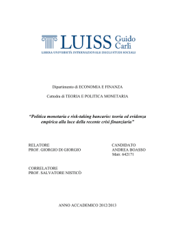
behavior of the common factors and their loadings. In order to do so, we first run a CUSUM
Square test on the common factors (Brown et al., 1975) and find no significant structural
change (Figure 1). Then, we run the structural break test of Breitung and Eickmeier (2011)
on the factor loadings, which indicates structural break on January the 1st 1999 for all the
series of interest (Table 1). These results are consistent with Canova et al. (2012) and Breitung
and Eickmeier (2011).
2.2
Testing for asymmetries
In order to evaluate the presence of significant differences across impulse responses we should
test the null-hypothesis of no differences. Olivei and Tenreyro (2010) propose a procedure to
test for differences among impulse responses in VAR models. Their test consists in computing
differences among observed impulse responses and then compare them with a distribution of
distances obtained from data simulated from two different VARs. Unfortunately, this test is
unfeasible in our case. Indeed, while Olivei and Tenreyro (2010) aim at comparing impulse
responses of the same variable, but estimated from two different (VAR) models, we are interested in comparing responses of different variables, but estimated from the same (factor)
model. Hence, in our case we should be able to simulate data from a factor model in which
all impulse responses are equal. Building such a distribution would lead to a degenerate distribution in which all distances among impulse responses are zero, i.e. a useless distribution
for making inference.
Therefore, in order to have an approximate measure of asymmetries, we rely on a simple
procedure with a clearly intuitive meaning. In particular, for each bootstrap, we compute the
difference between the individual country response and the Euro Area response. These gives
us a distribution of differences between impulse responses. We consider the difference non
significant if zero is contained within the confidence bands.9 A similar procedure is used also
by Fielding and Shields (2011).
3
Model setup
3.1
Data and data treatment
Data include EA aggregates, main macroeconomic variables for single EA member states, and
key indicators for the United Kingdom, the United States, and Japan. The database contains
9 aggregate EA variables: GDP, CPI, short and long term rates, monetary aggregates (M1 and
M3), unit labor cost, real effective exchange rate, and the dollar/euro exchange rate. These
9
We would like to thank an anonymous referee for suggesting us this testing procedure.
9
aggregate variables are taken either from Eurostat, or from ECB, and, when necessary, they
are backdated by using data from the Area Wide Model Database (Fagan et al., 2001).
We then have 35 variables for Germany, Italy, and the Netherlands, 34 for France and
Spain, and 31 for Belgium. Variables included for these countries are: interest rates, monetary
aggregates, real effective exchange rate, an index of stock prices, GDP and its expenditure
components, unemployment rate, unit labor costs, GDP deflator, producer price index, CPI
together with its disaggregated categories, retail sales, and number of cars sold. In addition, we
also include CPI, GDP, and interest rates for smaller EA countries (Finland, Greece, Ireland,
Luxembourg, and Portugal), and for UK, US, and Japan, as well as the spot oil price.
Summing up, our datasets consists of 237 quarterly time series covering the period 1983Q1–
2007Q4.10 The complete list of variables, sources, and the transformations used is available
in the Supplementary Appendix.
A comment is necessary on the way we transform data in order to make them stationary. According to Uhlig (2009), the co-movements found by Boivin et al. (2009) in a similar
dataset, are actually the result of the autocorrelation induced in the transformed data. As a
consequence, the existence of a factor structure, based on co-movements among series, would
be just a by-product of data treatment. In order to cope with this critique, and compared
with Boivin et al. (2009), we adopt a different set of transformations. As in Stock and Watson
(2005) and Forni and Gambetti (2010c), we take second differences of the log of both prices
and monetary aggregates, first differences of interest rates, and, when needed, growth rates are
computed on a quarterly basis.11 We label this kind of transformations as heavy, in contrast
with light transformations used by Boivin et al. (2009). In the latter case interest rates are
kept in levels, the first difference of log of prices and monetary aggregates is taken, and, most
importantly, growth rates are computed on a yearly basis.
With reference to Uhlig (2009) critique, our choice of heavy transformations is justified
by Table 2, where we report selected percentiles of the distribution of the absolute value of
univariate autocorrelations when considering light vs. heavy transformations. The median
autocorrelation from lags 1 to 4 is between 0.36 and 0.15 in the heavy case, while it is between
0.86 and 0.28 in the light case. Similar results hold also for other percentiles.
3.2
Number of common shocks and factors
After transforming data, we rely on specific tests and information criteria for determining the
number of common factors r and common shocks q. The latter is estimated by means of the
test proposed by Onatski (2009), which suggests q ∈ {4, 5} (Table 3) and the criterion by
Hallin and Liška (2007) suggesting q ∈ {2, 3}. We choose as our baseline specification q = 4,
i.e. the average of these results.12
10
The sample starts in 1983 because of two main reasons. First, not all the series in the database, especially
at the single European country level, are available before 1983. Second, although EA data at the aggregate
level are available since 1970 at a quarterly frequency, by comparing alternative aggregation methods, Bosker
(2006) shows that differences in EA artificial data are prominent before 1983 especially for inflation and interest
rates, while vanishing thereafter.
11
It is worth to note that, within the literature on money demand in the EA (Papademos and Stark, 2010,
and reference therein), it is common practice to treat monetary aggregates as I(2) variables. Furthermore,
Beyer (2009) and Dreger and Wolters (2010), among others, show that inflation is an important determinant
in describing a stable long run money demand equation for the EA, thus indicating that money growth and
inflation are cointegrated, and therefore I(1) variables.
12
It is also worth noting that four common shocks is a parameterization considered plausible in the literature.
In particular, in her discussion of Boivin et al. (2009), Reichlin (2009) rises some doubts about their choice
10
One possible way of fixing the number of common factors is to choose r such that the
variance explained by the factors is equal to the variance explained by the chosen q shocks.
This heuristic method suggests 13 factors (see Table 5). An alternative is to resort to the
criterion provided by Bai and Ng (2002), and its refinement by Alessi et al. (2010), both
suggesting either 9 or 14 factors. We choose as our baseline specification r = 12, i.e. the
average of what the mentioned criteria suggest.13
In Table 4 we show the share of variance accounted for by the estimated common component. When looking at the post-1999 sample, we find that 91% of aggregate GDP and 90% of
aggregate CPI fluctuations are imputable to the common component. These values decrease
if we look at country specific GDP, CPI, and unemployment rate, but are still considerably
high in the majority of the cases, notwithstanding the heterogeneity and large dimension of
the dataset at hand. Indeed, the variance of the common component is more than 60% of
total GDP fluctuations for all countries but Belgium (59%), Finland (54%), Portugal (45%),
Greece (44%), and Ireland (12%), while it is more than 70% of total CPI fluctuations for
all countries but Portugal (70%), Finland (60%), and Greece (54%), and more than 50% of
total unemployment fluctuations for all countries but Belgium (47%) and Italy (36%). When
averaging common variances across all 237 considered variables, we have that the common
component accounts for 51% of the total fluctuations.
The existence of cross-country heterogeneity in the co-movements both justifies our approach (co-movements imply a factor structure), and motivates our research question (heterogeneity suggests asymmetric reactions).
4
Identification of the monetary policy shock
We identify the monetary policy shock by means of sign restrictions (Faust, 1998; Canova
and de Nicolò, 2002; Uhlig, 2005), an identification strategy also used in the context of factor
models by Eickmeier (2009) and Forni and Gambetti (2010b,c). Specifically, at each iteration
we draw a vector of q(q − 1)/2 angles ω from a uniform distribution on [0, 2π), which, by
means of Givens transform, are used to construct an orthogonal matrix R(ω) of dimension
q × q. We then compute the associated impulse responses and if they satisfy a prescribed set
of sign restrictions (to be specified below) we accept the draw, otherwise we discard it. We
stop this procedure once K draws are accepted.
We rely on the following assumptions imposed only on EA variables for the first two lags:
after a contractionary monetary policy shock the short term interest rate, the real effective
exchange rate, and the dollar/euro exchange rate increase, while GDP, CPI, and M1 decrease.
These restrictions, which are theoretically consistent with a typical IS-LM model of an open
economy, are commonly accepted in the literature (Peersman, 2005; Farrant and Peersman,
2006). Moreover, the choice of imposing restrictions only on the EA variables makes the
identification scheme “agnostic” on the responses of single countries (see also Eickmeier, 2009,
for a similar identification scheme).
of seven common shocks by arguing that a smaller number of common shocks would be much more plausible: “when macroeconomists think of common shocks, they mention productivity, money, time preference, or
government, and it is difficult to think of many other candidates” (p. 130).
13
Other criteria, not used in this paper, to determine q or r are in Bai and Ng (2007), Amengual and Watson
(2007), Onatski (2010), and Kapetanios (2010). Results for the criteria by Bai and Ng (2002), Hallin and Liška
(2007), and Alessi et al. (2010), as well as robustness analysis for for q = {3, 5} and r = {9, 13}, are available
in the Supplementary Appendix to this paper.
11
The choice of an “agnostic” identification scheme leaves the room open to non-conventional
reactions (see Section 5). Therefore, we also tried to impose country specific restrictions, but
we did not find rotation matrices able to satisfy all the restrictions. This result has an economic
interpretation as discussed in Sections 5 and 6. In particular, we are able to satisfy some of,
but not all, the country specific restrictions. More specifically, restrictions on GDP are easily
satisfied, but for Greece in the 1983-1998 sample, whereas restrictions for prices are satisfied
only for Belgium, France, Germany, and the Netherlands. There are very few rotations that
satisfy the restrictions for prices in Spain and in Italy, but almost no rotations that satisfy
the restrictions jointly for Italy and Spain. For Finland, Greece and Ireland we cannot find
restrictions for the pre-euro sample, while for Portugal we cannot find them for the post euro
sample. Finally, it is worth noting that unconventional reactions of inflation or prices to the
monetary policy shock are also found by Sala (2003) for Italy and Portugal, Eickmeier (2009)
for Greece and Portugal, Boivin et al. (2009) for Germany, and Peersman (2004) for Austria
and Italy.
In order to compute impulse responses and the related confidence intervals, we use the
procedure described in Section 2 with 500 bootstrap draws. To keep computations feasible,
for each of the 500 + 1 samples we save K = 10 rotation matrices. Then, for each sample we
select just one rotation matrix as suggested by Fry and Pagan (2011).14
An alternative strategy to identify monetary policy is to adopt a recursive identification
scheme, i.e. the Cholesky decomposition as in Boivin et al. (2009) and Forni and Gambetti
(2010a). Although recently criticized (Canova and Pina, 2005; Carlstrom et al., 2009; Uhlig,
2009; Castelnuovo, 2011, 2012a), this is the simplest, and perhaps, still, the most diffused
identification scheme in SVAR literature (Christiano et al., 1999; Peersman and Smets, 2003;
Weber et al., 2011). The main problem of this identification scheme is that it relies on zero
short-run restrictions, which are too binding and not necessarily based on economic theory.
Differently, by using sign restrictions, we are imposing restrictions often used implicitly in
empirical analysis to validate the results, and consistent with macroeconomic models. However, if the shock of interest explains a marginal fraction of the forecast error of the variables
of interest, the outcome of the exercise conducted with sign restrictions should also be taken
cautiously (for a Monte Carlo experiment, see Paustian, 2007; Castelnuovo, 2012b). For these
reasons, in the Supplementary Appendix we show also results obtained with Cholesky identification.
5
Results
In this Section, we present impulse response functions to a monetary policy shock. The shock
is normalized so that on impact it raises EA short term rate of 50 basis points. In Figures
2-7, we show the impulse responses of CPI, GDP, together with consumption and investment,
and unemployment rate both at the aggregate level, and at the country level. Each Figure
contains the impulse responses, together with 68% confidence bands, estimated both on the
pre-euro sample (grey solid line, and shaded area), and on the euro-sample (black solid and
dashed lines).
14
Fry and Pagan (2011) point out that for each sample the distribution of the R(ω) that satisfies the sign
restrictions represents model uncertainty. However, when computing impulse responses with confidence bands
what matters is sampling uncertainty, not model uncertainty. Hence they suggest selecting for each sample
just one rotation, namely the one which produces the impulse response closest to the median response.
12
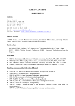
Figure 2 shows impulse responses for the aggregate EA variables used in the identification
of the monetary policy shock and it should be considered just as validation of our identification
strategy. In both samples, output, prices, and the monetary aggregate M1 respond negatively,
while the short term rate and exchange rates respond positively. Notice that we estimate a
strong effect of monetary policy shocks on the economy (in particular on both GDP and CPI).15
However, our estimates are not far from those usually found by the literature (Monticelli and
Tristani, 1999; Sala, 2003; Eickmeier, 2009).16
When comparing pre-euro with euro sample impulse responses of aggregate CPI and GDP,
we find that the introduction of the common currency amplified the response of CPI, while
reducing the reaction of GDP. This result is consistent with an increase in prices’ flexibility
due to greater competition between EA industries.17
We then move to the analysis of country specific variables. In Figure 8 we show results of
the test on the asymmetries introduced in Section 2.2. In each plot of Figure 8 the grey/black
straight line is the median difference between the response of a given country and the response
of a benchmark country, while the shaded area/dashed lines is/are the 68% confidence bands
estimated on the pre-euro/euro sample. If at horizon h the zero is contained within the confidence bands, it means that the impulse response of a given country and that of a benchmark
country are not statistically different at horizon h. In panels (a) and (b) the benchmark
country is the EA, while in panels (c), (d), and (e) the benchmark country is Germany.
The goal is to understand whether there are asymmetries in the transmission mechanism
of the common monetary policy to EA countries before and after 1999, and to understand
which was the effect, if any, of the common monetary policy on the existing asymmetries.
Notice also that, in terms of our research question what matters is the direction (i.e. signs)
and the significance of the cross-country differences rather than the magnitudes, which turn
out to be implausibly high for some of the countries.
5.1
Cross-country differences before 1999
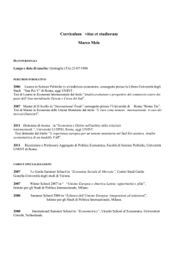
Prices. Four countries out of ten (Finland, Italy, Portugal, and Greece) exhibit a positive
reaction (Figure 3). In addition to the four countries just mentioned, also the impulse responses
of France, Belgium, and the Netherlands are statistically different from those of the EA (Figure
8.a) thus showing a high degree of pre-euro heterogeneity in prices.
GDP. All countries, but Greece, react as predicted by economic theory (Figure 4). The
unconventional response of Greece seems to be related with the low percentage of variance of
Greek GDP explained by the common component (see Table 4). Indeed, it should be noted
that Greece was not part of the European Monetary System, as it only joined it in stage II,
i.e. in 1999. When testing for asymmetries (Figure 8.b) we find that also the reactions of
15
The reason for these large magnitudes in the response of prices comes from the heavy transformations
choice. In particular, since we model CPI as an I(2) process, we obtain explosive dynamics due to the need of
cumulating twice the estimated IRF.
16
Detailed information on the magnitude of the impulse responses estimated by the literature cited in this
paper can be found in the Supplementary Appendix.
17
It may be argued that, since before 1999 there was no common monetary policy, the relevant comparison
would be between pre–1999 Bundesbank monetary policy, and post–1999 ECB monetary policy (Sala, 2003).
Hence, as a robustness check we estimated our model by imposing in the pre–1999 sample the identifying
restrictions on the German short term interest rate. Results are near identical to the one obtained with our
benchmark specification, and are available in the Supplementary Appendix to this paper.
13
Germany, the Netherlands, Italy, Spain, Ireland, and Portugal are statistically different than
those of the EA thus showing a high degree of heterogeneity pre-euro in output.
Consumption. All countries display the expected negative path (Figure 5). However, when
testing for asymmetries (Figure 8.c) some differences emerge since both France and the Netherlands react significantly less than Germany, while Italy and Spain react significantly more.
Investment. All countries react as predicted by economic theory (Figure 6) and all react
significantly differently than Germany (Figure 8.d).
Unemployment Rate. Unemployment in Germany, France, the Netherlands, and Belgium
follows a similar hump–shaped path, while impulse responses for Spain and Italy are different
(Figure 7). However, when testing for asymmetries (Figure 8.e) we find that also France and
the Netherlands react in a significantly different way than Germany.
5.2
Cross-country differences after 1999
Prices. We can divide EA countries in three groups (see Figure 3). In the first, we have
countries for which we observe the expected negative response to the common monetary policy
shock: Germany, France, the Netherlands, and Finland. In the second group, we have countries
for which we estimate a mute response (i.e. not significantly different from zero): Ireland,
Belgium, Spain, Italy, and Greece. Finally, the third group is composed of a single country for
which we estimate a positive response, namely Portugal (see also Sala, 2003; Eickmeier, 2009).
If we consider these results with reference to pre-euro impulse responses, the introduction of a
common currency appears to have had a positive role in shaping homogeneity across countries
CPIs. Table 4 provides an explanation of this switch in terms of explained variances of the
common components: the higher this number, the more impulse responses are homogeneous.
However, significant asymmetries persist between the EA and Finland, Italy, Portugal and
Greece (Figure 8.a), with Finland reacting more than the EA, and Italy, Portugal, and Greece
reacting less. The response of the Mediterranean countries seems likely to be the consequence
of price rigidities and of lack of competition.
GDP. Impulse responses are quite similar across countries (Figure 4). With respect to the
pre-euro sample, the response of Greek GDP has now the expected negative sign. Overall, the
introduction of the euro has helped in reducing asymmetries. However, small differences are
still present between the EA and the Netherlands, Ireland, and Portugal (Figure 8.b). While
Ireland and Portugal GDP fluctuations are mainly idiosyncratic (Table 4), the strong reaction
of Dutch GDP seems to be driven by consumption.
Consumption. The Netherlands and Italy display the deepest reaction in consumption with
a minimum of roughly -5% and -3% respectively (Figure 5), a result also found by Reichlin
(2009) in the case of Italy. The response of Netherlands consumption is likely due to the
particular dynamics of the series, which has nothing to do with monetary policy. Indeed, from
1999 to 2003 the year on year consumption growth trended downward as a consequence of
firms’ and households’ balance sheets adjustments, weak profits, and lower purchasing power of
households. Germany, Belgium and Spain also show a significant contraction in consumption
up to -1%, while the response is mute for France. The introduction of the euro has slightly
reduced asymmetries for Italy and Spain (Figure 8.c).
14
Investment. The reaction of investment is more homogeneous with the main exception of
Germany for which a contraction up to -9% is observed (Figure 6). This result is likely due to
the dynamics of the German construction sector, as the housing market was characterized by a
post-reunification boom-bust cycle in residential investment (Knetsch, 2010). This anomalous
response of Germany implies significant differences with respect to all other countries (Figure
8.d), which, however, have all similar responses.
Unemployment Rate. As in the pre-euro sample, all countries but Italy and Spain show
similar reactions (Figure 7). However, asymmetries are reduced between Germany and France
and the Netherlands (Figure 8.e). More specifically, on the one hand Spanish unemployment
rate experiments a stronger boost than other countries, on the other hand, Italian unemployment seems not to respond to a common monetary policy shock. The first finding suggests
large elasticity of Spanish labor market to monetary policy shocks likely due to the high share
of fixed term contracts in the labor market (see for example Güell and Petrongolo, 2007).
In contrast, the mute response of Italian unemployment is the consequence of a rigid labor
market which seems not to be related at all to the business cycle as confirmed from the low
correlation (-0.07) between changes in unemployment rate and GDP growth.18
6
Discussion and conclusions
In this paper we ask the following question: is there any asymmetry in how single EA countries
respond to the common monetary policy decided by the ECB?
In order to answer we estimate a Structural Dynamic Factor model on a large panel of EA
quarterly time series spanning the period from 1983 to 2007. The dataset incorporates data
on the aggregate EA as well as country-specific key economic variables, such as gross domestic
product, inflation, unemployment, consumption, investment, and many others.
We find that, although the introduction of the euro has changed the monetary transmission
mechanism in the individual countries towards a more homogeneous response, differences still
remain between North and South Europe in terms of prices and unemployment. Due to their
idiosyncratic nature, these differences can hardly be controlled by means of the common monetary policy; rather they should be addressed by means of national fiscal policies, regulation,
and structural reforms. Indeed, while before 1999 CPI responses were highly asymmetric, the
introduction of the euro and of the single monetary policy, and the consequent increase in
integration and competition within the EA, made prices more flexible thus responding more
homogeneously to changes in interest rate. The remaining asymmetries are observed in the
Mediterranean countries, which historically have less flexible prices and lack of market competition. Similarly, the asymmetries in labor markets seem to be the result of structural and
socio-economic characteristics of single countries. This is the case for example with the rigid
labor market structure in Italy, which makes Italian unemployment rate essentially unresponsive to the single monetary policy.
In conclusion, EA countries react asymmetrically to the common monetary policy in terms
of prices and unemployment, while no difference appears in terms of output. While the post1999 reduction in asymmetries is consistent with the aims of the ECB (see Boivin et al.,
2009), the remaining differences are beyond the scope of monetary policy, and they should be
18
Correlations for other countries are: Belgium -0.27, France -0.36, Germany -0.29, the Netherlands -0.26,
and Spain -0.34.
15
addressed by means of national reforms. As demonstrated by the recent/current public debt
crisis, and by the skyrocketing of government bond spreads, these differences pose a threat to
the region’s stability: addressing them is fundamental for the future of Europe, and it should
be a priority if economic cohesion is to be achieved.
16
References
Alessi, L., M. Barigozzi, and M. Capasso (2010). Improved penalization for determining the
number of factors in approximate static factor models. Statistics and Probability Letters 80,
1806–1813.
Amengual, D. and M. W. Watson (2007). Consistent estimation of the number of dynamic
factors in a large N and T panel. Journal of Business and Economic Statistics 25, 91–96.
Bai, J. (2003). Inferential theory for factor models of large dimensions. Econometrica 71,
135–171.
Bai, J. and S. Ng (2002). Determining the number of factors in approximate factor models.
Econometrica 70, 191–221.
Bai, J. and S. Ng (2006). Confidence Intervals for Diffusion Index Forecasts and Inference for
Factor-Augmented Regressions. Econometrica 74, 1133–1150.
Bai, J. and S. Ng (2007). Determining the number of primitive shocks in factor models.
Journal of Business and Economic Statistics 25, 52–60.
Bernanke, B. S., J. Boivin, and P. S. Eliasz (2005). Measuring the effects of monetary policy:
A Factor-Augmented Vector Autoregressive (FAVAR) approach. The Quarterly Journal of
Economics 120, 387–422.
Beyer, A. (2009). A stable model for Euro Area money demand: Revisiting the role of wealth.
Working Paper Series 1111, European Central Bank.
Boivin, J., M. Giannoni, and B. Mojon (2009). How has the euro changed the monetary
transmission mechanism? In D. Acemoglu, K. Rogoff, and M. Woodford (Eds.), NBER
Macroeconomics Annual 2008. University of Chicago Press.
Bosker, E. (2006). On the aggregation of eurozone data. Economics Letters 90 (2), 260–265.
Breitung, J. and S. Eickmeier (2011). Testing for structural breaks in dynamic factor models.
Journal of Econometrics 163, 71–84.
Brown, R. L., J. Durbin, and J. M. Evans (1975). Techniques for testing the constancy of
regression relationships over time. Joumal of the Royal Statistical Society, Series B 37,
149–192.
Canova, F., M. Ciccarelli, and E. Ortega (2012). Do institutional changes affect business
cycles? Evidence from Europe. Journal of Economic Dynamics and Control 36, 1520–1533.
Canova, F. and G. de Nicolò (2002). Monetary disturbances matter for business fluctuations
in the G-7. Journal of Monetary Economics 49 (6), 1131–1159.
Canova, F. and J. P. Pina (2005). What VAR tell us about DSGE models. In C. Diebolt and
C. Kyrtsou (Eds.), New Trends In Macroeconomics. New York: Springer Verlag.
Carlstrom, C. T., T. S. Fuerst, and M. Paustian (2009). Monetary policy shocks, Choleski
identification and DNK models. Journal of Monetary Economics 56, 1014–1021.
17
Castelnuovo, E. (2011). Monetary policy shocks and Cholesky-VARs: An assessment for the
Euro Area. University of Padua, mimeo.
Castelnuovo, E. (2012a). In Cholesky–VARs we trust? An empirical investigation for the U.S.
University of Padua, mimeo.
Castelnuovo, E. (2012b). Monetary policy neutrality? Sign restrictions go to Monte Carlo.
University of Padua, mimeo.
Cecioni, M. and S. Neri (2011). The monetary transmission mechanism in the euro area: has
it changed and why? Temi di discussione (Economic working papers) 808, Bank of Italy,
Economic Research and International Relations.
Chamberlain, G. and M. Rothschild (1983). Arbitrage, factor structure, and mean-variance
analysis on large asset markets. Econometrica 51 (5), 1281–304.
Christiano, L. J., M. Eichenbaum, and C. L. Evans (1999). Monetary policy shocks: What
have we learned and to what end? In J. B. Taylor and M. Woodford (Eds.), Handbook of
Macroeconomics, Volume 1, pp. 65–148. Elsevier.
Ciccarelli, M. and A. Rebucci (2006). Has the transmission mechanism of European monetary
policy changed in the run-up to EMU? European Economic Review 50, 737–776.
Clarida, R., J. Galí, and M. Gertler (1998). Monetary policy rules in practice: Some international evidence. European Economic Review 42 (6), 1033–1067.
Clements, B., Z. G. Kontolemis, and J. Levy (2001). Monetary policy under EMU: Differences
in the transmission mechanism? Working Paper 102, International Monetary Fund.
Doz, C., D. Giannone, and L. Reichlin (2011). A two-step estimator for large approximate
dynamic factor models based on Kalman filtering. Journal of Econometrics 164, 188–205.
Doz, C., D. Giannone, and L. Reichlin (2012). A quasi maximum likelihood approach for large
approximate dynamic factor models. Review of Economics and Statistics 94, 1014–1024.
Dreger, C. and J. Wolters (2010). Investigating M3 money demand in the Euro Area. Journal
of International Money and Finance 29, 111–122.
Durbin, J. (1969). Tests for serial correlation in regression analysis based on the periodogram
of least squares residuals. Biometrika 56, 1–15.
Edgerton, D. and C. Wells (1994). Critical values for the CUSUMSQ statistic in medium and
large sized samples. Oxford Bulletin of Economics and Statistics 54, 355–365.
Eickmeier, S. (2009). Comovements and heterogeneity in the Euro Area analyzed in a nonstationary dynamic factor model. Journal of Applied Econometrics 24, 933–959.
Eickmeier, S. and J. Breitung (2006). How synchronized are new EU member states with the
Euro Area? Evidence from a structural factor model. Journal of Comparative Economics 34,
538–563.
Fagan, G., J. Henry, and R. Mestre (2001). An area-wide model (AWM) for the Euro Area.
Working Paper 42, European Central Bank.
18
Farrant, K. and G. Peersman (2006). Is the exchange rate a shock absorber or a source of
shocks? New empirical evidence. Journal of Money, Credit and Banking 38, 939–961.
Faust, J. (1998). The robustness of identified VAR conclusions about money. CarnegieRochester Conference Series on Public Policy 49, 207–244.
Favero, C. A., M. Marcellino, and F. Neglia (2005). Principal components at work: The empirical analysis of monetary policy with large datasets. Journal of Applied Econometrics 20,
603–620.
Fielding, D. and K. Shields (2011). Regional asymmetries in the impact of monetary policy
shocks on prices: Evidence from US cities. Oxford Bulletin of Economics and Statistics 73,
79–103.
Forni, M. and L. Gambetti (2010a). The dynamic effects of monetary policy: A structural
factor model approach. Journal of Monetary Economics 57, 203–216.
Forni, M. and L. Gambetti (2010b). Fiscal foresight and the effects of goverment spending.
Discussion Papers 7840, C.E.P.R.
Forni, M. and L. Gambetti (2010c). Macroeconomic shocks and the business cycle: Evidence
from a structural factor model. Discussion Papers 7692, C.E.P.R.
Forni, M., D. Giannone, M. Lippi, and L. Reichlin (2009). Opening the black box: Structural
factor models versus structural VARs. Econometric Theory 25, 1319–1347.
Forni, M., M. Hallin, M. Lippi, and L. Reichlin (2000). The generalized dynamic factor model:
Identification and estimation. The Review of Economics and Statistics 82, 540–554.
Forni, M. and M. Lippi (2001). The generalized dynamic factor model: Representation theory.
Econometric Theory 17, 1113–1141.
Fry, R. and A. R. Pagan (2011). Sign restrictions in structural vector autoregressions: A
critical review. Journal of Economic Literature 49, 938–960.
Geweke, J. (1977). The dynamic factor analysis of economic time series. In D. J. Aigner and
A. S. Goldberger (Eds.), Latent Variables in Socio-Economic Models. Amsterdam: North
Holland.
Giannone, D., L. Reichlin, and L. Sala (2005). Monetary policy in real time. In M. Gertler
and K. Rogoff (Eds.), NBER Macroeconomics Annual 2004. MIT Press.
Güell, M. and B. Petrongolo (2007). How binding are legal limits? Transitions from temporary
to permanent work in Spain. Labour Economics 14, 153–183.
Hallin, M. and R. Liška (2007). Determining the number of factors in the general dynamic
factor model. Journal of the American Statistical Association 102, 603–617.
Kapetanios, G. (2010). A testing procedure for determining the number of factors in approximate factor models with large datasets. Journal of Business and Economic Statistics 28,
397–409.
19
Kilian, L. (1998). Small-sample confidence intervals for impulse response functions. Review
of Economics and Statistics 80, 218–230.
Knetsch, T. A. (2010). Trend and cycle features in German residential investment before and
after reunification. In O. Bandt, T. Knetsch, J. Peñalosa, and F. Zollino (Eds.), Housing
Markets in Europe, pp. 187–211. Springer Berlin Heidelberg.
Luciani, M. (2012). Monetary policy and the housing market: A structural factor analysis.
Journal of Applied Econometrics. forthcoming.
McCallum, A. and F. Smets (2009). Real wages and monetary policy transmission in the
Euro Area. University of Michigan and ECB, mimeo. Paper presented at ECB conference
on Monetary policy transmission mechanism in the Euro Area in its first 10 years, Frankfurt,
September 2009.
Mihov, I. (2001). Monetary policy implementation and transmission in the european monetary
union. Economic Policy 16 (33), 369–406.
Mojon, B. and G. Peersman (2003). The monetary transmission mechanism in the Euro Area:
More evidence from VAR models? In I. Angeloni, A. K. Kashyiap, and B. Mojon (Eds.),
Monetary Policy Transmission in the Euro Area. Cambridge University Press.
Monticelli, C. and O. Tristani (1999). What does the single monetary policy do? A SVAR
benchmark for the European Central Bank. Working Paper 2, European Central Bank.
Olivei, G. and S. Tenreyro (2010). Wage-setting patterns and monetary policy: International
evidence. Journal of Monetary Economics 57, 785–802.
Onatski, A. (2009). Testing hypotheses about the number of factors in large factor models.
Econometrica 77, 1447–1479.
Onatski, A. (2010). Determining the number of factors from empirical distribution of eigenvalues. Review of Economics and Statistics 92, 1004–1016.
Papademos, L. D. and J. Stark (Eds.) (2010). Enhancing Monetary Analysis. European
Central Bank.
Paustian, M. (2007). Assessing sign restrictions. The B.E. Journal of Macroeconomics 7 (1),
1–33.
Peersman, G. (2004). The transmission of monetary policy in the Euro Area: Are the effects
different across countries? Oxford Bulletin of Economics and Statistics 66, 285–308.
Peersman, G. (2005). What caused the early millennium slowdon? Evidence based on vector
autoregressions. Journal of Applied Econometrics 20, 185–207.
Peersman, G. and F. Smets (2003). The monetary transmission mechanism in the Euro Area:
More evidence from VAR analysis. In I. Angeloni, A. K. Kashyiap, and B. Mojon (Eds.),
The Monetary Transmission Mechanism in the Euro Area. Cambridge University Press.
Rafiq, M. S. and S. K. Mallick (2008). The effects of monetary policy on output in EMU: A
sign restrictions approach. Journal of Macroeconomics 30, 1756–1791.
20
Reichlin, L. (2009). Comment on “How has the Euro changed the monetary transmission”;.
In D. Acemoglu, K. Rogoff, and M. Woodford (Eds.), NBER Macroeconomics Annual.
University of Chicago Press.
Sala, L. (2003). Monetary transmission in the Euro Area: A factor model approach. University
Bocconi.
Sargent, T. J. and C. A. Sims (1977). Business cycle modeling without pretending to have
too much a-priori economic theory. In C. A. Sims (Ed.), New Methods in Business Cycle
Research. Minneapolis: Federal Reserve Bank of Minneapolis.
Stock, J. H. and M. W. Watson (2002). Forecasting using principal components from a large
number of predictors. Journal of the American Statistical Association 97, 1167–1179.
Stock, J. H. and M. W. Watson (2005). Implications of dynamic factor models for VAR
analysis. Working Paper 11467, NBER.
Uhlig, H. (2005). What are the effects of monetary policy on output? Results from an agnostic
identification procedure. Journal of Monetary Economics 52, 381–419.
Uhlig, H. (2009). Comment on “How has the Euro changed the monetary transmission”;.
In D. Acemoglu, K. Rogoff, and M. Woodford (Eds.), NBER Macroeconomics Annual.
University of Chicago Press.
Weber, A. A., R. Gerke, and A. Worms (2011). Changes in euro area monetary transmission?
Applied Financial Economics 21, 131–145.
21
Tables
Table 1: Testing for Structural Break in the Factor Loadings:
Breitung and Eickmeier Test
Consumer Price Index
Gross Domestic Product
Consumption
Investment
Unemployment Rate
BG
63.44
81.41
70.35
49.91
66.52
FR
71.35
74.14
55.96
66.55
55.61
GE
72.50
76.29
65.19
52.65
34.15
IT
55.46
54.57
66.52
51.76
47.61
NL
60.86
58.66
34.19
48.81
54.45
ES
63.32
79.83
56.59
68.91
48.21
FI
41.56
70.87
GR
37.75
30.82
IE
48.56
39.30
PT
57.69
45.10
EA
80.68
88.59
This Table show the LM Statistic for the null of no structural break in the factor loadings on January the 1st 1999. This statistic
is asymptotically distributed as a χ2 random variable with r (number of factors degrees of freedoms. The 10%, 5%, and 1% critical
values are 18.5493, 21.0261, and 26.2170 respectively.
Table 2: The Distribution of Autocorrelations
Light vs. Heavy
Percentile
light
5
25
50
75
95
heavy
5
25
50
75
95
1
0.65
0.81
0.86
0.90
0.95
1
0.08
0.24
0.36
0.54
0.90
2
0.40
0.57
0.67
0.78
0.87
2
0.02
0.09
0.18
0.32
0.74
3
0.12
0.32
0.47
0.65
0.78
3
0.01
0.06
0.15
0.27
0.59
Lag
4
0.03
0.11
0.28
0.51
0.70
4
0.01
0.07
0.15
0.25
0.50
5
0.03
0.13
0.23
0.43
0.64
5
0.01
0.06
0.14
0.23
0.39
6
0.04
0.12
0.22
0.36
0.58
6
0.01
0.04
0.11
0.18
0.35
7
0.02
0.09
0.19
0.32
0.54
7
0.01
0.04
0.10
0.18
0.30
8
0.02
0.07
0.16
0.29
0.51
8
0.01
0.04
0.10
0.16
0.33
Percentiles of the distribution of univariate autocorrelation functions when computing
light transformations as in Boivin et al. (2009) or heavy transformations, i.e. by replacing
yearly with quarterly growth rates and taking first differences of interest rates and second
differences of the log of prices and monetary aggregates.
22
Table 3: Determining the Number of Common Shocks:
Onatski Test
1
0.029
q0 vs. q1
0
1
2
3
4
5
6
7
2
0.050
0.271
3
0.069
0.487
0.608
4
0.088
0.626
0.677
0.390
5
0.104
0.321
0.262
0.195
0.108
6
0.121
0.372
0.321
0.262
0.195
0.947
7
0.135
0.421
0.372
0.321
0.262
0.923
0.623
8
0.151
0.465
0.421
0.372
0.321
0.343
0.257
0.142
This Table shows p-values of the null of q0 common shocks against the alternative of q0 <
q ≤ q1 common shocks. The Discrete Fourier Transformation of the data is computed for
ωj = 2πsj /T , with sj ∈ [2, ..., 20], thus to includes waves between 1 and 12 years.
Table 4: Comovements in the Euro Area
Explained Variance
Country
Euro Area
Germany
France
Netherlands
Belgium
Finland
Italy
Spain
Portugal
Ireland
Greece
GDP
83-98 99-07
0.85
0.91
0.71
0.76
0.74
0.78
0.31
0.73
0.66
0.59
0.63
0.54
0.42
0.66
0.38
0.66
0.67
0.45
0.39
0.12
0.20
0.44
CPI
83-98 99-07
0.79
0.90
0.69
0.80
0.49
0.82
0.73
0.75
0.55
0.81
0.31
0.60
0.70
0.82
0.62
0.90
0.51
0.70
0.33
0.72
0.18
0.54
UR
83-98 99-07
0.48
0.69
0.55
0.60
0.54
0.58
0.58
0.47
0.50
0.36
0.67
0.57
-
For each country we report the variance explained by the common component
of GDP, CPI, and Unemployment Rate (UR). For each variable the first column
refers to the 1983:Q1-1998:Q4 (pre-euro) sample, and the second column to the
1999:Q1-2007:Q4 (euro) sample. Values are given on a scale between 0 (no
contribute of the common component) and 1.
Table 5: Cumulated Explained Variance:
q
r
1
0.21
0.09
2
0.34
0.16
3
0.43
0.23
4
0.51
0.27
5
0.58
0.31
Number of Factors
6
7
8
9
0.64 0.68 0.73 0.76
0.34 0.37 0.40 0.42
10
0.79
0.45
11
0.82
0.47
12
0.84
0.49
13
0.86
0.51
14
0.88
0.53
The Table shows the percentage of overall variance explained by the first q common shocks estimated with the method of dynamic
principal components as in Forni et al. (2000), and the first r static factors estimated by static principal components. Variance is
measured on a scale between 0 and 1.
23
Figures
Figure 1: CUSUM Square Test on the Static Factors
0.3
0.3
0.3
0.3
0.2
0.2
0.2
0.2
0.1
0.1
0.1
0.1
0
0
0
0
−0.1
−0.1
−0.1
−0.1
−0.2
1990
−0.2
1995
2000
2005
1990
−0.2
1995
2000
2005
1990
−0.2
1995
2000
2005
1990
0.3
0.3
0.3
0.3
0.2
0.2
0.2
0.2
0.1
0.1
0.1
0.1
0
0
0
0
−0.1
−0.1
−0.1
−0.1
−0.2
1990
−0.2
1995
2000
2005
1990
−0.2
1995
2000
2005
1990
2000
2005
1990
0.3
0.3
0.3
0.2
0.2
0.2
0.2
0.1
0.1
0.1
0.1
0
0
0
0
−0.1
−0.1
−0.1
−0.1
1990
−0.2
1995
2000
2005
1990
−0.2
1995
2000
2005
1990
2000
2005
1995
2000
2005
1995
2000
2005
−0.2
1995
0.3
−0.2
1995
−0.2
1995
2000
2005
1990
Solid line is the CUSUM Square statistic of (Brown et al., 1975), while the dashed lines
are the 90% confidence bands computed using critical values as given in Durbin (1969)
and Edgerton and Wells (1994).
24
Figure 2: Impulse Responses to a Monetary Policy Shock
Euro Area Aggregates
GDP
CPI
0
5
−1
0
−2
−5
−3
−10
−4
0
5
10
15
20
0
5
M1
10
15
20
Short Term Interest Rate
40
0
20
−1
0
−2
−20
0
5
10
15
20
0
5
Real Effective Exchange Rate
10
15
20
Dollar/Euro Exchange Rate
15
20
10
10
5
0
0
0
5
10
15
20
0
5
10
15
20
Solid line is the estimated impulse responses for the 1999:Q1-2007:Q4 (euro) subsample
with 68% bootstrap confidence band (dashed). Shaded area is the 68% confidence band
for the 1983:Q1-1998:Q4 (pre-euro) subsample.
Figure 3: Impulse Responses to a Monetary Policy Shock
Consumer Price Index
Germany
France
Netherlands
Belgium
Finland
30
30
30
30
30
20
20
20
20
20
10
10
10
10
10
0
0
0
0
0
−10
−10
−10
−10
−10
−20
−20
0
5
10
15
20
−20
0
5
Italy
10
15
20
−20
0
Spain
5
10
15
20
−20
0
5
Portugal
10
15
20
0
Ireland
30
30
30
30
20
20
20
20
20
10
10
10
10
10
0
0
0
0
0
−10
−10
−10
−10
−10
−20
−20
−20
−20
−20
5
10
15
20
0
5
10
15
20
0
5
10
15
20
0
5
10
10
15
20
15
20
Greece
30
0
5
15
20
0
5
10
Solid line is the estimated impulse responses for the 1999:Q1-2007:Q4 (euro) subsample with 68% bootstrap confidence band
(dashed). Shaded area is the 68% confidence band for the 1983:Q1-1998:Q4 (pre-euro) subsample.
25
Figure 4: Impulse Responses to a Monetary Policy Shock
Gross Domestic Product
Germany
France
Netherlands
Belgium
Finland
4
4
4
4
4
2
2
2
2
2
0
0
0
0
0
−2
−2
−2
−2
−2
−4
−4
−4
−4
−4
−6
−6
−6
−6
−6
0
5
10
15
20
0
5
Italy
10
15
20
0
5
Spain
10
15
20
0
5
Portugal
10
15
20
0
Ireland
4
4
4
4
2
2
2
2
2
0
0
0
0
0
−2
−2
−2
−2
−2
−4
−4
−4
−4
−4
−6
−6
−6
−6
−6
5
10
15
20
0
5
10
15
20
0
5
10
15
20
0
5
10
10
15
20
15
20
Greece
4
0
5
15
20
0
5
10
Solid line is the estimated impulse responses for the 1999:Q1-2007:Q4 (euro) subsample with 68% bootstrap confidence band
(dashed). Shaded area is the 68% confidence band for the 1983:Q1-1998:Q4 (pre-euro) subsample.
Figure 5: Impulse Responses to a Monetary Policy Shock
Consumption
Germany
France
Netherlands
0
0
0
−2
−2
−2
−4
−4
−4
−6
−6
0
5
10
15
20
−6
0
5
Belgium
10
15
20
0
Italy
0
0
−2
−2
−2
−4
−4
−4
−6
−6
5
10
15
20
10
15
20
15
20
Spain
0
0
5
−6
0
5
10
15
20
0
5
10
Solid line is the estimated impulse responses for the 1999:Q1-2007:Q4 (euro) subsample
with 68% bootstrap confidence band (dashed). Shaded area is the 68% confidence band
for the 1983:Q1-1998:Q4 (pre-euro) subsample.
Figure 6: Impulse Responses to a Monetary Policy Shock
Investment
Germany
France
0
Netherlands
0
0
−5
−5
−5
−10
−10
−10
0
5
10
15
20
0
5
Belgium
10
15
20
0
0
0
0
−5
−5
−10
−10
−10
5
10
15
20
0
5
10
10
15
20
15
20
Spain
−5
0
5
Italy
15
20
0
5
10
Solid line is the estimated impulse responses for the 1999:Q1-2007:Q4 (euro) subsample
with 68% bootstrap confidence band (dashed). Shaded area is the 68% confidence band
for the 1983:Q1-1998:Q4 (pre-euro) subsample.
26
Figure 7: Impulse Responses to a Monetary Policy Shock
Unemployment Rate
Germany
France
Netherlands
2
2
2
1
1
1
0
0
0
−1
−1
−1
0
5
10
15
20
0
5
Belgium
10
15
20
0
2
2
1
1
1
0
0
0
−1
−1
−1
5
10
15
20
0
5
10
10
15
20
15
20
Spain
2
0
5
Italy
15
20
0
5
10
Solid line is the estimated impulse responses for the 1999:Q1-2007:Q4 (euro) subsample
with 68% bootstrap confidence band (dashed). Shaded area is the 68% confidence band
for the 1983:Q1-1998:Q4 (pre-euro) subsample.
27
Figure 8: Quantifying Asymmetries
Distance from benchmark country
(a) Consumer Price Index
Germany
France
Netherlands
Belgium
Finland
40
40
40
40
40
20
20
20
20
20
0
0
0
0
0
−20
−20
−20
−20
−20
0
10
20
0
Italy
10
20
0
Spain
10
20
0
Portugal
10
20
0
Ireland
40
40
40
40
40
20
20
20
20
20
0
0
0
0
0
−20
−20
0
10
20
−20
0
10
20
−20
0
10
20
10
20
Greece
−20
0
10
20
0
10
20
(b) Gross Domestic Product
Germany
France
8
6
4
2
0
−2
−4
Netherlands
8
6
4
2
0
−2
−4
0
10
20
0
Italy
10
20
0
0
10
20
10
20
0
10
20
10
20
10
20
10
20
Greece
8
6
4
2
0
−2
−4
0
0
Ireland
8
6
4
2
0
−2
−4
0
8
6
4
2
0
−2
−4
Portugal
8
6
4
2
0
−2
−4
Finland
8
6
4
2
0
−2
−4
Spain
8
6
4
2
0
−2
−4
Belgium
8
6
4
2
0
−2
−4
8
6
4
2
0
−2
−4
0
10
20
0
10
20
(c) Consumption
France
Netherlands
Belgium
Italy
Spain
4
4
4
4
4
2
2
2
2
2
0
0
0
0
0
−2
−2
−2
−2
−2
−4
−4
0
10
20
−4
0
10
20
−4
0
10
20
−4
0
10
20
0
10
20
(d) Investments
France
Netherlands
5
Belgium
5
Italy
5
Spain
5
5
0
0
0
0
0
−5
−5
−5
−5
−5
−10
−10
0
10
20
−10
0
10
20
−10
0
10
20
−10
0
10
20
0
10
20
(e) Unemplyment Rate
France
Netherlands
Belgium
Italy
Spain
2
2
2
2
2
1
1
1
1
1
0
0
0
0
0
−1
−1
−1
−1
−1
−2
−2
0
10
20
−2
0
10
20
−2
0
10
20
−2
0
10
20
0
10
20
In each plot, the grey/black straight line is the median difference between the response of a given country and the
response of a benchmark country, while the shaded area/dashed lines is/are the 68% confidence bands estimated
on the pre-euro/euro sample. If at horizon h the zero is contained within the confidence bands, it means that the
impulse response of a given country and that of a benchmark country are not statistically different at horizon h.
In panels (a) and (b) the benchmark country is the EA, while in panels (c), (d), and (e) the benchmark country is
Germany,
28
RECENTLY PUBLISHED “TEMI” (*)
N.895– What is a prime bank? A Euribor – OIS spread perspective, by Marco Taboga
(January 2013).
N.896– Short-term GDP forecasting with a mixed frequency dynamic factor model with
stochastic volatility, by Massimiliano Marcellino, Mario Porqueddu and Fabrizio
Venditti (January 2013).
N.897– Collective action clauses: how do they weigh on sovereigns?, by Alfredo Bardozzetti
and Davide Dottori (January 2013).
N.898– Firm size and judicial efficiency: evidence from the neighbour’s Court, by Silvia
Giacomelli and Carlo Menon (January 2013).
N.899– A spatial competitive analysis: the carbon leakage effect on the cement industry
under the European Emissions Trading Scheme, by Elisabetta Allevi, Giorgia
Oggioni, Rossana Riccardi and Marco Rocco (January 2013).
N.900– The causal effect of credit guarantees for SMEs: evidence from Italy, by Alessio
D’Ignazio and Carlo Menon (February 2013).
N.901– Banking consolidation and bank-firm credit relationships: the role of geographical
features and relationship characteristics, by Enrico Beretta and Silvia Del Prete
(February 2013).
N.902– Evaluating the efficacy of European regional funds for R&D, by Davide Fantino
and Giusy Cannone (February 2013).
N.903– Limited credit records and market outcomes, by Margherita Bottero and Giancarlo
Spagnolo (February 2013).
N.904– Pure or wake-up-call contagion? Another look at the EMU sovereign debt crisis,
by Raffaela Giordano, Marcello Pericoli and Pietro Tommasino (April 2013).
N.905– Family firms and the Great Recession: out of sight, out of mind?, by Leandro
D’Aurizio and Livio Romano (April 2013).
N.906– Price discovery in the Italian sovereign bonds market: the role of order flow, by
Alessandro Girardi and Claudio Impenna (April 2013).
N.907– Public-private wage differentials in euro area countries: evidence from quantile
decomposition analysis, by Domenico Depalo and Raffaela Giordano (April 2013).
N.908– Asking income and consumption questions in the same survey: what are the risks?,
by Giulia Cifaldi and Andrea Neri (April 2013).
N.909– Credit supply during a sovereign debt crisis, by Marcello Bofondi, Luisa Carpinelli
and Enrico Sette (April 2013).
N.910– Geography, productivity and trade: does selection explain why some locations are
more productive than others?, by Antonio Accetturo, Valter Di Giacinto, Giacinto
Micucci and Marcello Pagnini (April 2013).
N.911– Trust and preferences: evidence from survey data, by Giuseppe Albanese, Guido de
Blasio and Paolo Sestito (April 2013).
N.912– Tempered stable Ornstein-Uhlenbeck processes: a practical view, by Michele
Leonardo Bianchi, Svetlozar T. Rachev and Frank J. Fabozzi (June 2013).
N.913– Forward-looking robust portfolio selection, by Sara Cecchetti and Laura Sigalotti
(June 2013).
N. 914– When the baby cries at night. Inelastic buyers in non-competitive markets, by
Giacomo Calzolari, Andrea Ichino, Francesco Manaresi and Viki Nellas (June 2013).
N.915– Local development that money can’t buy: Italy’s Contratti di Programma, by
Monica Andini and Guido de Blasio (June 2013).
N.916– The effect of organized crime on public funds, by Guglielmo Barone and Gaia
Narciso (June 2013).
(*) Requests for copies should be sent to:
Banca d’Italia – Servizio Studi di struttura economica e finanziaria – Divisione Biblioteca e Archivio storico – Via
Nazionale, 91 – 00184 Rome – (fax 0039 06 47922059). They are available on the Internet www.bancaditalia.it.
"TEMI" LATER PUBLISHED ELSEWHERE
2010
A. PRATI and M. SBRACIA, Uncertainty and currency crises: evidence from survey data, Journal of
Monetary Economics, v, 57, 6, pp. 668-681, TD No. 446 (July 2002).
L. MONTEFORTE and S. SIVIERO, The Economic Consequences of Euro Area Modelling Shortcuts, Applied
Economics, v. 42, 19-21, pp. 2399-2415, TD No. 458 (December 2002).
S. MAGRI, Debt maturity choice of nonpublic Italian firms , Journal of Money, Credit, and Banking, v.42,
2-3, pp. 443-463, TD No. 574 (January 2006).
G. DE BLASIO and G. NUZZO, Historical traditions of civicness and local economic development, Journal of
Regional Science, v. 50, 4, pp. 833-857, TD No. 591 (May 2006).
E. IOSSA and G. PALUMBO, Over-optimism and lender liability in the consumer credit market, Oxford
Economic Papers, v. 62, 2, pp. 374-394, TD No. 598 (September 2006).
S. NERI and A. NOBILI, The transmission of US monetary policy to the euro area, International Finance, v.
13, 1, pp. 55-78, TD No. 606 (December 2006).
F. ALTISSIMO, R. CRISTADORO, M. FORNI, M. LIPPI and G. VERONESE, New Eurocoin: Tracking Economic Growth
in Real Time, Review of Economics and Statistics, v. 92, 4, pp. 1024-1034, TD No. 631 (June 2007).
U. ALBERTAZZI and L. GAMBACORTA, Bank profitability and taxation, Journal of Banking and Finance, v.
34, 11, pp. 2801-2810, TD No. 649 (November 2007).
L. GAMBACORTA and C. ROSSI, Modelling bank lending in the euro area: a nonlinear approach, Applied
Financial Economics, v. 20, 14, pp. 1099-1112 ,TD No. 650 (November 2007).
I
ACOVIELLO
and S. NERI, Housing market spillovers: evidence from an estimated DSGE model,
M.
American Economic Journal: Macroeconomics, v. 2, 2, pp. 125-164, TD No. 659 (January 2008).
F. BALASSONE, F. MAURA and S. ZOTTERI, Cyclical asymmetry in fiscal variables in the EU, Empirica, TD
No. 671, v. 37, 4, pp. 381-402 (June 2008).
F. D'AMURI, GIANMARCO I.P. OTTAVIANO and G. PERI, The labor market impact of immigration on the
western german labor market in the 1990s, European Economic Review, v. 54, 4, pp. 550-570, TD
No. 687 (August 2008).
A. ACCETTURO, Agglomeration and growth: the effects of commuting costs, Papers in Regional Science, v.
89, 1, pp. 173-190, TD No. 688 (September 2008).
S. NOBILI and G. PALAZZO, Explaining and forecasting bond risk premiums, Financial Analysts Journal, v.
66, 4, pp. 67-82, TD No. 689 (September 2008).
A. B. ATKINSON and A. BRANDOLINI, On analysing the world distribution of income, World Bank
Economic Review , v. 24, 1 , pp. 1-37, TD No. 701 (January 2009).
R. CAPPARIELLO and R. ZIZZA, Dropping the Books and Working Off the Books, Labour, v. 24, 2, pp. 139162 ,TD No. 702 (January 2009).
C. NICOLETTI and C. RONDINELLI, The (mis)specification of discrete duration models with unobserved
heterogeneity: a Monte Carlo study, Journal of Econometrics, v. 159, 1, pp. 1-13, TD No. 705
(March 2009).
L. FORNI, A. GERALI and M. PISANI, Macroeconomic effects of greater competition in the service sector:
the case of Italy, Macroeconomic Dynamics, v. 14, 5, pp. 677-708, TD No. 706 (March 2009).
V. DI GIACINTO, G. MICUCCI and P. MONTANARO, Dynamic macroeconomic effects of public capital:
evidence from regional Italian data, Giornale degli economisti e annali di economia, v. 69, 1, pp. 2966, TD No. 733 (November 2009).
F. COLUMBA, L. GAMBACORTA and P. E. MISTRULLI, Mutual Guarantee institutions and small business
finance, Journal of Financial Stability, v. 6, 1, pp. 45-54, TD No. 735 (November 2009).
A. GERALI, S. NERI, L. SESSA and F. M. SIGNORETTI, Credit and banking in a DSGE model of the Euro
Area, Journal of Money, Credit and Banking, v. 42, 6, pp. 107-141, TD No. 740 (January 2010).
M. AFFINITO and E. TAGLIAFERRI, Why do (or did?) banks securitize their loans? Evidence from Italy, Journal
of Financial Stability, v. 6, 4, pp. 189-202, TD No. 741 (January 2010).
S. FEDERICO, Outsourcing versus integration at home or abroad and firm heterogeneity, Empirica, v. 37,
1, pp. 47-63, TD No. 742 (February 2010).
V. DI GIACINTO, On vector autoregressive modeling in space and time, Journal of Geographical Systems, v. 12,
2, pp. 125-154, TD No. 746 (February 2010).
L. FORNI, A. GERALI and M. PISANI, The macroeconomics of fiscal consolidations in euro area countries,
Journal of Economic Dynamics and Control, v. 34, 9, pp. 1791-1812, TD No. 747 (March 2010).
S. MOCETTI and C. PORELLO, How does immigration affect native internal mobility? new evidence from
Italy, Regional Science and Urban Economics, v. 40, 6, pp. 427-439, TD No. 748 (March 2010).
A. DI CESARE and G. GUAZZAROTTI, An analysis of the determinants of credit default swap spread
changes before and during the subprime financial turmoil, Journal of Current Issues in Finance,
Business and Economics, v. 3, 4, pp., TD No. 749 (March 2010).
P. CIPOLLONE, P. MONTANARO and P. SESTITO, Value-added measures in Italian high schools: problems
and findings, Giornale degli economisti e annali di economia, v. 69, 2, pp. 81-114, TD No. 754
(March 2010).
A. BRANDOLINI, S. MAGRI and T. M SMEEDING, Asset-based measurement of poverty, Journal of Policy
Analysis and Management, v. 29, 2 , pp. 267-284, TD No. 755 (March 2010).
G. CAPPELLETTI, A Note on rationalizability and restrictions on beliefs, The B.E. Journal of Theoretical
Economics, v. 10, 1, pp. 1-11,TD No. 757 (April 2010).
S. DI ADDARIO and D. VURI, Entrepreneurship and market size. the case of young college graduates in
Italy, Labour Economics, v. 17, 5, pp. 848-858, TD No. 775 (September 2010).
A. CALZA and A. ZAGHINI, Sectoral money demand and the great disinflation in the US, Journal of Money,
Credit, and Banking, v. 42, 8, pp. 1663-1678, TD No. 785 (January 2011).
2011
S. DI ADDARIO, Job search in thick markets, Journal of Urban Economics, v. 69, 3, pp. 303-318, TD No.
605 (December 2006).
F. SCHIVARDI and E. VIVIANO, Entry barriers in retail trade, Economic Journal, v. 121, 551, pp. 145-170, TD
No. 616 (February 2007).
G. FERRERO, A. NOBILI and P. PASSIGLIA, Assessing excess liquidity in the Euro Area: the role of sectoral
distribution of money, Applied Economics, v. 43, 23, pp. 3213-3230, TD No. 627 (April 2007).
P. E. MISTRULLI, Assessing financial contagion in the interbank market: maximun entropy versus observed
interbank lending patterns, Journal of Banking & Finance, v. 35, 5, pp. 1114-1127, TD No. 641
(September 2007).
E. CIAPANNA, Directed matching with endogenous markov probability: clients or competitors?, The
RAND Journal of Economics, v. 42, 1, pp. 92-120, TD No. 665 (April 2008).
M. BUGAMELLI and F. PATERNÒ, Output growth volatility and remittances, Economica, v. 78, 311, pp.
480-500, TD No. 673 (June 2008).
V. DI GIACINTO e M. PAGNINI, Local and global agglomeration patterns: two econometrics-based
indicators, Regional Science and Urban Economics, v. 41, 3, pp. 266-280, TD No. 674 (June 2008).
G. BARONE and F. CINGANO, Service regulation and growth: evidence from OECD countries, Economic
Journal, v. 121, 555, pp. 931-957, TD No. 675 (June 2008).
R. GIORDANO and P. TOMMASINO, What determines debt intolerance? The role of political and monetary
institutions, European Journal of Political Economy, v. 27, 3, pp. 471-484, TD No. 700 (January 2009).
P. ANGELINI, A. NOBILI e C. PICILLO, The interbank market after August 2007: What has changed, and
why?, Journal of Money, Credit and Banking, v. 43, 5, pp. 923-958, TD No. 731 (October 2009).
G. BARONE and S. MOCETTI, Tax morale and public spending inefficiency, International Tax and Public
Finance, v. 18, 6, pp. 724-49, TD No. 732 (November 2009).
L. FORNI, A. GERALI and M. PISANI, The Macroeconomics of Fiscal Consolidation in a Monetary Union:
the Case of Italy, in Luigi Paganetto (ed.), Recovery after the crisis. Perspectives and policies,
VDM Verlag Dr. Muller, TD No. 747 (March 2010).
A. DI CESARE and G. GUAZZAROTTI, An analysis of the determinants of credit default swap changes before
and during the subprime financial turmoil, in Barbara L. Campos and Janet P. Wilkins (eds.), The
Financial Crisis: Issues in Business, Finance and Global Economics, New York, Nova Science
Publishers, Inc., TD No. 749 (March 2010).
A. LEVY and A. ZAGHINI, The pricing of government guaranteed bank bonds, Banks and Bank Systems, v.
6, 3, pp. 16-24, TD No. 753 (March 2010).
G. BARONE, R. FELICI and M. PAGNINI, Switching costs in local credit markets, International Journal of
Industrial Organization, v. 29, 6, pp. 694-704, TD No. 760 (June 2010).
G. BARBIERI, C. ROSSETTI e P. SESTITO, The determinants of teacher mobility: evidence using Italian
teachers' transfer applications, Economics of Education Review, v. 30, 6, pp. 1430-1444,
TD No. 761 (marzo 2010).
G. GRANDE and I. VISCO, A public guarantee of a minimum return to defined contribution pension scheme
members, The Journal of Risk, v. 13, 3, pp. 3-43, TD No. 762 (June 2010).
P. DEL GIOVANE, G. ERAMO and A. NOBILI, Disentangling demand and supply in credit developments: a
survey-based analysis for Italy, Journal of Banking and Finance, v. 35, 10, pp. 2719-2732, TD No.
764 (June 2010).
G. BARONE and S. MOCETTI, With a little help from abroad: the effect of low-skilled immigration on the
female labour supply, Labour Economics, v. 18, 5, pp. 664-675, TD No. 766 (July 2010).
S. FEDERICO and A. FELETTIGH, Measuring the price elasticity of import demand in the destination markets of
italian exports, Economia e Politica Industriale, v. 38, 1, pp. 127-162, TD No. 776 (October 2010).
S. MAGRI and R. PICO, The rise of risk-based pricing of mortgage interest rates in Italy, Journal of
Banking and Finance, v. 35, 5, pp. 1277-1290, TD No. 778 (October 2010).
M. TABOGA, Under/over-valuation of the stock market and cyclically adjusted earnings, International
Finance, v. 14, 1, pp. 135-164, TD No. 780 (December 2010).
S. NERI, Housing, consumption and monetary policy: how different are the U.S. and the Euro area?, Journal
of Banking and Finance, v.35, 11, pp. 3019-3041, TD No. 807 (April 2011).
V. CUCINIELLO, The welfare effect of foreign monetary conservatism with non-atomistic wage setters, Journal
of Money, Credit and Banking, v. 43, 8, pp. 1719-1734, TD No. 810 (June 2011).
A. CALZA and A. ZAGHINI, welfare costs of inflation and the circulation of US currency abroad, The B.E.
Journal of Macroeconomics, v. 11, 1, Art. 12, TD No. 812 (June 2011).
I. FAIELLA, La spesa energetica delle famiglie italiane, Energia, v. 32, 4, pp. 40-46, TD No. 822 (September
2011).
R. DE BONIS and A. SILVESTRINI, The effects of financial and real wealth on consumption: new evidence from
OECD countries, Applied Financial Economics, v. 21, 5, pp. 409–425, TD No. 837 (November 2011).
F. CAPRIOLI, P. RIZZA and P. TOMMASINO, Optimal fiscal policy when agents fear government default, Revue
Economique, v. 62, 6, pp. 1031-1043, TD No. 859 (March 2012).
2012
F. CINGANO and A. ROSOLIA, People I know: job search and social networks, Journal of Labor Economics, v.
30, 2, pp. 291-332, TD No. 600 (September 2006).
G. GOBBI and R. ZIZZA, Does the underground economy hold back financial deepening? Evidence from the
italian credit market, Economia Marche, Review of Regional Studies, v. 31, 1, pp. 1-29, TD No. 646
(November 2006).
S. MOCETTI, Educational choices and the selection process before and after compulsory school, Education
Economics, v. 20, 2, pp. 189-209, TD No. 691 (September 2008).
M. PERICOLI and M. TABOGA, Bond risk premia, macroeconomic fundamentals and the exchange rate,
International Review of Economics and Finance, v. 22, 1, pp. 42-65, TD No. 699 (January 2009).
F. LIPPI and A. NOBILI, Oil and the macroeconomy: a quantitative structural analysis, Journal of European
Economic Association, v. 10, 5, pp. 1059-1083, TD No. 704 (March 2009).
G. ASCARI and T. ROPELE, Disinflation in a DSGE perspective: sacrifice ratio or welfare gain ratio?,
Journal of Economic Dynamics and Control, v. 36, 2, pp. 169-182, TD No. 736 (January 2010).
S. FEDERICO, Headquarter intensity and the choice between outsourcing versus integration at home or
abroad, Industrial and Corporate Chang, v. 21, 6, pp. 1337-1358, TD No. 742 (February 2010).
I. BUONO and G. LALANNE, The effect of the Uruguay Round on the intensive and extensive margins of
trade, Journal of International Economics, v. 86, 2, pp. 269-283, TD No. 743 (February 2010).
S. GOMES, P. JACQUINOT and M. PISANI, The EAGLE. A model for policy analysis of macroeconomic
interdependence in the euro area, Economic Modelling, v. 29, 5, pp. 1686-1714, TD No. 770
(July 2010).
A. ACCETTURO and G. DE BLASIO, Policies for local development: an evaluation of Italy’s “Patti
Territoriali”, Regional Science and Urban Economics, v. 42, 1-2, pp. 15-26, TD No. 789
(January 2006).
F. BUSETTI and S. DI SANZO, Bootstrap LR tests of stationarity, common trends and cointegration, Journal
of Statistical Computation and Simulation, v. 82, 9, pp. 1343-1355, TD No. 799 (March 2006).
S. NERI and T. ROPELE, Imperfect information, real-time data and monetary policy in the Euro area, The
Economic Journal, v. 122, 561, pp. 651-674, TD No. 802 (March 2011).
G. CAPPELLETTI, G. GUAZZAROTTI and P. TOMMASINO, What determines annuity demand at retirement?,
The Geneva Papers on Risk and Insurance – Issues and Practice, pp. 1-26, TD No. 805 (April 2011).
A. ANZUINI and F. FORNARI, Macroeconomic determinants of carry trade activity, Review of International
Economics, v. 20, 3, pp. 468-488, TD No. 817 (September 2011).
M. AFFINITO, Do interbank customer relationships exist? And how did they function in the crisis? Learning
from Italy, Journal of Banking and Finance, v. 36, 12, pp. 3163-3184, TD No. 826 (October 2011).
R. CRISTADORO and D. MARCONI, Household savings in China, Journal of Chinese Economic and
Business Studies, v. 10, 3, pp. 275-299, TD No. 838 (November 2011).
P. GUERRIERI and F. VERGARA CAFFARELLI, Trade Openness and International Fragmentation of
Production in the European Union: The New Divide?, Review of International Economics, v. 20, 3,
pp. 535-551, TD No. 855 (February 2012).
V. DI GIACINTO, G. MICUCCI and P. MONTANARO, Network effects of public transposrt infrastructure:
evidence on Italian regions, Papers in Regional Science, v. 91, 3, pp. 515-541, TD No. 869 (July
2012).
A. FILIPPIN and M. PACCAGNELLA, Family background, self-confidence and economic outcomes,
Economics of Education Review, v. 31, 5, pp. 824-834, TD No. 875 (July 2012).
2013
F. CINGANO and P. PINOTTI, Politicians at work. The private returns and social costs of political connections,
Journal of the European Economic Association, v. 11, 2, pp. 433-465, TD No. 709 (May 2009).
F. BUSETTI and J. MARCUCCI, Comparing forecast accuracy: a Monte Carlo investigation, International
Journal of Forecasting, v. 29, 1, pp. 13-27, TD No. 723 (September 2009).
A. FINICELLI, P. PAGANO and M. SBRACIA, Ricardian Selection, Journal of International Economics, v. 89,
1, pp. 96-109, TD No. 728 (October 2009).
L. MONTEFORTE and G. MORETTI, Real-time forecasts of inflation: the role of financial variables, Journal
of Forecasting, v. 32, 1, pp. 51-61, TD No. 767 (July 2010).
E. GAIOTTI, Credit availablility and investment: lessons from the "Great Recession", European Economic
Review, v. 59, pp. 212-227, TD No. 793 (February 2011).
A. ACCETTURO e L. INFANTE, Skills or Culture? An analysis of the decision to work by immigrant women
in Italy, IZA Journal of Migration, v. 2, 2, pp. 1-21, TD No. 815 (July 2011).
G. BARONE and G. DE BLASIO, Electoral rules and voter turnout, International Review of Law and
Economics, v. 36, 1, pp. 25-35, TD No. 833 (November 2011).
FORTHCOMING
M. BUGAMELLI and A. ROSOLIA, Produttività e concorrenza estera, Rivista di politica economica,
TD No. 578 (February 2006).
M. BRATTI, D. CHECCHI and G. DE BLASIO, Does the expansion of higher education increase the equality
of educational opportunities? Evidence from Italy, in R. Matoušek; D. Stavárek (eds.), Labour,
TD No. 679 (June 2008).
A. MERCATANTI, A likelihood-based analysis for relaxing the exclusion restriction in randomized
experiments with imperfect compliance, Australian and New Zealand Journal of Statistics, TD No.
683 (August 2008).
P. SESTITO and E. VIVIANO, Reservation wages: explaining some puzzling regional patterns, Labour,
TD No. 696 (December 2008).
P. PINOTTI, M. BIANCHI and P. BUONANNO, Do immigrants cause crime?, Journal of the European
Economic Association, TD No. 698 (December 2008).
Y. ALTUNBAS, L. GAMBACORTA and D. MARQUÉS-IBÁÑEZ, Bank risk and monetary policy, Journal of
Financial Stability, TD No. 712 (May 2009).
M. TABOGA, The riskiness of corporate bonds, Journal of Money, Credit and Banking, TD No. 730 (October
2009).
F. D’AMURI, Gli effetti della legge 133/2008 sulle assenze per malattia nel settore pubblico, Rivista di
Politica Economica, TD No. 787 (January 2011).
C
OCOZZA
and P. PISELLI, Testing for east-west contagion in the European banking sector during the
E.
financial crisis, in R. Matoušek; D. Stavárek (eds.), Financial Integration in the European Union,
Taylor & Francis, TD No. 790 (February 2011).
F. NUCCI and M. RIGGI, Performance pay and changes in U.S. labor market dynamics, Journal of
Economic Dynamics and Control, TD No. 800 (March 2011).
A. DE SOCIO, Squeezing liquidity in a “lemons market” or asking liquidity “on tap”, Journal of Banking and
Finance, TD No. 819 (September 2011).
O. BLANCHARD and M. RIGGI, Why are the 2000s so different from the 1970s? A structural interpretation
of changes in the macroeconomic effects of oil prices, Journal of the European Economic
Association, TD No. 835 (November 2011).
E. GENNARI and G. MESSINA, How sticky are local expenditures in Italy? Assessing the relevance of the
flypaper effect through municipal data, International Tax and Public Finance, TD No. 844
(January 2012).
S. FEDERICO, Industry dynamics and competition from low-wage countries: evidence on Italy, Oxford
Bulletin of Economics and Statistics, TD No. 879 (September 2012).
F. D’AMURI and G. PERI, Immigration, jobs and employment protection: evidence from Europe before and
during the Great Recession, Journal of the European Economic Association, TD No. 886
(October 2012).

Download PDF

PDF (Sintesi)

ELENCO RIVISTE - Moodle ADAPTLAND

Presentazione standard di PowerPoint

CURRICULUM VITAE MARIO TIRELLI Address Current position 12

Eco di Wall Street

【Felisi】 フェリージ ショルダーバッグ 03/58/2/CF03 CAMOUFLAGE

Le stagioni del contratto

Visualizza il Curriculum Vitae

Lettera del Presidente ai Soci