R ESEARCH ARTICLE doi: 10.2306/scienceasia1513-1874.2013.39.208 ScienceAsia 39 (2013): 208–213 Positivity-preserving C 2 rational cubic spline interpolation Muhammad Abbasa,∗ , Ahmad Abd Majida , Mohd Nain Hj Awangb , Jamaludin Md Alia a b ∗ School of Mathematical Sciences, Universiti Sains Malaysia, 11800 Penang Malaysia School of Distance Education, Universiti Sains Malaysia, 11800 Penang Malaysia Corresponding author, e-mail: [email protected] Received 5 Jun 2012 Accepted 20 Mar 2013 ABSTRACT: This work addresses the shape preserving interpolation problem for visualization of positive data. A piecewise rational function in cubic/quadratic form involving three shape parameters is presented. Simple data dependent conditions for a single shape parameter are derived to preserve the inherited shape feature (positivity) of data. The remaining two shape parameters are left free for the designer to modify the shape of positive curves as per industrial needs. The interpolant is not only C 2 , local, computationally economical, but it is also a visually pleasant and smooth in comparison with existing schemes. Several numerical examples are supplied to illustrate the proposed interpolant. KEYWORDS: shape preserving interpolation, data visualization, positive data, shape parameters, parametric continuity INTRODUCTION The problem of constructing a shape preserving curve through given data points is one of the basic problems in computer graphics, computer aided geometric design, data visualization and engineering. Curve design plays a significant role not only in these fields but also in manufacturing different products such as ship design, car modelling, and aeroplane fuselages and wings. A solution to the aforementioned problem results in the construction of some interpolants that preserve the inherited shape features of data such as positivity, monotonicity, and convexity. The goal of this paper is to preserve the genetic characteristic (positivity) of data. The positivity-preserving problem occurs in visualizing a physical quantity that cannot be negative which may arise if the data is taken from some scientific, social, or business environments. Classical methods, with the polynomial spline functions, show smooth and visually pleasing results but usually ignore this shape feature of data and thus yield solutions exhibiting undesirable undulations or oscillations. Piecewise cubic Hermite interpolating polynomial (a built-in MATLAB program called PCHIP) has the ability to remove the undesired undulations but the shape preserving visual model depicts the tight display of data. A great deal of research on this topic has been done, especially on the shape preserving interpolations. Some C 1 piecewise rational cubic interwww.scienceasia.org polants 1–5 have a common feature in a way that no additional knots are used for shape preservation of positive 2D and 3D data. In contrast, the cubic Hermite interpolation 6 and cubic polynomial spline 7 preserve the shape of data by inserting one or two additional knots in the subinterval where the interpolants do not attain the desired shape characteristics of data. Some rational cubic interpolations 8, 9 have been developed for value control, inflection-point control, convexity control of the interpolation at a point, and constrained curve control which were based on function values. The authors assumed suitable values of parameters to achieve a C 2 continuous curve and the methods work for only equally spaced data. Costantini 10 solved the shape preserving boundary valued problems using polynomial spline interpolation with arbitrary constraints. The problem of shape preserving interpolants for visualization of positive, monotone and convex data has been solved using a C 2 rational cubic function with shape parameters 11, 12 . Simple data dependent constraints for free parameters were derived to achieve the desired shape features of the data. The schemes 4, 12 did not provide the liberty to the designer for the refinement of shape of curves as per industrial needs. Lamberti and Manni 13 presented and investigated the approximation order of a global C 2 shape preserving interpolating function using parametric cubic curves. The tension parameters were used to control the shape of the curve. The authors derived the necessary and sufficient conditions for 209 ScienceAsia 39 (2013) convexity but only sufficient conditions for positivity and monotonicity of data. In this paper, a C 2 piecewise rational cubic spline scheme with three shape parameters is developed to address the problem of constructing a positivitypreserving curve through positive data. It improves on the existing schemes in following ways. (1) In Refs. 1, 4–6, the smoothness of interpolants is C 1 while in this work it is C 2 . (2) No additional points (knots) are inserted in the proposed interpolant. In contrast, the methods in Refs. 6, 7 achieve the desired shape of curve by inserting of additional knots in the subinterval where the interpolant loses positivity. (3) The proposed scheme has been verified through several numerical examples and it is found to be local in comparison with global schemes 13 , computationally economical, and produces smoother graphical results than existing schemes 1, 4–6, 11, 12 . (4) The authors in Ref. 7 achieved the values of derivative parameters by solving the three systems of linear equations, which is computationally expensive as compared to method developed in this paper where there exists only one tridiagonal system of linear equations for finding the values of derivative parameters. (5) The schemes developed in Refs. 8, 9 work for only equally spaced data while the scheme developed in this paper works for both equally and unequally spaced data. (6) The authors in Ref. 9 assumed certain function values and derivative values to control the shape of the data while in this paper, simple data dependent constraints for single shape parameters are derived to achieve a positivity-preserving curve through positive data. (7) The proposed curve scheme is unique in its representation and it is equally applicable for the data with derivative or without derivatives. where S 0 (x) and S 00 (x) denote the first and second order derivatives with respect to x, and the + and − subscripts denote the right and left derivatives, respectively. From (2), the C 2 interpolating conditions produce the following unknown coefficients ξi , i = 0, 1, 2, 3: ξ0 ξ1 ξ2 ξ3 = ui fi = fi (2ui + vi + wi ) + ui hi di = fi+1 (ui + 2vi + wi ) − vi hi di+1 = vi fi+1 (3) where hi = xi+1 − xi , θ = (x − xi )/hi , θ ∈ [0, 1] and ui , vi > 0, wi > 0 are shape parameters that are used to control the shape of interpolating curve. Let di denote the derivative values at given knots xi that are used for the smoothness of curve. The C 2 piecewise rational cubic function (1) is reformulated after using (3): S(xi ) = pi (θ) qi (θ) (4) with, pi (θ) = ui fi (1 − θ)3 + (fi (2ui + vi + wi ) + ui hi di ) θ(1 − θ)2 + (fi+1 (ui + 2vi + wi ) − vi hi di+1 ) θ2 (1 − θ) + vi fi+1 θ3 qi (θ) = (1 − θ)2 ui + θ(1 − θ)(wi + ui + vi ) + θ2 vi . The C 2 interpolating conditions (2) produce the following system of linear equations for the computation of derivatives parameters di . αi di−1 + δi di + γi di+1 = λi (5) RATIONAL CUBIC SPLINE FUNCTION Let {(xi , fi ) : i = 0, 1, 2, . . ., n} be the given set of data points such that x0 < x1 < x2 < . . . < xn . A piecewise rational cubic function 14 with three shape parameters in each subinterval Ii = [xi , xi+1 ], i = 0, 1, 2, . . ., n − 1 is defined as: P3 S(x) ≡ Si (x) = − θ)3−i θi ξi qi (θ) i=0 (1 (1) αi = ui ui−1 hi δi = hi ui (ui−1 + vi−1 + wi−1 ) +hi−1 vi−1 (ui + vi + wi ) γi = vi vi−1 hi−1 λi = vi−1 hi−1 (ui + 2vi + wi )∆i +ui hi (2ui−1 + vi−1 + wi−1 )∆i−1 where ∆i = (fi+1 − fi )/.hi . The following interpolatory conditions are imposed on the piecewise rational cubic function (1) for the C 2 continuity: S(xi ) = fi , S(xi+1 ) = fi+1 , S 0 (xi ) = di , S 0 (xi+1 ) = di+1 , 00 00 S (xi+ ) = S (xi− ), i = 1, 2, . . ., n − 1, with, (2) Remark 1 The system of linear equations defined in (5) is strictly tridiagonal and has a unique solution for the derivatives parameters di , i = 1, 2, . . ., n − 1 for all ui , vi > 0, and wi > 0. Moreover, it is efficient to apply LU decomposition to solve the system for the 0 values of derivatives parameters di s. www.scienceasia.org 210 ScienceAsia 39 (2013) Remark 2 To make the rational cubic function smoother, C 2 continuity is applied at each knot. The system (5) involves n − 1 linear equations. There are n + 1 unknown derivative values. Hence two more equations are required for unique solution. For this, we impose end conditions at end knots as: S 0 (x0 ) = d0 (6) S 0 (xn ) = dn (7) Remark 3 For the values of shape parameters set as ui = 1, vi = 1 and wi = 0 in each subinterval Ii = [xi , xi+1 ], i = 0, 1, 2, . . ., n − 1, the rational cubic function reduces to the standard cubic Hermite spline. SHAPE PRESERVING POSITIVE C 2 RATIONAL CUBIC CURVE INTERPOLATION In this section, we discuss the problem of getting a positivity-preserving curve by using a C 2 rational cubic spline (4). Simple data dependent conditions for a single shape parameter are derived to maintain the natural characteristic of positive data. Let {(xi , fi ) : i = 0, 1, 2, . . ., n} such that x0 < x1 < x2 < . . . < xn be a given positive set of data if fi > 0, ∀i (8) The rational cubic function (4) preserves the positivity of positive data if both pi (θ) > 0 and qi (θ) > 0. Therefore the necessary conditions ui > 0, vi > 0 and wi > 0 are enough for qi (θ) > 0. According to Ref. 15, pi (θ) > 0 if (p0i (0), p0i (1)) ∈ R1 ∪ R2 where, This yields the following constraints for the shape parameter wi : −ui (2fi + hi di ) − vi , fi vi (hi di+1 − 2fi+1 ) wi > − ui fi+1 wi > (9) (10) Furthermore, (p0i (0), p0i (1)) ∈ R2 if 36fi fi+1 (a2 + b2 + ab − 3∆i (a + b) + 3∆2i ) + 4hi (a3 fi+1 − b3 fi ) + 3(afi+1 − bfi ) (2hi ab − 3afi+1 + 3bfi ) − h2i a2 b2 > 0 (11) where a = p0i (0) and b = p0i (1). The constraints on wi can also be computed from (11) but an efficient and alternative choice is to use the constraints given in (9)–(10) for positivity-preserving graphical results. The above results can be summarized as follows. Theorem 1 The C 2 piecewise rational cubic function (4) preserves the positivity of positive data in each subinterval [xi , xi+1 ] if the shape parameters satisfy the following conditions: ui > 0, vi > ( 0 −u (2f +h d ) ) 0, i fii i i − vi , wi > max vi (hi di+1 −2fi+1 ) − ui fi+1 The above result can be rewritten as: ( ) 0, −ui (2ffii+hi di ) − vi , wi = li + max , li > 0 vi (hi di+1 −2fi+1 ) − ui fi+1 NUMERICAL EXAMPLES R1 = (a, b) : a > 3pi (1) −3pi (0) , b< hi hi (a, b) : 36fi fi+1 (a2 + b2 + ab −3∆i (a + b) + 3∆2i ) + 4hi (a3 fi+1 − b3 fi ) R2 = +3(afi+1 − bfi )(2hi ab − 3afi+1 + 3bfi ) −h2i a2 b2 > 0 It can easily be shown that (wi + vi )fi + ui (hi di − fi ) hi v (h d + f i i i+1 i+1 ) − (wi + ui )fi+1 p0 (1) = hi p0 (0) = Now (p0i (0), p0i (1)) ∈ R1 if p0i (0) > www.scienceasia.org −3pi (0) , hi p0i (1) < 3pi (1) hi In this section, the efficiency of the proposed positivity-preserving scheme through several numerical examples is presented. A comparison of C 2 scheme with PCHIP and existing schemes are also part of this section. Example 1 The cubic Hermite spline scheme in Ref. 16 and PCHIP have been used to produce curves in Fig. 1a,b, respectively, through positive data taken in Table 1 which is borrowed from Ref. 11. These figures depict the flaws and tightness of these splines. The efficiency of the proposed scheme can be seen in Fig. 1c,d. A remarkable difference in the smoothness with a pleasant graphical view is visible in Fig. 1c,d, drawn by the proposed C 2 positive rational cubic spline scheme. Table 2 gives the computed values from the developed scheme for Fig. 1d. 211 ScienceAsia 39 (2013) Table 3 A positive data set. Table 1 A positive data set. xi fi 0.0 0.25 2 3 1.0 1.0 1.71 11.10 4 i xi fi 1.80 25 1 2 3 4 5 6 7 1 2 4 5 7 8 9 24.6162 2.4616 41.0270 4.1027 57.4378 5.7438 0.5744 Table 2 Numerical results. i 1 2 −7.296 0.75 2.25 2.25 0.068 di ∆i ui vi wi 3 3.079 14.429 2.25 2.25 0.004 4 69.242 139 2.25 2.25 0.001 154.570 ... ... ... ... Example 2 A positive data set taken in Table 3 which is borrowed from Ref. 5. The data was collected from a chemical experiment, where the molar volume of the gas (in l/mol) at different temperature codes was observed. The x-values are temperature codes and the f -values are the molar volumes of the gas. The curve in Fig. 2a is drawn by the cubic Hermite spline scheme 16 without constraints of positivity. Generally, the curve is smooth, but the positivity is lost which does not make any sense physically. On the other hand, the two curves in Fig. 2c,d are generated by the proposed positivity-preserving rational cubic function with different values of shape parameters. It is noted 25 (a) 20 di 1 2 3 4 5 6 7 −35.967 −0.7612 −18.973 2.8783 −0.1731 −138.23 18.093 0 0 1.5 0.5 xi 1 1.5 xi 10 5 5 0.5 1 xi 1.5 0 0 60 (b) 20 10 0 −10 0 5 Temperature Code 50 40 30 20 10 0 0 10 0.5 1 1.5 xi Fig. 1 Comparison between (a) cubic Hermite spline curve (b) PCHIP curve and C 2 positive rational cubic curve with values of shape parameters set as: (c) ui = vi = 0.5; (d) ui = vi = 2.25. 10 5 Temperature Code 10 (d) 50 40 30 20 10 0 0 5 Temperature Code 60 (c) f 10 0.005 0.005 0.005 0.005 0.005 14.2540 ... 30 Molal Volume of gas 15 1.5 1.5 1.5 1.5 1.5 1.5 ... 60 i 15 fi 20 1.5 1.5 1.5 1.5 1.5 1.5 ... 40 (d) 20 −22.131 19.283 −36.924 26.668 −51.694 −5.1694 ... 50 25 (c) wi Example 3 A positive data set in Table 5 gives the velocity of wind. The velocity is inherently positive Molal Volume of gas i f fi 5 1 vi (a) 0 0.5 ui 60 15 −10 0 ∆i that proposed positivity-preserving curves (Fig. 2c,d) are more visually pleasing and smooth as compared to PCHIP curve (Fig. 2b). Table 4 demonstrates the computed values from developed scheme of Fig. 2d. (b) 10 0 0 i 20 10 25 Table 4 Numerical results. Molal Volume of gas 1 Molal Volume of gas i 5 Temperature Code 10 50 40 30 20 10 0 0 Fig. 2 Comparison between (a) cubic Hermite Spline curve (b) PCHIP curve and positivity-preserving C 2 rational cubic curve with values of shape parameters set as: (c) ui = vi = 0.25; (d) ui = vi = 1.5. www.scienceasia.org 212 ScienceAsia 39 (2013) Table 5 Positive data points. 2.0 0.6 0.1 0.13 1.0 0.5 1.1 0.25 0.2 di 1 2 3 4 5 6 7 8 9 −7.4000 −3.5912 −1.0353 1.5744 0.1377 0.0947 −0.0832 −1.9277 1.05 ∆i ui vi wi -5.6 2.0 0.06 1.74 −1.0 1.2 −1.7 −0.05 ... 2.5 2.5 2.5 2.5 2.5 2.5 2.5 2.5 ... 2.5 2.5 2.5 2.5 2.5 2.5 2.5 2.5 ... 0.005 7.9468 0.005 0.005 0.005 0.005 0.005 14.2820 ... and we therefore, require a C 2 rational cubic function with shape parameters to preserve this shape characteristic. The x-values are time (min) and the f values are velocity of wind (km/min). In Fig. 3a,b the Hermite curve does not maintain the positivity through positive data and the PCHIP curve depicts the tightness of the positive curve, respectively. To overcome these flaws, the curves in Fig. 3c,d are produced by a positivity-preserving C 2 rational cubic function which preserves the positivity of data everywhere. These rational curves are more visually pleasing and smooth as compared to the PCHIP curve. Table 6 represents the computed values from the developed scheme of Fig. 3d. Example 4 The cubic Hermite spline scheme 16 and PCHIP have been used to produce Fig. 4a,b, respectively, through positive data taken in Table 7 which is borrowed from Ref. 12. These curves depict the flaws (negativity) and tightness of these splines. The efficiency of proposed scheme can be seen in Fig. 4c,d. A remarkable difference in the smoothness with a pleasant graphical view is visible in Fig. 4b and Fig. 4c,d, drawn by PCHIP curve scheme and proposed C 2 rational cubic spline scheme, respectively. Table 8 demonstrates the computed values from the developed scheme of Fig. 4d. www.scienceasia.org 1 0.5 0 −0.5 0 1 2 3 Time (min) (b) 1.5 1 0.5 0 0 4 2 Table 6 Numerical results. i Velocity of wind (km/min) 0 0.25 0.5 1.0 1.5 2.0 2.5 3.0 4.0 1.5 1.5 1 0.5 0 0 1 2 3 Time (min) 4 2 (c) 1 2 3 Time (min) Velocity of wind (km/min) 1 2 3 4 5 6 7 8 9 fi Velocity of wind (km/min) xi 2 (a) Velocity of wind (km/min) i 2 (d) 1.5 1 0.5 0 0 4 1 2 3 Time (min) 4 Fig. 3 Comparison of (a) Cubic Hermite spline curve (b) PCHIP curve with positivity-preserving rational cubic curve with shape parameters (c) ui = vi = 0.25; (d) ui = vi = 2.5. Table 7 Positive data points. i xi 1 2 3 4 5 6 7 2.0 3.0 7.0 8.0 9.0 13.0 14.0 fi 10.0 2.0 3.0 7.0 2.0 3.0 10.0 CONCLUDING REMARKS A C 2 rational cubic function with three shape parameters has been constructed in this paper to preserve the positivity of a curve through positive regular data. Examples suggest that the proposed interpolant appears to produce smoother graphical results. Table 8 Numerical results. i di 1 2 3 4 5 6 7 −9.65 −2.7481 3.6429 1.7013 −5.7728 9.446 8.350 ∆i ui vi wi -8 2.25 4.0 −5.0 0.25 7.0 ... 1.5 1.5 1.5 1.5 1.5 1.5 ... 1.5 1.5 1.5 1.5 1.5 1.5 ... 1.500 0.0097 0.001 0.001 0.0249 0.001 ... 213 ScienceAsia 39 (2013) 10 10 (a) (b) 8 7. fi fi 5 0 2 6 8. 4 4 6 8 xi 10 12 2 2 14 4 6 8 xi 10 12 14 9. 10 10 (c) (d) 6 6 10. fi 8 fi 8 4 4 2 2 0 2 4 6 8 xi 10 12 14 0 2 11. 4 6 8 xi 10 12 14 Fig. 4 Comparison of (a) cubic Hermite Spline curve (b) PCHIP curve with positivity-preserving rational cubic curve with values of shape parameters (c) ui = vi = 0.25; (d) ui = vi = 2.5. In the future, we will try to extend the C 2 rational cubic function to rational bi-cubic functions and bicubic partially blended rational functions to solve the C 2 shape preserving interpolating surface problem in the rectangular case. 12. 13. 14. 15. 16. Acknowledgements: The authors are really grateful to the anonymous referees for their inspiring comments which helped in improving this manuscript significantly. They are also pleased to acknowledge the financial support of the School of Mathematical Sciences, Universiti Sains Malaysia and the University of Sargodha, Pakistan. ing piecewise cubic interpolation. Comput Graph 17, 55–64. Fiorot JC, Tabka J (1991) Shape preserving C 2 cubic polynomial interpolating splines. Math Comput 57, 291–8. Duan Q, Wang L, Twizell EH (2005) A new C 2 rational interpolation based on function values and constrained control of the interpolant curves. Appl Math Comput 61, 311–22. Fangxun B, Qinghua S, Duan Q (2009) Point control of the interpolating curve with a rational cubic spline. J Vis Comm Image Represent 20, 275–80. Costantini P (1997) Boundary-valued shape preserving interpolating splines. ACM Trans Math Software 23, 229–51. Hussain MZ, Sarfraz M, Shaikh TS (2011) Shape preserving rational cubic spline for positive and convex data. Egypt Informat J 12, 231–6. Sarfraz M, Hussain MZ, Shaikh TS, Iqbal R (2011) Data visualization using shape preserving C 2 rational spline. In: IEEE 15th International Conference on Information Visualization, London, pp 528–33. Lamberti P, Manni C (2001) Shape-preserving C 2 functional interpolation via parametric cubics. Numer Algorithm 28, 229–54. Abbas M, Majid AA, Ali JM (2012) Monotonicity preserving C 2 rational cubic function for monotone data. Appl Math Comput 218, 2885–95. Schmidt JW, Hess W (1988) Positivity of cubic polynomial on intervals and positive spline interpolation. BIT 28, 340–52. Farin GE (2002) Curves and Surfaces for CAGD: A Practical Guide, 5th edn, Morgan Kaufmann, pp 102–8. REFERENCES 1. Abbas M, Ali JM, Majid AA (2013) A rational spline for preserving the shape of positive data. Int J Comput Electr Eng (accepted). 2. Abbas M, Majid AA, Awang MNH, Ali JM (2012) Shape preserving positive surface data visualization by spline functions. Appl Math Sci 6, 291–307. 3. Abbas M, Majid AA, Ali JM (2012) Positive surface data visualization using partially bi-cubic blended rational function. Wulfernia J 19, 44–63. 4. Sarfraz M, Hussain MZ, Asfar N (2010) Positive data modeling using spline function. Appl Math Comput 216, 2036–49. 5. Sarfraz M, Hussain MZ, Maria H (2012) Shapepreserving curve interpolation. Int J Comput Math 89, 35–53. 6. Butt S, Brodlie KW (1993) Preserving positivity uswww.scienceasia.org
© Copyright 2026 Paperzz