Principi di economia 3/ed
Robert H. Frank, Ben S. Bernanke, Moore McDowell, Rodney Thom
Copyright © 2010 – The McGraw-Hill Companies srl
La curva LM The LM curve plots combinations of the rate of interest and the level of output, which give equilib‐
rium in the money market. We saw that the demand for money depends on a number of variables, including the nominal rate of interest i and the level of real output Y, and that the money supply is determined exogenously by the central bank. To illustrate the derivation of the LM curve suppose that the market for money can be described as: Equation (1) specifies the demand for money as a function of the level of income Y and the rate of interest i. The parameter k models the transactions demand for money. For example, if k = 0.2 then a €1,000 increase in income increases the demand for money by €200. Likewise the parameter h models the idea that the interest rate is the opportunity cost of money. Hence, if k = 1,000 then a 1 per cent increase in the interest rate, or a rise equal to 0.01, reduces the demand for money by €10. Equation (2) assumes that the money supply is exogenously determined by the central bank, and Equation (3) is the money market equilibrium condition. Substituting the first two equations into the equilibrium condition gives: Rearranging gives: Because equation (4) defines (i, Y) combinations that give equilibrium in the money market (MD = MD) it is the equation for the LM curve. Letting the Greek letter delta, or D, denote the phrase ‘change in’, then, for a constant level of the money supply M—: and the slope of the LM curve is: Hence given the value of the parameter k the slope of the LM curve depends on the parameter h, which measures the response of demand for money to the rate of interest. Other things being Principi di economia 3/ed
Robert H. Frank, Ben S. Bernanke, Moore McDowell, Rodney Thom
Copyright © 2010 – The McGraw-Hill Companies srl
equal, the greater is h, or the greater the responsiveness of demand for money to interest rate changes, the smaller the slope and the flatter the LM curve. Example The LM curve In a certain economy, k = 0.2, h = 1,000 and M = 910. Derive the LM curve when Y = 4,800 and when Y = 5,000. Using Equation (4) in Box for: Hence in Figure 23.3, point C corresponds to an (i, Y) combination (0.05, 4,800) and point D to a combination (0.09, 5,000). As both combinations give equilibrium in the market for goods and services both lie on the LM curve. Exercise Suppose Euroland’s money market can be described by: If k = 0.2, h = 2,800 and M = 972, derive the equation for Euroland’s LM curve and find the equilibrium values of i when Y = 5,140 and when Y = 5,420.
© Copyright 2026 Paperzz