15
STK120 Assignment 3: Simple Linear Regression
Section A: Homework
Exercise H1: Least Squares Method
Do the following exercises:
1. Given are 5 observations collected in a study on two variables:
xi
2 4 5 7 8
yi
2 3 2 6 4
a. Develop a scatter diagram for these data.
b. Develop the estimated regression equation for these data.
c. Use the estimated regression equation to predict the value of
y when x = 4 .
2. The following data were collected on the height (inches) and weight (pounds) of women swimmers:
Height
68
64
62
65
66
Weight
132 108 102 115 128
a. Develop a scatter diagram for these data with height as the independent variable.
b. What does the scatter diagram in part (a) indicate about the relationship between the two variables.
c. Try to approximate the relationship between height and weight by drawing a straight line through the data.
d. Develop the estimated regression equation for these data.
e. If a swimmer’s height is 63 inches, what would you estimate her weight to be?
Memorandum H1
1. a.
7
6
5
y
4
3
2
1
0
0
1
2
3
4
5
6
7
8
9
x
b. Summations needed to compute the slope and y-intercept are:
Σxi = 26 Σyi = 17 Σ( xi − x )( yi − y ) = 11.6 Σ( xi − x ) 2 = 22.8
b1 =
Σ( xi − x )( yi − y ) 11.6
=
= 0.5088
22.8
Σ( xi − x )2
y! = 0.75 + 0.51x
c.
y! = 0.75 + 0.51(4) = 2.79
b0 = y − b1 x = 3.4 − (0.5088)(5.2) = 0.7542
16
2. a.
b. There appears to be a linear relationship between x = height (inches) and y = weight (pounds).
c. Many different straight lines can be drawn to provide a linear approximation of the
relationship between x and y; in part d we will determine the equation of a straight line
that “best” represents the relationship according to the least squares criterion.
d. Summations needed to compute the slope and y-intercept are:
Σxi = 325
b1 =
Σyi = 585
Σ ( xi − x )( yi − y )
Σ ( xi − x )
2
Σ ( xi − x )( yi − y ) = 110
=
Σ ( xi − x ) 2 = 20
110
= 5 .5
20
b0 = y − b1 x = 117 − (5.5)(65) = −240.5
yˆ = −240.5 + 5.5 x
e.
yˆ = −240.5 + 5.5 x = −240.5 + 5.5(63) = 106 pounds
Exercise H2: Coefficient of Determination
Do the following exercise on p. 605-606 of the textbook:
No. 18
Memorandum H2
18.
a. The estimated regression equation and the mean for the
dependent variable are:
yˆ = 1790.5 + 581.1x
y = 3650
The sum of squares due to error and the total sum of squares are
SSE = ∑( yi − yˆi ) 2 = 85,135.14
SST = ∑ ( yi − y )2 = 335, 000
Thus, SSR = SST - SSE = 335,000 - 85,135.14 = 249,864.86
2
b. r = SSR/SST = 249,864.86/335,000 = .746
We see that 74.6% of the variability in y can be explained by the least squares regression
equation.
c.
r = .746 = +.8637
17
Exercise H3: Testing for Significance
Do the following exercise on p.617 of the textbook:
No. 26
Memorandum H3
2
26. a.
s = MSE = SSE / (n - 2) = 85,135.14 / 4 = 21,283.79
s = MSE = 21,283.79 = 14589
.
Σ( xi − x ) 2 = 0.74
sb1 =
t=
s
Σ( xi − x )
2
=
145.89
0.74
= 169.59
b1 58108
.
=
= 3.43
sb1 169.59
t0.025 = 2.776 (4 degrees of freedom)
Since t = 3.43 > t0.025 = 2.776 we reject H 0 : β1
= 0 . Hence there is a significant relationship
between grade point average and monthly salary.
b. MSR = SSR / 1 = 249,864.86 / 1 = 249.864.86
F = MSR / MSE = 249,864.86 / 21,283.79 = 11.74
F0.05 = 7.71 (1 and 4 degrees of freedom )
Since F = 11.74 > F0.05 = 7.71 we reject H 0 : β1
= 0 . Hence there is a significant relationship
between grade point average and monthly salary.
c.
Source of
Variation
Regression
Error
Total
Sum of
Squares
249864.86
85135.14
335000
Degrees of
Freedom
1
4
5
Mean Square
F
249864.86
21283.79
11.74
Exercise H4: Excel’s Regression Tool
Do the following exercise on p.631 of the textbook:
No. 41
Memorandum H4
32. a.
y! = 61092
.
+ 0.8951x
b. t =
b1 0.8951
=
= 6.01
sb1
0149
.
t0.025 = 2.306 (8 degrees of freedom)
Since t = 6.01 > t0.025 = 2.306 we reject H 0 : β1
= 0 . Hence monthly maintenance expense is
related to usage.
2
c. r = SSR/SST = 1575.76/1924.90 = 0.82. A good fit.
18
Section B: Practical
Exercise P1
1. Re-do the ARMAND’S PIZZA PARLOR example (data on p. 587 and on Webfile in the Armand’s data file
in the Chapter 14 Data folder ) following the instructions on p.591-592 for the scatter plot and trend line.
Compare your results to that given on p.592.
2. Calculate the coefficient of determination for the ARMAND’S PIZZA PARLOR example by following the
instructions on p.603. Compare your results to that given on p.604.
Exercise P2
The following data concerns the demand for a product (in thousands) and its price (in Rand) in five different
market areas.
Figure 1
1. Determine the regression equation and the coefficient of determination by following the
instructions on p.591-592 and p.603.
Enter the data in an Excel spreadsheet. Obtain a scatter diagram between the
price (x) and the demand (y). (Using similar instructions as on p.591)
Right click on any data point in the scatter diagram to obtain the estimated regression equation,
2
yˆ = b0 + b1 x and the coefficient of determination, r . (See Figure 2.)
Figure 2
Demand (in thousands)
140
Scatter diagram of the price (in Rand) and the
demand (in thousands) of a product
120
y = -12.1x + 235.4
100
2
R = 0.9709
80
60
40
20
0
8
10
12
14
16
18
20
Price (in Rand)
Note:
• From the graph it is evident that there exists a very strong negative linear relationship between the
price and the demand of the product.
• In this example it makes no sense to interpret the intercept b0 = 235.4 . Why?
•
•
From the estimate of the slope b1 = −12.1 it is clear that the demand decreases with 12100 units for
every R1 increase in the price.
According to the coefficient of determination we know that 97.09% of the variation in the demand is
explained by the price.
19
2. Determine the regression equation by making use of the formulas on p. 589 - 590
The calculations for the estimates of the estimated regression equation, yˆ = b0 + b1 x , are given in the
following Excel spreadsheet. (See Fig 3.) Make sure that you are also able to do these calculations with
your calculator.
Figure 3: Formula Sheet
Figure 3: Value Sheet
Questions
i.
Use the data above and write down the estimated regression equation
ii.
Calculate the estimated demand for a price of R15
iii.
Interpret the answer in (ii)
Answer:
i.
The estimated regression equation is:
ii.
iii.
yˆ = 235.4 − 12.1x
For a price of R15: yˆ = 235.4 − 12.1(15) = 53.9.
The estimated demand for a price of R15 is: 53 900 units.
3. Determine SST, SSE and SSR by making use of the formulas on p.599-602.
20
Figure 4: Formula Sheet
Note: Columns C – F are hidden
( y − y )2
Figure 4: Value Sheet
Note: Columns C – F are hidden
( y − y )2
Note:
• Due to the fact that SST=SSE+SSR it is also possible to obtain SSR by
SSR=SST-SSE=6032-175.6=5856.4
Questions:
i.
Calculate and interpret the coefficient of determination.
ii.
Calculate and interpret the correlation coefficient.
iii.
Calculate the estimate of σ , the standard deviation of ε .
Answers:
Figure 5: Formula Sheet
i.
Figure 5: Value Sheet
The value of the coefficient of determination is
r2 =
SSR
= 0.9709. Consequently, 97.09% of the
SST
total sum of squares is explained by the sum of squares for regression.
ii.
The value of the correlation coefficient is
rxy = − r 2 = −0.9853 which indicates a very strong
negative linear relationship between the price (x) and the demand (y).
iii.
According to s =
regression line is.
MSE = 7.6507 , the average deviation of the y -values around the estimated
21
Exercise P3
The following data concerns the demand for a product (in thousands) and its price (in Rand) in five different
market areas.
Figure 1
Note the calculations for the values are done in Exercise P2.
1. Consider the data in Figure 1 and test the hypothesis
H0 : β = 0
Ha : β ≠ 0
with
Figure 2: Formula Sheet
Figure 2: Value Sheet
• The standard error or the standard deviation of
sb1 =
b1 is
s
∑ ( xi − x)2
= 1.2097
• The value of the test statistic is
t=
b1
= −10.0026
sb1
α = 0.01
by using the t-test.
22
• According to the p-value the null hypothesis is rejected on a 1% level of significance because pvalue=0.0021<0.01.
± t.005 = ±5.8408 ( df = n − 2 = 3 ) the null hypothesis rejected on
• According to the critical values:
a 1% level of significance because.
t = −10.0026 < −5.8408
Note: This is a two-sided test.
2. Test the hypothesis
H0 : β = 0
Ha : β ≠ 0
with
α = 0.01
by making use of the F-test.
Figure 3: Formula Sheet
Figure 3: Value Sheet
• The value of the test statistic is
F=
MSR
= 100.0524
MSE
Note: The F-statistic is the square of the t-statistic i.e.:
F = 100.052 = (−10.0026) 2 = t 2
• According to the p-value the null hypothesis is rejected on a 1% level of significance because pvalue=0.0021<0.01.
Note: The p-value is exactly the same for the t-test.
• According to the critical value:
F.01 = 34.1161 with 1 and 3 degrees of freedom the null hypothesis
is rejected on a 1% level of significance because
F = 100.0524 > 34.1161
23
Exercise P4:
Do the following exercise by using the Excel Regression Tool: (Use similar instructions as on p.626)
A sample of 15 companies taken from the Stock Investor Pro was used to obtain the following data on the
price/earnings (P/E) ratio and the gross profit margin for each company.
Firm
Abbot Laboratories
American Home Products
Amoco
Bristol Meyers Squibb Co.
Chevron
Exxon
General Electric Company
Hewlett-Packard
IBM'
Merck & Co. Inc.
Mobil
Pfizer
Pharmacia & Upjohn, Inc.
Texaco
Travellers Group Inc.
Gross Profit Margin (%)
23.7
21.1
11.0
26.6
11.6
9.8
13.4
9.7
11.5
25.6
8.2
25.1
15.0
7.3
17.8
P/E Ratio
22.3
22.6
16.7
25.9
18.3
18.7
13.1
23.3
17.3
26.2
18.7
34.6
22.3
12.3
28.7
a. Determine the estimated regression equation that can be used to predict the price/earnings ratio given the
gross profit margin.
b. Use the F-test to determine whether the gross profit margin and the P/E ratio are related. What is your
conclusion on the 5% level of significance?
c. Use the t-test to determine whether the gross profit margin and the P/E ratio are related. What is your
conclusion on the 5% level of significance? Is the conclusion that you reached here the same as in part (b)?
Explain
d. Did the estimated regression equation provide a good fit to the data? Explain.
Excel Regression Tool output.
See note below
Coefficient of determination
Standard error for
SSR
MSE
ε
MSR
F-test stat
p-value for F-test
SSE
SST
t test stat
p-value for t-test
b0
b1
Standard error for b1
Note: The Multiple R is the square root of the coefficient of determination, hence the correlation coefficient
can be calculated by (sign of the b1 )*(Multiple R)
a.
b.
c.
d.
ŷ = 11.3332 + .6361x where x = Gross Profit Margin (%)
There is a significant relationship since the significance F (p-value) = .0017 < α = .05
There is a significant relationship since the significance t (p-value) = .0017 < α = .05
2
r = 0.5444; Not a good fit
24
Section C: Typical Exam Questions
Questions 1 to 4 are based on the following information:
The relationship between the number of hours spent studying (x) for a test and the test marks (y)
achieved by 8 randomly selected students is examined. The data are recorded in the following table:
2
2
2
Hours spent
Test mark
x−x y− y
x−x
y−y
y − ŷ
studying
(y)
(x)
(
)
(
)
(
)(
)
(
)
3
35
25
552.25
117.5
10.60
4
39
16
380.25
78
10.92
4
39
16
380.25
78
10.92
5
45
9
182.25
40.5
1.83
7
67
1
72.25
-8.5
157.48
10
72
4
182.25
27
29.18
15
78
49
380.25
136.5
78.19
16
93
64
184
1190.25
276
4.45
3320
745
303.56
Total:
The regression model fitted here is
y = β 0 + β1 x + ε and the estimated regression equation is yˆ = b0 + b1 x .
Question 1
The value of the slope of the estimated regression equation is:
(A) 25.7174
(C) 2.4542
(E) 0.2470
(B) 0.2244
(D) 4.0489
(2)
Question 2
The sum of squares due to the regression is:
(A) 3320.00
(C) 3136.00
(E) 3016.44
(B) 3623.56
(D) 303.56
(2)
Question 3
The estimate of
σ
, the standard deviation of
(A) 7.113
(C) 23.523
(E) 17.423
ε , is:
(B) 57.619
(D) 50.593
(2)
Question 4
The test statistic for testing the hypothesis
H 0 : β1 = 0
H a : β1 ≠ 0
at a 5% level of significance, has a t-distribution, with
critical values:
(A) ± t0.05,8
(B)
± t 0.025, 7
(C)
± t0.05,7
(D)
± t0.025, 6
(E)
± t0.05,6
(2)
25
Questions 5 and 6 are based on the following information:
A regression model was fitted, with one independent variable.
The following incomplete regression ANOVA table is given for a random sample of 20 paired
observations:
Source of
variation
Regression
Error
Total
Sum of squares
***
***
20 000
Degrees of
freedom
***
***
***
Mean square
F-statistic
(a)
190
***
Question 5
The mean square regression, (a), is:
(A) 1 000
(C) 3 420
(E) 8 290
(B) 1 052.63
(D) 16 580
(2)
Question 6
The value of the coefficient of determination is:
(A) 0.911
(C) 0.751
(E) 0.829
(B) 0.414
(D) 0.171
(2)
Memo: Q1 D, Q2 E, Q3 A, Q4 D, Q5 D, Q6 E
© Copyright 2026 Paperzz