Robust inference in high- dimensional approximately sparse

Robust inference in highdimensional approximately
sparse quantile regression
models
Alexandre Belloni
Victor Chernozhukov
Kengo Kato
The Institute for Fiscal Studies
Department of Economics, UCL
cemmap working paper CWP70/13
arXiv:1312.7186v1 [math.ST] 27 Dec 2013
ROBUST INFERENCE IN HIGH-DIMENSIONAL APPROXIMATELY SPARSE
QUANTILE REGRESSION MODELS
A. BELLONI, V. CHERNOZHUKOV, AND K. KATO
Abstract. This work proposes new inference methods for the estimation of a regression coefficient
of interest in quantile regression models. We consider high-dimensional models where the number of
regressors potentially exceeds the sample size but a subset of them suffice to construct a reasonable
approximation of the unknown quantile regression function in the model. The proposed methods are
protected against moderate model selection mistakes, which are often inevitable in the approximately
sparse model considered here. The methods construct (implicitly or explicitly) an optimal instrument
as a residual from a density-weighted projection of the regressor of interest on other regressors. Under
regularity conditions, the proposed estimators of the quantile regression coefficient are asymptotically
root-n normal, with variance equal to the semi-parametric efficiency bound of the partially linear quantile regression model. In addition, the performance of the technique is illustrated through Monte-carlo
experiments and an empirical example, dealing with risk factors in childhood malnutrition. The numerical results confirm the theoretical findings that the proposed methods should outperform the naive
post-model selection methods in non-parametric settings. Moreover, the empirical results demonstrate
soundness of the proposed methods.
1. Introduction
Many applications of interest requires the measurement of the distributional impact of a policy (or
treatment) on the relevant outcome variable. Quantile treatment effects have emerged as an important
concepts for measuring such distributional impact (see, e.g., [20]). In this work we focus on the quantile
treatment effect ατ of a policy/treatment d of an outcome of interest y in the partially linear model:
τ − quantile(y | z, d) = dατ + gτ (z).
Here ατ is the quantile treatment effect ([27, 20]), and gτ is the confounding effects of the other covariates
or controls z. To approximate gτ we rely on linear combinations of p-dimensional vector of technical
regressors, x = P (z), where we allow for the dimension p to be potentially bigger than the sample size
n to achieve an accurate approximation for gτ . This brings forth the need to perform model selection or
regularization.
We propose methods to construct estimates and confidence regions for the coefficient of interest ατ ,
based upon robust post-selection procedures. We establish the (uniform) validity of the proposed methods in a non-parametric setting. Model selection in those settings (generically) leads to a (moderate)
misspecification of the selected model and traditional arguments based on perfect model selection do not
Date: First version: May 2012, this version December 24, 2013.
1
2
ROBUST INFERENCE IN HIGH-DIMENSIONAL SPARSE QUANTILE REGRESSION MODELS
apply. Therefore the proposed methods are developed to be robust to (moderate) model selection mistakes. The proposed methods achieve the asymptotic semi-parametric efficiency bound for the partially
linear quantile regression model. To do so the conditional densities should be used as weights in the
second step of the method. Typically such density function is unknown and needs to be estimated which
leads to high dimensional model selection problems with estimated data. 1
The proposed methods proceed in three steps. The first step aims to construct an estimate of the
control function gτ . This can be achieved via ℓ1 -penalized quantile regression estimator [3, 17, 38] or
quantile regression post-selection based on ℓ1 -penalized quantile regression [3]. The second step attempts
to properly partial out the confounding factors z from the treatment. The heteroscedasticity in the model
requires us to consider a density-weighted equation, whose estimation is carried out by the heteroscedastic
post-Lasso [34, 2]. The third step combines the estimates above to construct an estimate of α0 which is
robust to the non-regular estimation in the previous steps. The fact that the estimators in the first two
steps are non-regular is a generic feature of our problem. We propose to implement this last step via
instrumental quantile regression [13] or by a density-weighted quantile regression with all the variables
selected in the previous steps, with the latter step reminiscent of the “post-double selection” method
proposed in [6, 10]. We mostly focus on selection as a means of regularization, but certainly other
regularization (e.g. the use of ℓ1 -penalized fits per se) is possible, thought performs less well than the
methods we focus on.
Our paper contributes to the new literature on inference (as opposed to estimation) in the highdimensional sparse models. Several recent papers study the problem of constructing confidence regions
after model selection allowing p ≫ n. In the case of linear mean regression, [6] proposed a double selection
inference in a parametric with homoscedastic Gaussian errors, [10] studies the double selection procedure
in a non-parametric setting with heteroscedastic errors, [39] and [35] proposed estimators based on ℓ1 penalized estimators based on “1-step” correction in parametric models. Going beyond mean models,
[35] also provides high level conditions for the one-step estimator applied to smooth generalized linear
problems, [7] analyzes confidence regions for a parametric homoscedastic LAD regression under primitive
conditions based on the instrumental LAD regression, and [9] provides two post-selection procedures to
build confidence regions for the logistic regression. None of the aforementioned papers deal with the
problem of the present paper.
Some of the papers above explicitly (or implicitly) aim to achive an important uniformity guarantees
with respect to the (unknown) values of the parameters. These uniform properties translate into more
reliable finite sample performance of these inference procedures because they are robust with respect to
(unavoidable) model selection mistakes. There is now substantial theoretical and empirical evidence on
the potential poor finite sample performance of estimators that rely on perfect model selection to build
confidence regions when applied to models without separation from zero of the coefficients (i.e. small
coefficients). Most of the criticism of these procedures are consequence of negative results established
in [24], [26] and the references therein. This work contributes to this literature by proposing methods
1We also discuss alternative estimators that avoid the use of model selection procedures with estimated data. Those can
be valid under weaker conditions, but they are not semi-parametric efficient, except for some special (homoscedastic) cases.
ROBUST INFERENCE IN HIGH-DIMENSIONAL SPARSE QUANTILE REGRESSION MODELS
3
that will deliver confidence regions that also have uniformity guarantees for (heteroscedastic) quantile
regression models allowing p ≫ n. Although related in spirit with our previos work, [10, 7, 9], new
tools and major departures are required to accommodate the non-differentiability of the loss function,
heteroscedsaticity of the data, and the non-parametric setting.
Finally, in the process of establishing the main results we also contribute to the literature of highdimensional estimation. An intermediary step of the method required the estimation of a weighted least
squares version of Lasso in which weights are estimated. Finite sample bounds of Lasso for the prediction
rate are established to this new case. Finite sample bounds for the prediction norm on the estimation error
of ℓ1 -penalized quantile regression in nonparametric models extending results on [3, 17, 38]. We further
developed results on instrumental quantile regression problems in which we allow for the dimension to
increase and estimated instruments.
Notation. In what follows, we work with triangular array data {(ωi,n , i = 1, ..., n) , n = 1, 2, 3, ...}
′
′
, zi,n
, d′i,n )′
defined on probability space (Ω, S, Pn ), where P = Pn can change with n. Each ωi,n = (yi,n
is a vector with components defined below, and these vectors are i.n.i.d. – independent across i,
but not necessarily identically distributed. Thus, all parameters that characterize the distribution
of {ωi,n , i = 1, ..., n} are implicitly indexed by Pn and thus by n. We omit the dependence from
the notation in what follows for notational simplicity. We use array asymptotics to better capture
some finite-sample phenomena and to insure the robustness of conclusions with respect to perturbations of the data-generating process P along various sequences. We use En to abbreviate the notaP
P
tion n−1 ni=1 and the following empirical process notation, En [f ] := En [f (ωi )] := ni=1 f (ωi )/n, and
Pn
√
Gn (f ) := i=1 (f (ωi ) − E[f (ωi )])/ n. Since we want to deal with i.n.i.d. data, we also introduce the
P
average expectation operator: Ē[f ] := EEn [f ] = EEn [f (ωi )] = ni=1 E[f (ωi )]/n. The l2 -norm is denoted
by k · k, and the l0 -norm, k · k0 , denotes the number of non-zero components of a vector. We use k · k∞ to
denote the maximal element of a vector. Given a vector δ ∈ Rp , and a set of indices T ⊂ {1, . . . , p}, we
denote by δT ∈ Rp the vector in which δT j = δj if j ∈ T , δT j = 0 if j ∈
/ T . We let δ (k) be a vector with
k non-zero components corresponding to k of the largest components of δ in absolute value. We use the
notation (a)+ = max{a, 0}, a ∨ b = max{a, b}, and a ∧ b = min{a, b}. We also use the notation a . b to
denote a 6 cb for some constant c > 0 that does not depend on n; and a .P b to denote a = OP (b). For
an event E, we say that E wp → 1 when E occurs with probability approaching one as n grows. Given
a p-vector b, we denote support(b) = {j ∈ {1, ..., p} : bj 6= 0}. We also use ρτ (t) = t(τ − 1{t 6 0}) and
ϕτ (t1 , t2 ) = (τ − 1{t1 6 t2 }).
2. Setting and Methods
For a quantile index τ ∈ (0, 1), we consider the following partially linear conditional quantile model
yi = di ατ + gτ (zi ) + ǫi , τ − quantile(ǫi | di , zi ) = 0, i = 1, . . . , n,
(2.1)
where yi is the outcome variable, di is the policy/treatment variable, and confounding factors are represented by the variables zi which impacts the equation through an unknown function gτ . The main
4
ROBUST INFERENCE IN HIGH-DIMENSIONAL SPARSE QUANTILE REGRESSION MODELS
parameter of interest is ατ , which is the quantile treatment effect, which describes the impact of the
treatment on the conditional quantiles.
We assume that the disturbance term ǫi in (2.1) has a positive and finite conditional density at 0,
fi = fǫi (0 | di , zi ).
(2.2)
In order to perform robust inference with respect to model selection mistakes, we also consider an instrumental variable ι0i = ι0 (di , zi ) with the properties:
and
Ē[(1{yi 6 di ατ + gτ (zi )} − τ )ι0i ] = 0,
∂
∂α Ē[(1{yi 6 di α + gτ (zi )} − τ )ι0i ] α=α0 = Ē[fi ι0i di ] 6= 0,
∂
Ē[(1{yi 6 di α + gτ (zi ) + δ ′ xi } − τ )ι0i ]
= Ē[fi ι0i xi ] = 0.
∂δ
δ=0
(2.3)
(2.4)
(2.5)
The relations (2.3)-(2.4) provide the estimating equation as well as the identification condition for ατ .
Relation (2.5) states that the estimating equation should be immune/insensitive to local perturbations
of the nuisance function gτ in the directions spanned by xi . This orthogonality property is the critical
ingredient in guaranteeing robustness of procedures, proposed below, against the preliminary “crude”
estimation of the nuisance function gτ . In particular, this ingredient delivers robustness to moderate
model selection mistakes that accrue when post-selection estimators of gτ are used.
The (optimal) instrument satisfying (2.3) and (2.5) can be defined as the residual vi in the following
decomposition for the regressor of interest di weighted by the conditional density function, namely
fi di = fi mτ (zi ) + vi ,
E[fi vi | zi ] = 0, i = 1, . . . , n,
(2.6)
and, thus, the (optimal) instrument is
ι0i = vi = fi di − fi mτ (zi ).
(2.7)
We should point that we can construct other (non-optimal) instruments satisfying (2.3) by using different
weights f˜i instead of fi in the equation (2.6) and setting ι̃0i = ṽi (f˜i /fi ) where ṽi is the new residual
corresponding to f˜i . It turns out that the choice f˜i = fi minimizes the asymptotic variance of the
estimator of α
b based upon the empirical analog of (2.3), among all the instruments satisfying (2.4) and
(2.5).
We shall use a large number p of technical controls xi = P (zi ) to achieve accurate sparse approximations to the functions gτ and m in (2.1) and (2.6), which take the form:
gτ (zi ) = x′i βτ + rgτ i and mτ (zi ) = x′i θτ + rmτ i .
(2.8)
We assume that gτ and mτ are approximately sparse, namely it is possible to choose the parameters βτ
and θτ such that:
2
2
kθτ k0 6 s, kβτ k0 6 s, and Ē[rmτ
i ] . s/n and Ē[rgτ i ] . s/n.
(2.9)
The latter equation requires that it is possible to choose the sparsity index s so that the mean squared
approximation error is of no larger order than the variance of the oracle estimator for estimating the
ROBUST INFERENCE IN HIGH-DIMENSIONAL SPARSE QUANTILE REGRESSION MODELS
5
coefficients in the approximation. (See [12] for a detailed discussion of this notion of approximately
sparsity.)
2.1. Known Conditional Density Function. In this subsection we consider the case of known conditional density function fi . This case is of theoretical value since it allows to abstract away from estimating
the conditional density function fi and focus on the principal features of the problem. Moreover, under
homoscedasticity, when fi = f for all i, the unknown constant f will cancel in the definition of the
estimators proposed below and the results are also of practical interest for that case. In what follows, we
use the normalization En [x2ij ] = 1, j = 1, . . . , p, to define the algorithms and collect the recommended
choice of tuning parameters in Remark 2.2 below. Recall that for a vector β, β (2s) will truncate to zero
all components of β except the 2s largest components in absolute value.
We will consider two procedures in detail. They are based on ℓ1 -penalized quantile regression and ℓ1 penalized weighted least squares. The first procedure (Algorithm 1) is based on the explicit construction
of the optimal instruments (2.7) and the use of instrumental quantile regression.
Algorithm 1 (Instrumental Quantile Regression based on Optimal Instrument)
(1) Run Post-ℓ1-quantile regression of yi on di and xi ; keep fitted value x′i βeτ ,
(b
ατ , βbτ ) ∈ arg minα,β En [ρτ (yi − di α − x′i β)] + λτ kβk1
(2s)
(e
ατ , βeτ ) ∈ arg minα,β En [ρτ (yi − di α − x′ β)] : support(β) ⊆ support(βbτ ).
i
(2) Run Post-Lasso of fi di on fi xi ; keep the residual vei := fi (di − x′i θeτ ),
b τ θk1
θbτ ∈ arg minθ En [fi2 (di − x′i θ)2 ] + λkΓ
2
′ 2
e
θτ ∈ arg minθ En [fi (di − xi θ) ] : support(θ) ⊆ support(θbτ ).
(3) Run Instrumental Quantile Regression of yi − x′i βeτ on di using vei as the instrument for di ,
α̌τ ∈ arg min Ln (α), where Ln (α) :=
α∈Aτ
vi ]}2
{En [(1{yi 6 di α + x′i βeτ } − τ )e
, and set β̌τ = βeτ .
En [(1{yi 6 di α + x′ βeτ } − τ )2 ve2 ]
i
i
Comment 2.1. In Algorithm 1 we can also work with the corresponding ℓ1 -penalized estimators in Steps
1 and 2 instead of the post-selection estimators, though we found that the latter work significantly better
in computational experiments.
The second procedure (Algorithm 2) creates the optimal instruments implicitly by using a weighted
quantile regression based on double selection.
Comment 2.2 (Choice of Penalty Parameters). We normalize the regressors so that En [x2ij ] = 1 throughout the paper. For γ = 0.05/{n ∨ p log n}, we set the penalty levels as
p
√
λ := 1.1 n2Φ−1 (1 − γ), and λτ := 1.1 nτ (1 − τ )Φ−1 (1 − γ).
(2.10)
b τ = diag[Γ
b τ jj , j = 1, ..., p] is a diagonal matrix defined by the the following proceThe penalty loading Γ
b τ jj = maxfi {En [x2 f 2 d2 ]}1/2 .
dure: (1) Compute the Post Lasso estimator θeτ0 based on λ and initial values Γ
ij i i
i6n
6
ROBUST INFERENCE IN HIGH-DIMENSIONAL SPARSE QUANTILE REGRESSION MODELS
Algorithm 2 (Weighted Quantile Regression based on Double Selection)
(1) Run ℓ1 -quantile regression of yi on di and xi ,
(b
ατ , βbτ ) ∈ arg minα,β En [ρτ (yi − di α − x′i β)] + λτ kβk1
(2) Run Lasso of fi di on fi xi ,
b τ θk1
θbτ ∈ arg minθ En [fi2 (di − x′i θ)2 ] + λkΓ
(2s)
(3) Run quantile regression of fi yi on fi di and {fi xij , j ∈ support(βbτ ) ∪ support(θbτ )},
(2s)
(α̌τ , β̌τ ) ∈ arg minα,β En [fi ρτ (yi − di α − x′i β)] : support(β) ⊆ support(βbτ ) ∪ support(θbτ ),
vi ]}2 /En [(1{yi 6 di α + x′i β̌τ } − τ )2 vei2 ], where
and set Ln (α) := {En [(1{yi 6 di α + x′i β̌τ } − τ )e
vei = fi (di − x′i θeτ ), and θeτ is the post-Lasso estimator associated with θbτ .
(2) Compute the residuals vbi = fi (di − x′i θeτ0 ) and update
q
b τ jj = En [f 2 x2 vb2 ], j = 1, . . . , p.
Γ
i ij i
(2.11)
In Algorithm 1 we have used the following parameter space for the computations:
Aτ = {α ∈ R : |α − α
eτ | 6 10{En [d2i ]}−1/2 / log n}.
n
n1/3
10
We recommend setting the truncation parameter to s = log
n log n + log(p∨n) ∧
(2.12)
n1/2 log−3/2 (p∨n)
maxi6n kxi k∞
o
.
2.2. Unknown Conditional Density Function. The implementation of the algorithms in Section 2.1
requires the knowledge of the conditional density function fi which is typically unknown and needs to
be estimated (under heteroscedasticity). Following [20] and letting Q(· | di , zi ) denote the conditional
quantile function of the outcome, we shall use the observation that
fi =
1
∂Q(τ | di , zi )/∂τ
b | zi , di ) denote an estimate of the conditional u-quantile function Q(u | zi , di ),
to estimate fi . Letting Q(u
based on ℓ1 -penalized quantile regression or the associated post-selection estimator, and h = hn → 0
denote a a bandwidth parameter, we let
fbi =
2h
b + h | zi , di ) − Q(τ
b − h | zi , di )
Q(τ
(2.13)
be an estimator of fi . If the conditional quantile function is three times continuously differentiable, this
estimator is based on the first order partial difference of the estimated conditional quantile function, and
so it has the bias of order h2 .
It is also possible to use the following estimator:
−1
3 b
b − h | zi , di )} − 1 {Q(τ
b + 2h | zi , di ) − Q(τ
b − 2h | zi , di )}
fbi = h
{Q(τ + h | zi , di ) − Q(τ
, (2.14)
4
12
which has the bias of order h4 under additional smoothness assumptions. We denote by U the finite set
of quantile indices used in the estimation of the conditional density.
ROBUST INFERENCE IN HIGH-DIMENSIONAL SPARSE QUANTILE REGRESSION MODELS
7
Under mild regularity conditions the estimators (2.13) and (2.14) achieve
b + u | di , zi ) − Q(τ
b − u | di , zi )|
|Q(τ
fbi − fi = O hk̄ + max
u∈U
h
!
,
(2.15)
where k̄ = 2 for (2.13) and k̄ = 4 for (2.14).
Then Algorithms 1 and 2 are modified by replacing fi with fbi .
Algorithm 1′ (Instrumental Quantile Regression with Optimal Instrument)
(2s)
(1) Run ℓ1 -quantile regressions of yi on di and xi to compute (b
αu , βbu ), u ∈ {τ } ∪ U.
(2) Compute fbi and run Post-Lasso of fbi di on fbi xi to compute the residual vei := fbi (di − x′i θeτ ).
(3) Run Instrumental Quantile Regression of yi − x′i βeτ on di using vei as the instrument for di to
compute α̌τ , and set β̌τ = βeτ .
Algorithm 2′ (Weighted Quantile Regression after Double Selection)
(2s)
(1) Run ℓ1 -quantile regressions of yi on di and xi to compute (b
αu , βbu ), u = {τ } ∪ U.
(2) Compute fbi and run Lasso of fbi di on fbi xi to compute θbτ .
(2s)
(3) Run quantile regression of fbi yi on fbi di and {fbi xij , j ∈ support(βbτ ) ∪ support(θbτ )} to compute
(α̌τ , β̌τ ).
Comment 2.3 (Implementation of the estimates fbi ). There are several possible choices of tunning
parameters to construct the estimates fbi , however, they need to be coordinated with the penalty level λ.
Together with the recommendations made in Remark 2.2, we suggest to construct fbi as in (2.13) with
bandwidth h := min{n−1/6 , τ (1 − τ )/2}. Remark 3.3 below discusses in more detail the requirements
associated with different choices for penalty level λ and bandwidth h.
2.3. Overview of Main Results on Estimation and Inference. Under mild moment conditions and
approximately sparsity assumptions, we established that the estimator α̌τ , as defined in Algorithm 1′ or
Algorithm 2′ , is root-n consistent and asymptotically normal,
√
N (0, 1) ,
σn−1 n(α̌τ − ατ )
(2.16)
where σn2 = τ (1 − τ )Ē[vi2 ]−1 is the semi-parametric efficiency bound for the partially linear quantile
regression model. The convergence result holds under array asymptotics, permitting the data-generating
process P = Pn to change with n, which implies that these convergence results hold uniformly over
substantive sets of data-generating processes. In particular, our approach and results do not require
separation of regression coefficients away from zero (the so-called “beta-min” conditions) for their validity.
As a consequence, the confidence region defined as
√
Cξ,n := {α ∈ R : |α − α̌τ | 6 σ
bn Φ−1 (1 − ξ/2)/ n}
(2.17)
has asymptotic coverage of 1 − ξ provided the estimate σ
bn2 is consistent for σn2 , namely σ
bn2 /σn2 = 1 + oP (1).
These confidence regions are asymptotically valid uniformly over a large class of data-generating processes
Pn .
8
ROBUST INFERENCE IN HIGH-DIMENSIONAL SPARSE QUANTILE REGRESSION MODELS
There are different possible choices of estimators for σn :
2
2
σ
b1n
:= τ (1 − τ )En [e
vi2 ]−1 , σ
b2n
:= τ (1 − τ ){En [fbi2 (di , x′iŤ )′ (di , x′iŤ )]}−1
11 ,
2 2
2
−2
′
b
σ
b3n := En [fi di vei ] En [(1{yi 6 di α̌τ + xi β̌τ } − τ ) vei ],
(2.18)
where Ť = support(βbτ ) ∪ support(θbτ ) is the set of controls used in the double selection quantile regression. Although all three estimates are consistent under similar regularities conditions, their finite
sample behaviour might differ. Based on the small-sample performance in computational experiments,
we recommend the use of σ
b3n for the optimal IV estimator and σ
b2n for the double selection estimator.
Additionally, the criterion function of the instrumental quantile regression,
Ln (α) =
vi ]|2
|En [ϕτ (yi , x′i β̌τ + di α)e
,
vi }2 ]
En [{ϕτ (yi , x′i β̌τ + di α)e
is asymptotically distributed as chi-squared with 1 degree of freedom, when evaluated at the true value
α = ατ , namely
nLn (ατ )
χ2 (1).
(2.19)
The convergence result also holds under array asymptotics, permitting the data-generating process P =
Pn to change with n, which implies that these convergence results hold uniformly over substantive sets
of data-generating processes. In particular, this result does not rely on the so-called beta-min conditions
for its validity. This property allows the construction of another confidence region:
Iξ,n := {α ∈ Aτ : nLn (α) 6 (1 − ξ) − quantile of χ2 (1)},
(2.20)
which has asymptotic coverage level of 1 − ξ. These confidence regions too are asymptotically valid
uniformly over a large class Pn of data-generating processes Pn .
3. Main results
In this section we provide sufficient conditions and formally state the main results of the paper.
3.1. Regularity Conditions. Here we provide regularity conditions that are sufficient for validity of
the main estimation and inference result. Throughout the paper, we let c, C, and q be absolute constants,
and let ℓn ր ∞, δn ց 0, and ∆n ց 0 be sequences of absolute positive constants.
We assume that for each n the following condition holds on the data generating process P = Pn .
Condition AS (P). (i) Let (zi )ni=1 denote a non-stochastic sequence and P denote a dictionary of
transformations of zi , which may depend on n but not on P. The p-dimensional vector xi = P (zi ) of
covariates are normalized so that En [x2ij ] = 1, j = 1, . . . , p, and {(yi , di , vi ) : i = 1, . . . , n} be indepen-
dent random vectors that obey the model given by (2.1) and (2.6) (ii) Functions gτ and mτ admit an
approximately sparse form. Namely there exists s > 1 and βτ and θτ , which depend on n and P, such
that
p
2
1/2
mτ (zi ) = x′i θτ + rmτ i , kθτ k0 6 s, {Ē[rmτ
6 C s/n,
(3.21)
i ]}
p
2
1/2
gτ (zi ) = x′i βτ + rgτ i , kβτ k0 6 s, {Ē[rgτ
6 C s/n.
(3.22)
i ]}
ROBUST INFERENCE IN HIGH-DIMENSIONAL SPARSE QUANTILE REGRESSION MODELS
9
(iii) The conditional distribution function of ǫi is absolutely continuous with continuously differentiable
(ǫ | di , zi )| < f¯′ .
density fǫ (· | di , zi ) such that 0 < f 6 fi 6 sup fǫ |d ,z (ǫ | di , zi ) 6 f¯, sup |f ′
ǫ
i
i
i
i
ǫ
ǫi |di ,zi
(iv) The following moment conditions apply: Ē[d8i ] + Ē[vi8 ] 6 C, c 6 E[vi2 | zi ] 6 C a.s. 1 6 i 6 n,
max {Ē[x2ij d2i ] + Ē[|x3ij vi3 |]} 6 C. (v) We have that Kx = maxi6n kxi k∞ , Kxq log p 6 δn n for some q > 4,
16j6p
and s satisfies (Kx2 s2 + s3 ) log3 (p ∨ n) 6 nδn .
Condition AS(i) imposes the setting discussed in Section 2 in which the ǫi error term has zero τ conditional quantile. The approximate sparsity condition AS(ii) is the main assumption for establishing
the key inferential result. Condition AS(iii) is a standard assumption on the conditional density function
in the quantile regression literature see [20] and the instrumental quantile regression literature [13].
Condition AS(iv) imposes some moment conditions. Condition AS(v) imposes growth conditions on s, p,
Kx and n.
The next condition concerns the behavior of the Gram matrix En [xi x′i ]. Whenever p > n, the empirical
Gram matrix En [xi x′i ] does not have full rank and in principle is not well-behaved. However, we only
need good behavior of smaller submatrices. Define the minimal and maximal m-sparse eigenvalue of a
semi-definite matrix M as
φmin (m)[M ] :=
δ′M δ
δ′M δ
and φmax (m)[M ] := max
.
2
16kδk0 6m kδk2
16kδk0 6m kδk
min
(3.23)
To assume that φmin (m)[M ] > 0 requires that all m by m submatrices of M are positive definite. We
shall employ the following condition as a sufficient condition for our results.
Condition SE (P). The maximal and minimal ℓn s-sparse eigenvalues are bounded from below and
away from zero, namely with probability at least 1 − ∆n , for x̃i = [di , x′i ]′
κ′ 6 φmin (ℓn s)[En [x̃i x̃′i ]] 6 φmax (ℓn s)[En [x̃i x̃′i ]] 6 κ′′ ,
where 0 < κ′ < κ′′ < ∞ are absolute constants.
For notational convenience we write φmin (m) := φmin (m)[En [x̃i x̃′i ]] and φmax (m) := φmax (m)[En [x̃i x̃′i ]].
It is well-known that the first part of Condition SE is quite plausible for many designs of interest. For
instance, Theorem 3.2 in [32] (see also [40] and [1]) shows that Condition SE holds for i.i.d. zero-mean
sub-Gaussian regressors and s(log n)(log p)/n 6 δn → 0; while Theorem 1.8 [32] (see also Lemma 1
in [4]) shows that Condition SE holds for i.i.d. bounded zero-mean regressors with kxi k∞ 6 Kn a.s.
Kn2 s(log3 n){log(p ∨ n)}/n 6 δn → 0.
3.2. Main results for the case with known density. In this section we begin to state our theoretical
results for the case where density values fi are either known or constant and unknown. The case of
constant density fi = f arises under conditional homoscedasticity, and in this case any constant value
can be used as an “estimate”, since it cancels in the definition of the estimators in Algorithms 1 and 2.
Hence the results of this section are practically useful in homoscedastic cases; otherwise, they serve as
a theoretical preparation of the results for the next subsection, where the unknown densities fi will be
estimated.
10
ROBUST INFERENCE IN HIGH-DIMENSIONAL SPARSE QUANTILE REGRESSION MODELS
We first show that the optimal IV estimator based on Algorithm 1 with parameters (2.10)-(2.12) is
root-n consistent and asymptotically normal.
Theorem 1 (Optimal IV estimator, conditional density fi is known). Let {Pn } be a sequence of data-
generating processes. Assume conditions AS (P) and SE (P) hold for P = Pn for each n. Then, the
optimal IV estimator α̌τ and the Ln function based on Algorithm 1 with parameters (2.10)-(2.12) obeys
as n → ∞
√
σn−1 n(α̌τ − ατ )
N (0, 1)
and
nLn (ατ )
χ2 (1)
where σn2 = τ (1 − τ )Ē[vi2 ]−1 .
Theorem 1 relies on post model selection estimators which in turn relies on achieving sparse estimates
βbτ and θbτ . The sparsity of θbτ is derived in Section A.2 under the recommended penalty choices. The
sparsity of βbτ is not guaranteed under the recommended choices of penalty level λτ which leads to sharp
rates. We ensure sparsity by truncating to zero the smallest components. Lemma 6 shows that such
operation does not impact the rates of convergence provided the largest 2s non-zero components are
preserved.
We also establish a similar result for the double selection estimator based on Algorithm 2 with parameters (2.10)-(2.11).
Theorem 2 (Weighted double selection, known conditional density fi ). Let {Pn } be a sequence of data-
generating processes. Assume conditions AS(P) and SE(P) hold for P = Pn for each n. Then, the double
selection estimator α̌τ and the Ln function based on Algorithm 2 with parameters (2.10)-(2.11) obeys as
n→∞
√
σn−1 n(α̌τ − ατ )
N (0, 1)
and
nLn (ατ )
χ2 (1)
where σn2 = τ (1 − τ )Ē[vi2 ]−1 .
Importantly, the results in Theorems 1 and 2 allows for the data generating process to depend on the
sample size n and have no requirements on the separation from zero of the coefficients. In particular
these results allow for sequences of data generating processes for which perfect model selection is not
possible. In turn this translates into uniformity properties over a large class of data generating process.
Next we formalize these uniform properties. We let Pn the collection of distributions P for the data
{(yi , di , zi′ )′ }ni=1 such that Conditions AS(P) and SE(P) hold for the given n. This is the collection of all
approximately sparse models where the stated above sparsity conditions, moment conditions, and growth
conditions hold.
Corollary 1 (Uniform
√
n-Rate of Consistency and Uniform Normality). Let Pn be the collection
of all distributions of {(yi , di , zi′ )′ }ni=1 for which Conditions AS and SE are satisfied for the given n > 1.
√
Then either the optimal IV or the double selection estimator, α̌τ , are n-consistent and asymptotically
normal uniformly over Pn , namely
√
lim sup sup |P(σn−1 n(α̌τ − ατ ) 6 t) − P(N (0, 1) 6 t)| = 0.
n→∞ P∈Pn t∈R
ROBUST INFERENCE IN HIGH-DIMENSIONAL SPARSE QUANTILE REGRESSION MODELS
11
Corollary 2 (Uniform Validity of Confidence Regions). Let Pn be the collection of all distributions
of {(yi , di , zi′ )′ }ni=1 for which Conditions AS and SE are satisfied for the given n > 1. Then the confidence
regions Cξ,n and Iξ,n defined based on either the optimal IV estimator or by the double selection estimator
are asymptotically valid uniformly in n, that is
lim sup |P(α0 ∈ Cξ,n ) − (1 − ξ)| = 0
n→∞ P∈Pn
and
lim sup |P(α0 ∈ Iξ,n ) − (1 − ξ)| = 0.
n→∞ P∈Pn
The uniformity results for the approximately sparse and heteroscedastic case are new even under fixed
p asymptotics.
Comment 3.1. Both algorithms assume that the values of the conditional density function fi , i =
1, . . . , n, are known. In fact it suffices to know them up to a multiplicative constant, which allows to
cover the homoscedastic case, where fi = 1, i = 1, . . . , n. In heteroscedastic settings we shall need to
estimate fi , and we analyze this case in the next subsection.
3.3. Main Results for the case of unknown density. Next we provide formal results to the case the
conditional probability density function is unknown. In this case it is necessary to estimate the weights
fi , and this estimation has a non-trivial impact on the analysis. Condition D summarizes sufficient
conditions to account for the impact of the density estimation.
Condition D.
(i) For a bandwidth h, assume that gu (zi ) = x′i βu + rui where the approxima-
2
tion errors satisfy Ē[rui
] 6 δn n−1/2 and |rui | 6 δn h for all i = 1, . . . , n, and the vector βu satisfies
kβu k0 6 s, for u = τ, τ ± h, τ ± 2h. (ii) Suppose kβbu k0 6 Cs and kdi α
bu + x′i βbu − gui − di αu k2,n 6
p
C s log(p ∨ n)/n with probability at least 1 − ∆n for u = τ, τ ± h, τ ± 2h. (iii) Kx2 s2 log(p ∨ n) 6 δn nh2 ,
√
√
√
√ √
hk̄ s log p 6 δn , hk̄−1 s log p( n log p/λ) 6 δn , h2k̄ n( n log p/λ) 6 δn , s2 log2 p 6 δn nh2 , s2 log3 p 6
k̄ 2
√
nh
δn h4 λ2 , λs log p 6 δn n (iv) For smτ = s + ns log(n∨p)
+
, we have 0 < κ′ < φmin (ℓn smτ ) 6
2
2
h λ
λ
φmax (ℓn smτ ) 6 κ′′ < ∞ with probability 1 − ∆n .
Comment 3.2. Condition D(i) imposes the approximately sparse assumption for the u-conditional
quantile function for quantile indices u in a neighborhood of the quantile index τ . Condition D(ii)
is a high level condition on the estimates of βu which are typically satisfied by ℓ1 -penalized quantile
regression estimators. As before sparsity can be achieved by truncating these vectors. Condition D(iii)
provide growth conditions relating s, p, n, h and λ. Remark 3.3 below discusses specific choices of penalty
level λ and of bandwidth h together with the implied conditions on the triple (s, p, n).
Next we establish the main inferential results for the case with estimated conditional density weights.
We begin with the optimal IV estimator which is based on Algorithm 1′ with parameters λτ as in (2.10),
b τ as in (2.11) with fi replaced with fbi , and Aτ as in (2.12). The choices of λ and h satisfy Condition D.
Γ
Theorem 3 (Optimal IV estimator, estimated conditional density fbi ). Let {Pn } be a sequence of data-
generating processes. Assume conditions AS (P) and D (P) hold for P = Pn for each n. Then, the
optimal IV estimator α̌τ and the Ln function based on Algorithm 3 with parameters (2.10)-(2.12) obeys
as n → ∞
√
σn−1 n(α̌τ − ατ )
N (0, 1)
and
nLn (ατ )
χ2 (1)
12
ROBUST INFERENCE IN HIGH-DIMENSIONAL SPARSE QUANTILE REGRESSION MODELS
where σn2 = τ (1 − τ )Ē[vi2 ]−1 . The result continues to apply if σn2 is replaced by any of the estimators in
(2.18), namely σ
bkn /σn = 1 + oP (1) for k = 1, 2, 3.
The following is a corresponding result for the double selection estimator based on Algorithm 2′ with
b τ as in (2.11) with fi replaced with fbi . As before the choices of λ and
parameters λτ as in (2.10), and Γ
h satisfy Condition D and are discussed in detail below.
Theorem 4 (Double selection estimator, estimated conditional density fbi ). Let {Pn } be a sequence of
data-generating processes. Assume conditions AS(P) and D(P) hold for P = Pn for each n. Then, the
double selection estimator α̌τ and the Ln function based on Algorithm 4 with parameters (2.10)-(2.11)
obeys as n → ∞
√
σn−1 n(α̌τ − ατ )
N (0, 1)
and
nLn (ατ )
χ2 (1)
where σn2 = τ (1 − τ )Ē[vi2 ]−1 . The result continues to apply if σn2 is replaced by any of the estimators in
(2.18), namely σ
bkn /σn = 1 + oP (1) for k = 1, 2, 3.
Comment 3.3 (Choice of Bandwidth h and Penalty Level λ in Step 2). The proofs of Theorems 3 and
4 provide a detailed analysis for generic choice of bandwidth h and the penalty level λ in Step 2 under
Condition D. Here we discuss two particular choices: for γ = 0.05/{n ∨ p log n}
√
(i) λ = h−1 nΦ−1 (1 − γ),
√
(ii) λ = 1.1 n2Φ−1 (1 − γ).
The choice (i) for λ leads to the optimal prediction rate by adjusting to the slower rate of convergence of
fbi , see (2.15). The choice (ii) for λ corresponds to the (standard) choice of penalty level in the literature
for Lasso. For these choices Condition D(iii) simplifies to
(i)
(ii)
√
√
hk̄ s log p 6 δn , h2k̄+1 n 6 δn , and Kx2 s2 log2 (p ∨ n) 6 δn nh2 ,
√
√
hk̄−1 s log p 6 δn , h2k̄ n 6 δn , and s2 log2 p 6 δn nh4 .
For example, using the choice of fbi as in (2.14) so that k̄ = 4, we have that the following choice growth
conditions suffice for the conditions above:
(i)
(ii)
Kx3 s3 log3 (p ∨ n) 6 δn n and h = n−1/6
(s log(p ∨ n) + Kx3 )s3 log3 (p ∨ n) 6 δn n, and h = n−1/8
4. Empirical Performance
We present monte-carlo experiments, followed by a data-analytic example.
4.1. Monte-Carlo Experiments. In this section we provide a simulation study to assess the finite
sample performance of the proposed estimators and confidence regions. We shall focus on examining the
inferential properties of the confidence regions based upon Algorithms 1′ and 2′ , and contrast them with
the confidence intervals based on naive (standard) selection.
ROBUST INFERENCE IN HIGH-DIMENSIONAL SPARSE QUANTILE REGRESSION MODELS
13
We considered the following regression model for τ = 1/2:
y = dατ + x′ (cy ν0 ) + ǫ,
d = x′ (cd ν0 ) + ṽ,
ǫ ∼ N (0, {2 − µ + µd2 }/2),
ṽ ∼ N (0, 1),
(4.24)
(4.25)
where ατ = 1/2, θ0j = 1/j 2 , j = 1, . . . , p, x = (1, z ′ )′ consists of an intercept and covariates z ∼ N (0, Σ),
p
and the errors ǫ and ṽ are independent. In this case, the optimal instrument is v = ṽ/{ π(2 − µ + µd2 )}.
The dimension p of the covariates x is 300, and the sample size n is 250. The regressors are correlated
with Σij = ρ|i−j| and ρ = 0.5. The coefficient µ ∈ {0, 1} which makes the conditional density function
of ǫ homoscedastic if µ = 0 and heteroscedastic if µ = 1. The coefficients cy and cd are used to control
the R2 in the equations: y − dατ = x′ (cy ν0 ) + ǫ and d = x′ (cd ν0 ) + ṽ ; we denote the values of R2 in
each equation by Ry2 and Rd2 . We consider values (Ry2 , Rd2 ) in the set {0, .1, .2, . . . , .9} × {0, .1, .2, . . . , .9}.
Therefore we have 100 different designs and we perform 500 Monte-Carlo repetitions for each design. For
each repetition we draw new vectors xi ’s and errors ǫi ’s and ṽi ’s.
The design above with gτ (z) = x′ (cy ν0 ) is an approximately sparse model; and the gradual decay of the
components of ν0 rules out typical “separation from zero” assumptions of the coefficients of “important”
covariates. Thus, we anticipate that inference procedures which rely on the model selection in the direct
equation (4.24) only will not perform well in our simulation study. We refer to such selection procedures
as the “naive”/single selection and the call the resulting inference procedures the post “naive”/single
selection inference. To be specific, in our simulation study, the “naive” selection procedure applies ℓ1 penalized τ -quantile regression of y on d and x to select a subset of covariates that have predictive power
for y, and then runs τ −quantile regression of y on d and the selected covariates, omitting the covariates
that were not selected. This procedure is the standard procedure that is often employed in practice.
The model in (4.24) can be heteroscedastic, since when µ 6= 0 the distribution of the error term might
depend on the main regressor of interest d. Under heteroscedasticity, our procedures require estimations
of the conditional probability density function fi , and we do so via (2.13). We perform estimation of
fi ’s even in the homoscedastic case (µ = 0), since we do not want rely on whether the assumption of
homoscedasticity is valid or not. In other words, we use Algorithms 1′ and 2′ in both heteroscedastic
and homoscedastic cases. We use σ
b3n as the standard error for the optimal IV estimator, and σ
b2n as
the standard error for the post double selection estimator. As a benchmark we consider the standard
post-model selection procedure based on ℓ1 -penalized quantile regression method (post single selection)
based upon equation (4.24) alone, as define in the previous paragraph.
In Figure 1 we report the results for the homoscedastic case (µ = 0). In our study, we focus on the
quality of inferential procedures – namely on the rejection frequency of the confidence intervals with the
nominal coverage probability of 95%, and so the figure reports these frequencies. Ideally we should see the
rejection rate of 5%, the nominal level, regardless of what the underlying generating process P ∈ Pn is.
The is the so called uniformity property or honesty property of the confidence regions (see, e.g., Romano
and Wolf [31], Romano and Shaikh [30], and Leeb and Pötscher [25]). The top left plot of Figure 1
reports the empirical rejection probabilities for the naive post single selection procedure. These empirical
rejection probabilities deviate strongly away from the nominal level of 5%, demonstrating the striking
14
ROBUST INFERENCE IN HIGH-DIMENSIONAL SPARSE QUANTILE REGRESSION MODELS
lack of robustness of this standard method. This is perhaps expected due to the Monte-Carlo design
having regression coefficients not well separated from zero (that is, “beta min” condition does not hold
here). In sharp contrast, we see from top right and bottom right and left plots of Figure 1, that both
of our proposed procedures perform substantially better, yielding empirical rejection probabilities close
to the desired nominal level of 5%. We also see from comparing the bottom left plot to other plots that
the confidence regions based on the post-double selection method somewhat outperform the optimal IV
estimator.
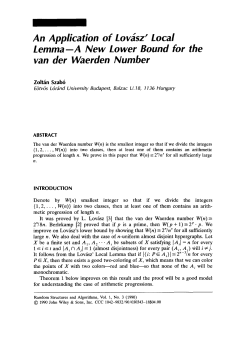
Figure 2 we report the results for the heteroscedastic case (µ = 1). The figure displays the (empirical)
rejection probability of the confidence intervals with nominal coverage of 95%. As before, ideally we
should see the empirical rejection probability of 5%. Again the top left figure reports the results for the
confidence intervals based on the naive post model selection estimator. Here too we see the striking lack
of robustness of this standard method; this occurs due to the direct equation (4.24) having coefficients ν0
that are not well separated from zero. We see from top right and bottom right and left plots of Figure 1,
that both of our proposed procedures perform substantially better, however, the optimal IV procedure
does not do as well as in the homoscedastic case. We also see from comparing the bottom left plot to other
plots that the confidence regions based on the post-double selection method significantly outperform the
optimal IV estimator, yielding empirical rejection frequencies close to the nominal level of 5%.
Thus, based on these experiments, we recommend to use the post-double selection procedure over the
optimal IV procedure.
4.2. Inference on Risk Factors in Childhood Malnutrition. The purpose of this section is to
examine practical usefulness of the new methods and contrast them with the standard post-selection
inference (that assumes that selection had worked perfectly).
We will assess statistical significance of socio-economic and biological factors on children’s malnutrition,
providing a methodological follow up on the previous studies done by [15] and [19]. The measure of
malnutrition is represented by the child’s height, which will be our response variable y. The socioeconomic and biological factors will be our regressors x, which we shall describe in more detail below. We
shall estimate the conditional first decile function of the child’s height given the factors (that is, we set
τ = .1). We’d like to perform inference on the size of the impact of the various factors on the conditional
decile of the child’s height. The problem has material significance, so it is important to conduct statistical
inference for this problem responsibly.
The data comes originally from the Demographic and Health Surveys (DHS) conducted regularly in
more than 75 countries; we employ the same selected sample of 37,649 as in Koenker (2012). All children
in the sample are between the ages of 0 and 5. The response variable y is the child’s height in centimeters.
The regressors x include child’s age, breast feeding in months, mothers body-mass index (BMI), mother’s
age, mother’s education, father’s education, number of living children in the family, and a large number
of categorical variables, with each category coded as binary (zero or one): child’s gender (male or female),
twin status (single or twin), the birth order (first, second, third, fourth, or fifth), the mother’s employment
status (employed or unemployed), mother’s religion (Hindu, Muslim, Christian, Sikh, or other), mother’s
ROBUST INFERENCE IN HIGH-DIMENSIONAL SPARSE QUANTILE REGRESSION MODELS
Naive Post Selection (C0.05,n) rp(0.05)
15
Optimal IV (C0.05,n) rp(0.05)
0.5
0.5
0.4
0.4
0.3
0.3
0.2
0.2
0.1
0.1
0
0
0.8
0.8
0.6
0.8
0.6
0.4
0.2
0.6
0.4
Ry2
Rd2
0.2
0
Rd2
0.8
0.6
0.4
0
0.4
0.2
Double Selection (C0.05,n) rp(0.05)
0.2
0
0
Ry2
Optimal IV (I0.05,n) rp(0.05)
0.5
0.5
0.4
0.4
0.3
0.3
0.2
0.2
0.1
0.1
0
0
0.8
0.8
0.6
0.6
0.4
0.2
Rd2
Figure 1.
0.8
0.8
0.6
0.6
0.4
0.4
Ry2
Rd2
0.2
0
0
0.4
0.2
0.2
0
0
Ry2
For the homoscedastic design (µ = 0), the figure displays the rejection probabilities of
the following confidence regions with nominal coverage of 95%: (a) the confidence region based upon
naive (single) selection procedure (top left panel), (b) the confidence region C0.05,n based the optimal
IV estimator based on (top right), (c) the confidence region, as defined in Algorithm 1′ , I0.05,n based
on the optimal IV procedure (bottom right panel), as defined in Algorithm 1′ , and (d) the confidence
region C0.05,n based on the post double selection estimator (bottom left panel), as defined in Algorithm
1′ . Each point in each of the plots corresponds to a different data-generating process indexed by pairs
of R2 values (R2d , R2y ) varying over the set {0, .1, . . . , .9} × {0, .1, . . . , .9}. The results are based on 500
replications for each of the 100 combinations of R2 ’s in each equation. The ideal rejection probability
should be 5%, so ideally we should be seeing a flat surface with height 5%.
residence (urban or rural), family’s wealth (poorest, poorer, middle, richer, richest), electricity (yes or
no), radio (yes or no), television (yes or no), bicycle (yes or no), motorcycle (yes or no), and car (yes or
no).
Although the number of covariates – 30 – is substantial, the sample size – 37,649– is much larger
than the number of covariates. Therefore, the dataset is very interesting from a methodological point of
view, since it gives us an opportunity to compare various methods for performing inference to an “ideal”
benchmark:
16
ROBUST INFERENCE IN HIGH-DIMENSIONAL SPARSE QUANTILE REGRESSION MODELS
Naive Post Selection (C0.05,n) rp(0.05)
Optimal IV (C0.05,n) rp(0.05)
0.5
0.5
0.4
0.4
0.3
0.3
0.2
0.2
0.1
0.1
0
0
0.8
0.8
0.6
0.8
0.6
0.4
0.2
0.6
0.4
Ry2
Rd2
0.2
0
Rd2
0.8
0.6
0.4
0
0.4
0.2
Double Selection (C0.05,n) rp(0.05)
0.2
0
0
Ry2
Optimal IV (I0.05,n) rp(0.05)
0.5
0.5
0.4
0.4
0.3
0.3
0.2
0.2
0.1
0.1
0
0
0.8
0.8
0.6
0.6
0.4
0.2
Rd2
Figure 2.
0.8
0.8
0.6
0.6
0.4
0.4
Ry2
Rd2
0.2
0
0
0.4
0.2
0.2
0
0
Ry2
For the heteroscedastic design (µ = 1), the figure displays the rejection probabilities of
the following confidence regions with nominal coverage of 95%: (a) the confidence region based upon
naive (single) selection procedure (top left panel), (b) the confidence region C0.05,n based the optimal
IV estimator based on (top right), (c) the confidence region, as defined in Algorithm 1′ , I0.05,n based
on the optimal IV procedure (bottom right panel), as defined in Algorithm 1′ , and (d) the confidence
region C0.05,n based on the post double selection estimator (bottom left panel), as defined in Algorithm
1′ . Each point in each of the plots corresponds to a different data-generating process indexed by pairs
of R2 values (R2d , R2y ) varying over the set {0, .1, . . . , .9} × {0, .1, . . . , .9}. The results are based on 500
replications for each of the 100 combinations of R2 ’s in each equation. The ideal rejection probability
should be 5%, so ideally we should be seeing a flat surface with height 5%.
(1) The “ideal” benchmark here is the standard inference based on the standard quantile regression
estimator without any model selection. Since the number of regressors p is much smaller than
the sample size n, this is a very good option. The latter was proven theoretically in [16] and in
[5] under the p → ∞, p3 /n → 0 regime. This is also the general option recommended by [20] and
[24] in the fixed p regime. Note that this “ideal” option does not apply in practice when p is
relatively large; however it certainly applies in the present example.
ROBUST INFERENCE IN HIGH-DIMENSIONAL SPARSE QUANTILE REGRESSION MODELS
17
(2) The standard post-selection inference method is the existing benchmark. This method performs
standard inference on the post-model selection estimator, “assuming” that the model selection
had worked perfectly. While this approach has some justification, we expect it to perform poorly,
based on our computational results and from theoretical results of [24]. In particular, it would
be very interesting to see if it gives misleading results as compared to the “ideal” option.
(3) We propose two methods, one based on the instrumental regression estimator (Algorithm 1) and
another based on double selection (Algorithm 2). The proposed methods do not assume perfect
selection, but rather builds a protection against (moderate) model selection mistakes. From the
theory we would expect the method to give results similar to the “ideal” option in (1).
We now will compare our proposal to the “ideal” benchmark and to the standard post-selection method.
We report the empirical results in Table 4.2. The first column reports results for the option 1, reporting
the estimates and standard errors enclosed in brackets. The second column reports results for option 2,
specifically the point estimates resulting from the use of ℓ1 -penalized quantile regression and the postpenalized quantile regression, reporting the standard errors as if there had been no model selection. The
third column and fourth column report the results for two versions – Algorithm 1 and Algorithm 2 – of
option 3. Each column reports point estimates, the standard errors, and the confidence region obtained
by inverting the robust Ln -statistic. Note that the Algorithms 1 and 2 are applied sequentially to each of
the variables. Similarly, in order to provide estimates and confidence intervals for all variables using the
naive approach, if a covariate was not selected by the ℓ1 -penalized quantile regression, it was included in
the post-model selection quantile regression for that variable.
What we see is very interesting. First of all, let us compare “ideal” option (column 1) and the naive
post-selection (column 2). Lasso selection method removes 16 out of 30 variables, many of which are
highly significant, as judged by the “ideal” option. (To judge significance we use normal approximations
and critical value of 3, which allows us to maintain 5% significance level after testing up to 50 hypotheses).
In particular, we see that the following highly significant variables were dropped by Lasso: mother’s BMI,
mother’s age, twin status, birth orders one and two, and indicator of the other religion. The standard
post-model selection inference then makes the assumption that these are true zeros, which lead us to
misleading conclusions about these effects. The standard post-model selection inference then proceeds
to judge the significance of other variables, in some cases deviating sharply and significantly from the
“ideal” benchmark. For example, there is a sharp disagreement on magnitudes of the impact of the birth
order variables and the wealth variables (for “richer” and “richest” categories). Overall, for the naive
post-selection, 8 out of 30 coefficients were more than 3 standard errors away from the coefficients of the
“ideal” option.
We now proceed to compare our proposed options to the “ideal” option. We see approximate agreement
in terms of magnitude, signs of coefficients, and in standard errors. In few instances, for example, for the
car ownership regressor, the disagreements in magnitude may appear large, but they become insignificant
once we account for the standard errors. In particular, the pointwise 95% confidence regions constructed
by inverting the Ln statistics all contain the estimates from the “ideal” option. Moreover, there is
18
ROBUST INFERENCE IN HIGH-DIMENSIONAL SPARSE QUANTILE REGRESSION MODELS
very little disagreement between Algorithms 1 (optimal IV) and Algorithm 2 (double selection). The
agreement here is good news from the point of view of our theory, since it confirms what we had expected
from our previous analysis. In particular, for the proposed methods, no coefficient estimate was more
than 1.5 standard errors away from the coefficient of the “ideal” option.
The main conclusion from our study is that the standard/naive post-selection inference can give misleading results, confirming our expectations and confirming predictions of [24]. Moreover, the proposed
inference procedures are able to deliver inference of high quality, which is very much in agreement with
the “ideal” benchmark.
5. Discussion
5.1. Variants of the Proposed Algorithms. There are several different ways to implement the sequence of steps underlying the two procedures outlined in Algorithms 1 and 2. The estimation of the
control function gτ can be done through other regularization methods like ℓ1 -qr instead of the post-ℓ1 qr estimator. The estimation of the instrument v in Step 2 can be carried out with Dantzig selector,
square-root Lasso or the associated post-model selection could be used instead of Lasso or Post-Lasso.
The instrumental quantile regression can be substituted by a 1-Step estimator from the ℓ1 -qr estimator
vi ].
bτ di + x′ βbτ )b
α
bτ of the form α̌τ = α
bτ + (En [b
v 2 ])−1 En [ϕτ (yi , α
i
i
Other variants can be constructed by using another valid instrument. An instrument ιi = ι(di , zi )
is valid if it satisfies Ē[fi ιi | zi ] = 0 and Ē[fi di ιi ] 6= 0. For example, a valid choice of instrument is
ιi = (di − E[di | zi ])/fi . Typically this choice of instruments does not lead to a semi-parametric efficient
estimator as the choices proposed in Algorithms 1 and 2 do. Nonetheless, the estimation of E[di | zi ] and
fi can be carried out separably which can lead to weaker regularity conditions.
5.2. Connection to Neymanization. In this section we make some connections to Neyman’s C(α)
test ([28, 29]). For the sake of exposition we assume that (yi , xi , di )ni=1 are i.i.d. and sparse models,
rmτ i = rgτ i = 0, i = 1, . . . , n. We consider the estimating equation for ατ :
E[ϕτ (yi , di ατ + x′i βτ )ιi ] = 0.
Our problem is to find useful instruments ιi such that
∂
E[ϕτ (yi , di ατ + x′i β)ιi ]|β=βτ = 0.
∂β
Under this property the estimator of ατ will be “immunized” against “crude” or nonregular estimation
of βτ , for example, via a post-selection procedure or some regularization procedure. Such immunization
ideas are in fact behind Neyman’s classical construction of his C(α) test, so we shall use the term
“Neymanization” to describe such procedure. There will be many instruments ιi that can achieve the
property stated above, and there will be one that is optimal.
The instruments can be constructed by taking ιi := vi /fi , where vi is the residual in the regression
equation:
wi di = wi mτ (zi ) + vi , E[wi vi |xi ] = 0,
(5.26)
ROBUST INFERENCE IN HIGH-DIMENSIONAL SPARSE QUANTILE REGRESSION MODELS
Table 1. Empirical Results
(1)
Variable
cage
mbmi
breastfeeding
mage
medu
edupartner
deadchildren
csexfemale
ctwintwin
cbirthorder2
cbirthorder3
cbirthorder4
cbirthorder5
munemployedemployed
mreligionhindu
mreligionmuslim
mreligionother
mreligionsikh
mresidencerural
wealthpoorer
wealthmiddle
wealthricher
wealthrichest
electricityyes
radioyes
televisionyes
refrigeratoryes
bicycleyes
motorcycleyes
caryes
(2)
(3)
qr
ℓ1 -qr
Naive
α̌τ
0.6456
(0.0030)
0.0603
(0.0159)
0.0691
(0.0036)
0.0684
(0.0090)
0.1590
(0.0136)
0.0175
(0.0125)
-0.0680
(0.1124)
-1.4625
(0.0948)
-1.7259
(0.3741)
-0.7256
(0.1073)
-1.2367
(0.1315)
-1.7455
(0.2244)
-2.4014
(0.1639)
0.0409
(0.1025)
-0.4351
(0.2232)
-0.3736
(0.2417)
-1.1448
(0.3296)
-0.5575
(0.2969)
0.1545
(0.0994)
0.2732
(0.1761)
0.8699
(0.1719)
1.3254
(0.2244)
2.0238
(0.2596)
0.3866
(0.1581)
-0.0385
(0.1218)
-0.1633
(0.1191)
0.1544
(0.1774)
0.1438
(0.1048)
0.6104
(0.1783)
0.2741
(0.2058)
0.6360
0.6458
(0.0027)
0.0663
(0.0139)
0.0689
(0.0038)
0.0454
(0.0147)
0.1870
(0.0145)
0.0460
(0.0148)
-0.2121
(0.0978)
-1.5084
(0.0897)
-1.8683
(0.2295)
-0.2230
(0.0983)
-0.5751
(0.1423)
-0.7910
(0.1938)
-1.1747
(0.1686)
0.0077
(0.1077)
-0.2423
(0.1080)
0.0294
(0.1438)
-0.6977
(0.3219)
0.3692
(0.1897)
0.1085
(0.1363)
-0.1946
(0.1231)
0.9197
(0.2236)
0.5754
(0.1408)
1.2967
(0.2263)
0.7555
(0.1398)
0.1363
(0.1214)
-0.0774
(0.1234)
0.2451
(0.2081)
0.1314
(0.1016)
0.5883
(0.1334)
0.5805
(0.2378)
0.6458
(0.0025)
0.0550
(0.0316)
0.0689
(0.0036)
0.0705
(0.0109)
0.1594
(0.0153)
0.0388
(0.0143)
-0.0791
(0.0653)
-1.5146
(0.0923)
-1.8683
(0.1880)
-0.7408
(0.1567)
-1.0737
(0.1556)
-1.7219
(0.2796)
-2.3700
(0.2574)
0.0342
(0.1055)
-0.5129
(0.2277)
-0.6177
(0.2629)
-1.2437
(0.3390)
-0.5437
(0.3653)
0.1519
(0.1313)
0.1187
(0.1505)
0.9113
(0.1784)
1.2751
( 0.1964)
1.9149
(0.2427)
0.4263
(0.1572)
0.0599
(0.1294)
-0.1112
(0.0971)
0.1907
(0.1716)
0.1791
(0.0853)
0.5214
(0.1702)
0.5544
(0.2610)
—
0.0538
—
0.2036
0.0147
—
-1.0786
—
—
—
-0.1892
-0.8459
—
—
—
—
—
—
-0.0183
—
0.3252
1.1167
0.3504
—
0.0122
0.0899
—
0.4823
—
Optimal IV
I0.05,n
[ 0.6400, 0.6514]
[ 0.0132, 0.0885]
[ 0.0577, 0.0762]
[ 0.0416, 0.0947]
[ 0.1246, 0.1870]
[ 0.0053, 0.0641]
[ -0.3522, 0.0394]
[ -1.7166, -1.3322]
[ -3.3481, -0.4652]
[ -1.0375, -0.3951]
[ -1.4627, -0.7821]
[ -2.2968, -1.2723]
[ -3.2407, -1.9384]
[ -0.2052, 0.2172]
[ -0.9171, -0.1523]
[ -1.1523, -0.1457]
[ -2.1037, -0.4828]
[ -1.5591, 0.4243]
[ -0.1295, 0.3875]
[ -0.1784, 0.5061]
[ 0.4698, 1.3149]
[ 0.7515, 1.5963]
[ 1.3086, 2.3893]
[ 0.1131, 0.7850]
[ -0.2100, 0.2682]
[ -0.3629, 0.0950]
[ -0.1642, 0.5086]
[ -0.0036, 0.3506]
[ 0.2471, 0.8125]
[ -0.0336, 1.0132]
Double Selection
α̌τ
0.6449
(0.0032)
0.0582
(0.0173)
0.0700
(0.0044)
0.0685
(0.0126)
0.1566
(0.0154)
0.0348
(0.0143)
-0.1546
(0.1121)
-1.5299
(0.1019)
-1.9248
(0.7375)
-0.6818
(0.1337)
-1.1326
(0.1719)
-1.5819
(0.2193)
-2.3041
(0.2564)
0.0379
(0.1124)
-0.5680
(0.1771)
-0.5119
(0.2176)
-1.1539
(0.3577)
-0.3408
(0.3889)
0.1678
(0.1311)
0.2648
(0.1877)
0.9173
(0.2158)
1.4040
(0.2505)
2.1133
(0.3318)
0.4582
(0.1577)
0.0640
(0.1207)
-0.0880
(0.1386)
0.2001
(0.1891)
0.1438
(0.1121)
0.5154
(0.1625)
0.5470
(0.2896)
19
20
ROBUST INFERENCE IN HIGH-DIMENSIONAL SPARSE QUANTILE REGRESSION MODELS
where wi is a nonnegative weight, a function of (di , zi ) only, for example wi = 1 or wi = fi – the latter
choice will in fact be optimal. Note that function mτ (zi ) solves the least squares problem
min E {wi di − wi h(zi )}2 ,
h∈H
(5.27)
where H is the class of measurable functions h(zi ) such that E[wi2 h2 (zi )] < ∞. Our assumption is that
the mτ (zi ) is a sparse function x′i θτ , with kθτ k0 6 s so that
wi di = wi x′i θτ + vi , E[wi vi |xi ] = 0.
(5.28)
In finite samples, the sparsity assumption allows to employ post-Lasso and Lasso to solve the least squares
problem above approximately, and estimate ιi . Of course, the use of other structured assumptions may
motivate the use of other regularization methods.
√
Arguments similar to those in the proofs show that, for n(α − ατ ) = O(1),
√
n{En [ϕτ (yi , di α + x′i βbτ )vi ] − En [ϕτ (yi , di α − x′i βτ )ιi ]} = oP (1),
for βbτ based on a sparse estimation procedure, despite the fact that βbτ converges to βτ at a slower rate
√
than 1/ n. That is, the empirical estimating equations behave as if βτ is known. Hence for estimation
we can use α̌τ as a minimizer of the statistic:
√
′b
2
Ln (α) = c−1
n | nEn [ϕτ (yi , di α − xi βτ )ιi ]| ,
χ2 (1), we can also use the statistic directly for
where cn = En [ϕ2τ (yi , di α − x′i βbτ )ι2i ]. Since Ln (ατ )
testing hypotheses and for construction of confidence sets.
This is in fact a version of Neyman’s C(α) test statistic, adapted to the present non-smooth setting. The usual expression of C(α) statistic is different. To see a more familiar form, note that
θτ = Ē[wi2 xi x′i ]− Ē[wi2 di x′i ], where A− denotes a generalized inverse of A, and write
so that,
bi := ϕτ (yi , di α + x′i βbτ ),
ιi = (wi /fi )di − (wi /fi )x′i Ē[wi2 xi x′i ]− Ē[wi2 di x′i ], and ϕ
√
Ln (α) = c−1
bi (wi /fi )di ] − En [ϕ
bi (wi /fi )xi ]′ Ē[wi2 xi x′i ]− Ē[wi2 di x′i ]}|2 .
n | n{En [ϕ
This is indeed a familiar form of a C(α) statistic.
The estimator α̌τ that minimizes Ln up to oP (1), under suitable regularity conditions,
√
N (0, 1), σn2 = τ (1 − τ )E[fi di vi ]−2 E[vi2 ].
σn−1 n(α̌τ − ατ )
It is easy to show that the smallest value of σn2 is achieved by using ιi = ι∗i induced by setting wi = fi :
σn∗2 = τ (1 − τ )E[vi∗2 ]−1 .
(5.29)
Thus, setting wi = fi gives an optimal instrument amongst all “immunizing” instruments generated by
the process described above. Obviously, this improvement translates into shorter confidence intervals and
better testing based on either α̌τ or Ln . While wi = fi is optimal, fi will have to be estimated in practice,
resulting actually in more stringent condition than when using non-optimal, known weights, e.g., wi = 1.
The use of known weights may also give better behavior under misspecification of the model. Under
homoscedasticity, wi = 1 is an optimal weight.
ROBUST INFERENCE IN HIGH-DIMENSIONAL SPARSE QUANTILE REGRESSION MODELS
21
5.3. Minimax Efficiency. There is also a clean connection to the (local) minimax efficiency analysis
from the semiparametric efficiency analysis. [23] derives an efficient score function for the partially linear
median regression model:
Si = 2ϕτ (yi , di ατ + x′i βτ )fi [di − m∗τ (z)],
where m∗τ (zi ) is mτ (zi ) in (5.26) induced by the weight wi = fi :
m∗τ (zi ) =
E[fi2 di |zi ]
.
E[fi2 |zi ]
Using the assumption m∗τ (zi ) = x′i θτ∗ , where kθτ∗ k0 6 s ≪ n is sparse, we have that
Si = 2ϕτ (yi , di ατ + x′i βτ )vi∗ ,
which is the score that was constructed using Neymanization. It follows that the estimator based on the
instrument vi∗ is actually efficient in the minimax sense (see Theorem 18.4 in [21]), and inference about
ατ based on this estimator provides best minimax power against local alternatives (see Theorem 18.12
in [21]).
The claim above is formal as long as, given a law Qn , the least favorable submodels are permitted as
deviations that lie within the overall model. Specifically, given a law Qn , we shall need to allow for a
certain neighborhood Qδn of Qn such that Qn ∈ Qδn ⊂ Qn , where the overall model Qn is defined similarly
as before, except now permitting heteroscedasticity (or we can keep homoscedasticity fi = fǫ to maintain
formality). To allow for this we consider a collection of models indexed by a parameter t = (t1 , t2 ):
yi
fi di
=
di (ατ + t1 ) + x′i (βτ + t2 θτ∗ ) + ǫi ,
=
fi x′i θτ∗
+
vi∗ ,
E[fi vi∗ |xi ]
ktk 6 δ,
= 0,
(5.30)
(5.31)
where kβτ k0 ∨ kθτ∗ k0 6 s/2 and conditions as in Section 2 hold. The case with t = 0 generates the model
Qn ; by varying t within δ-ball, we generate models Qδn , containing the least favorable deviations. By
[23], the efficient score for the model given above is Si , so we cannot have a better regular estimator than
the estimator whose influence function is J −1 Si , where J = E[Si2 ]. Since our model Qn contains Qδn ,
all the formal conclusions about (local minimax) optimality of our estimators hold from theorems cited
above (using subsequence arguments to handle models changing with n). Our estimators are regular,
√
since under Qtn with t = (O(1/ n), o(1)), their first order asymptotics do not change, as a consequence
of Theorems in Section 2. (Though our theorems actually prove more than this.)
Acknowledgements
We would like to specially thank Roger Koenker for providing the data for the empirical example
and for many insightful discussions on inference. We would also like to thank the participants of the
December 2012 Luminy conference on Nonparametric and high-dimensional statistics, the November
2012 Oberwolfach workshop on Frontiers in Quantile Regression, the August 2012 8th World Congress
in Probability and Statistics, and a seminar at the University of Michigan.
22
ROBUST INFERENCE IN HIGH-DIMENSIONAL SPARSE QUANTILE REGRESSION MODELS
Appendix A. Analysis under High-Level Conditions
This section contains the main tools used in establishing the main inferential results. The highlevel conditions here are intended to be applicable in a variety of settings and they are implied by the
regularities conditions provided in the previous sections. The results provided here are of independent
interest (e.g. properties of Lasso under estimated weights). We establish the inferential results (2.16) and
(2.19) in Section A.3 under high level conditions. To verify these high-level conditions we need rates of
convergence for the estimated instruments b
v and the estimated confounding function b
gτ (z) = x′ βbτ which
are established in sections A.2 and A.1 respectively. The main design condition relies on the restricted
eigenvalue proposed in [11], namely for x̃i = [di , x′i ]′
κc =
inf
kδT c k1 6ckδT k1
kx̃′i δk2,n /kδT k
(A.32)
where c = (c + 1)/(c − 1) for the slack constant c > 1, see [11]. It is well known that Condition SE implies
that κc is bounded away from zero if c is bounded, see [11].
A.1. ℓ1 -Penalized Quantile Regression. In this section for a quantile index u ∈ (0, 1), we consider
the equation
ỹi = x̃′i ηu + rui + ǫi , u-quantile of (ǫi | x̃i , rui ) = 0
(A.33)
where we observe {(ỹi , x̃i ) : i = 1, . . . , n}, which are independent across i. To estimate ηu we consider
the ℓ1 -penalized u-quantile regression estimate
ηbu ∈ arg min En [ρu (ỹi − x̃′i η)] +
η
λ
kηk1
n
and the associated post-model selection estimate
ηeu ∈ arg min { En [ρu (ỹi − x̃′i η)] : ηj = 0 if ηbuj = 0} .
η
(A.34)
As established in [3] for sparse models and in [17] for approximately sparse models, under the event
that
λ
> ckEn [(u − 1{ỹi 6 x̃′i ηu + rui })x̃i ]k∞
(A.35)
n
the estimator above achieves good theoretical guarantees under mild design conditions. Although ηu is
unknown, we can set λ so that the event in (A.35) holds with high probability. In particular, the pivotal
rule proposed in [3] and generalized in [17] proposes to set λ := cnΛ(1 − γ | x̃) for c > 1 where
Λ(1 − γ | x̃) = (1 − γ) − quantile of kEn [(u − 1{Ui 6 u})x̃i ]k∞
(A.36)
where Ui ∼ U (0, 1) are independent random variables conditional on x̃i , i = 1, . . . , n. This quantity can
be easily approximated via simulations. Below we summarize the high level conditions we require.
Condition PQR. Let Tu = support(ηu ) and normalize En [x̃2ij ] = 1, j = 1, . . . , p. Assume that
p
for some s > 1, kηu k0 6 s, krui k2,n 6 C s/n. Further, the conditional distribution function of ǫi
is absolutely continuous with continuously differentiable density fǫ (· | di , zi ) such that 0 < f 6 fi 6
supǫ fǫi |di ,zi (ǫ | di , zi ) 6 f¯, supǫ fǫ′i |di ,zi (ǫ | di , zi ) < f¯′ for fixed constants f , f¯ and f¯′ .
ROBUST INFERENCE IN HIGH-DIMENSIONAL SPARSE QUANTILE REGRESSION MODELS
23
Condition PQR is implied by Condition AS. The conditions on the approximation error and near
orthogonality conditions follows from choosing a model ηu that optimally balance the bias/variance
trade-off. The assumption on the conditional density is standard in the quantile regression literature
even with fixed p case developed in [20] or the case of p increasing slower than n studied in [5].
Next we present bounds on the prediction norm of the ℓ1 -penalized quantile regression estimator.
Lemma 1. Under Condition PQR, setting λ > cnΛ(1 − γ | x̃), we have with probability 1 − 4γ for n
large enough
kx̃′i (b
ηu
− ηu )k2,n
r
√
1
λ s
s log(p/γ)
+
. N :=
nκ2c
κ2c
n
provided that for Au := ∆2c ∪ {v : kx̃′i vk2,n = N, kvk1 6 8Ccs log(p/γ)/λ}, we have
sup
δ̄∈Au
En [|rui ||x̃′i δ̄|2 ]
En [|x̃′i δ̄|3 ]
+ N sup
→ 0.
′
′ 2 3/2
2
En [|x̃i δ̄| ]
δ̄∈Au En [|x̃i δ̄| ]
Lemma 1 establishes the rate of convergence in the prediction norm for the ℓ1 -qr estimator. Exact constants are derived in the proof. The extra growth condition required for identification is mild. For instance
p
we typically have λ ∼ log(n ∨ p)/n and for many designs of interest we have inf δ∈∆c kx̃′i δk32,n /En [|x̃′i δ|3 ]
bounded away from zero (see [3]). For more general designs we have
inf
δ∈Au
kx̃′i δk32,n
kx̃′i δk2,n
κ2c
λN
>
inf
> √
∧
.
′
En [|x̃i δ|3 ] δ∈Au kδk1 maxi6n kx̃i k∞
s(1 + c) maxi6n kx̃i k∞ 8Ccs log(p/γ) maxi6n kx̃i k∞
Lemma 2 (Estimation Error of Post-ℓ1-qr). Assume Condition PQR holds, and that the Post-ℓ1 -qr is
b > En [ρu (ỹi − x̃′ ηbu )] −
based on an arbitrary vector ηbu . Let r̄u > krui k2,n , sbu > |support(b
ηu )| and Q
i
En [ρu (ỹi − x̃′i ηu ))] hold with probability 1 − γ. Then we have for n large enough, with probability 1 − γ −
ǫ − o(1)
kx̃′i (e
ηu
provided that
e :=
− ηu )k2,n . N
s
(b
su + s) log(p/ε)
b 1/2
+ f¯r̄u + Q
nφmin (b
su + s)
En [|x̃′i δ̄|3 ]
En [|rui ||x̃′i δ̄|2 ]
e
+
N
sup
→ 0.
′ 2 3/2
En [|x̃′i δ̄|2 ]
kδ̄k0 6b
su +s En [|x̃i δ̄| ]
kδ̄k0 6b
su +s
sup
Lemma 2 provides the rate of convergence in the prediction norm for the post model selection estimator
despite of possible imperfect model selection. In the current nonparametric setting it is unlikely for the
coefficients to exhibit a large separation from zero. The rates rely on the overall quality of the selected
model by ℓ1 -penalized quantile regression and the overall number of components sbu . Once again the extra
growth condition required for identification is mild. For more general designs we have
p
kx̃′i δk32,n
φmin (b
su + s)
kx̃′i δk2,n
>
inf
>√
.
inf
′
3
kδk0 6b
su +s kδk1 maxi6n kx̃i k∞
kδk0 6b
su +s En [|x̃i δ| ]
sbu + s maxi6n kx̃i k∞
24
ROBUST INFERENCE IN HIGH-DIMENSIONAL SPARSE QUANTILE REGRESSION MODELS
A.2. Lasso with Estimated Weights. In this section we consider the equation
fi di = fi mτ (zi ) + vi = fi x′i θτ + fi rmτ i + vi , E[fi vi | zi ] = 0
(A.37)
where we observe {(di , zi , xi = P (zi )) : i = 1, . . . , n}, which are independent across i. We do not observe
{fi = fτ (di , zi )}n directly, but we assume that estimates {fbi }n are available. Also, we have that
i=1
i=1
Tmτ = support(θτ ) is unknown but a sparsity condition holds, namely |Tmτ | 6 s. To estimate θmτ and
vi , we compute
λ b
bi = fbi (di − x′i θbτ ), i = 1, . . . , n,
(A.38)
θbτ ∈ arg min En [fbi2 (di − x′i θ)2 ] + kΓ
τ θk1 and set v
θ
n
b τ are the associated penalty level and loadings specified below. The new difficulty is to
where λ and Γ
account for the impact of estimated weights fbi . Although this impact on the estimation of θτ is minor,
the estimated weights impact estimates of vi can be more substantial.
We will establish bounds on the penalty parameter λ so that with high probability the following
regularization event occurs
λ
b −1
> 2ckΓ
(A.39)
τ En [fi xi vi ]k∞ .
n
c k1 6
As discussed in [11, 4, 8], the event above allows to exploit the restricted set condition kθbτ Tmτ
b
b
c̃kθτ Tmτ − θτ k1 for some c̃ > 1. Thus rates of convergence for θτ and vbi defined on (A.38) can be
established based on the restricted eigenvalue κc̃ defined in (A.32) with x̃i = xi .
However, the estimation error in the estimate fbi of fi could slow the rates of convergence. The following
are sufficient high-level conditions.
Condition WL. For the model (A.37), normalize En [x2ij ] = 1, j = 1, . . . , p, and suppose that:
2
−1
(i) for s > 1 we have kθτ k0 6 s, En [rmτ
(1 − γ/2p) 6 δn n1/3 ,
i ] 6 Cs/n, Φ
{Ē[|f xij vi |3 ]}1/3
6 C,
(ii) 0 < f 6 fi 6 f¯ uniformly in n, and 0 < c 6 E[vi2 | xi ] 6 c̄ < ∞, a.s., max {Ē[|fii xij
vi |2 ]}1/2
j6p
(iii) with probability 1 − ∆n we have maxi6n kxi k∞ 6 Kx ,
2
2
max|(En − Ē)[fi2 x2ij vi2 ]| 6 δn , max En [(fbi − fi )2 x2ij vi2 ] 6 δn , En [fbi2 rmτ
i ] 6 cr , En
j6p
j6p
h
(fbi2 −fi2 )2 2
vi
fi2
i
6 c2f .
bτ 0 6 Γ
b τ 6 uΓ
b τ 0 , where Γ
b τ 0jj = {En [fb2 x2 v 2 ]}1/2 , 1 − δn 6 ℓ 6 u 6 C with probability 1 − ∆n .
(iv) ℓΓ
i ij i
Comment A.1. Condition WL(i) is a standard condition on the approximation error that yields the
optimal bias variance trade-off (see [4]) and imposes a growth restriction on p relative to n, in particular
log p = o(n1/3 ). Condition WL(ii) imposes conditions on the conditional density function and mild
moment conditions which are standard in quantile regression models even with fixed dimensions, see [20].
Condition WL(iii) requires high-level rates of convergence for the estimate fbi . Several primitive moment
conditions imply first requirement in Condition WL(iii). These conditions allow the use of self-normalized
moderate deviation theory to control heteroscedastic non-Gaussian errors similarly to [2] where there are
no estimated weights. Condition WL(iv) corresponds to the asymptotically valid penalty loading in [2]
b τ in (2.11).
which is satisfied by the proposed choice Γ
Next we present results on the performance of the estimators generated by Lasso with estimated
weights.
ROBUST INFERENCE IN HIGH-DIMENSIONAL SPARSE QUANTILE REGRESSION MODELS
25
√
Lemma 3 (Rates of Convergence for Lasso). Under Condition WL and setting λ > 2c′ nΦ−1 (1 − γ/2p)
for c′ > c > 1, we have for n large enough with probability 1 − γ − o(1)
√ λ s
1
kfbi x′i (θbτ − θτ )k2,n 6 2{cf + cr } +
u+
nb
κc̃
c
√
b −1 k∞ n
1 2ckΓ
1
λs
s{c
+
c
}
f
r
τ0
b
+ 1+
u+
+
{cf + cr }2
k θτ − θτ k 1 6 2
b2c̃
κ2c̃
b
nb
κc̃ κ
c
2c̃
ℓc − 1 λ
b −1 k∞ kΓ
b τ 0 k∞ (uc + 1)/(ℓc − 1)
where c̃ = kΓ
τ0
Lemma 3 above establishes the rate of convergence for Lasso with estimated weights. This automati-
cally leads to bounds on the estimated instrument vbi obtained with Lasso through the identity
vi
vi − vi = (fbi − fi ) + fbi x′i (θτ − θbτ ) + fbi rmτ i .
b
fi
(A.40)
The Post-Lasso estimator applies the least squares estimator to the model selected by the Lasso estimator
(A.38),
n
o
En [fbi2 (di − x′i θ)2 ] : θj = 0, if θbτ j = 0 , set ṽi = fbi (di − x′i θeτ ).
θeτ ∈ arg minp
θ∈R
It aims to remove the bias towards zero induced by the ℓ1 -penalty function which is used to select
components. Sparsity properties of the Lasso estimator θbτ under estimated weights follows similarly to
the standard Lasso analysis derived in [2]. By combining such sparsity properties and the rates in the
prediction norm we can establish rates for the post-model selection estimator under estimated weights.
The following result summarizes the properties of the Post-Lasso estimator.
Lemma 4 (Model Selection Properties of Lasso and Properties of Post-Lasso). Suppose that Condition
2
2
WL holds, and κ′ 6 φmin ({s + nλ2 {c2f + c2r }}/δn) 6 φmax ({s + nλ2 {c2f + c2r }}/δn ) 6 κ′′ for some positive
and bounded constants κ′ , κ′′ . Then the data-dependent model Tbmτ selected by the Lasso estimator with
√
λ > 2c′ nΦ−1 (1 − γ/2p) for c′ > c > 1, satisfies with probability 1 − γ − o(1):
kθeτ k0 = |Tbmτ | . s +
Moreover, the corresponding Post-Lasso estimator obeys
s
kx′i (θeτ − θτ )k2,n .P cf + cr +
n2 2
{c + c2r }
λ2 f
(A.41)
√
|Tbmτ | log(p ∨ n) λ s
.
+
n
nκc
A.3. Instrumental Quantile Regression with Estimated Data. Next we turn to analyze the instrumental quantile regression discussed in Section 2. Condition IQR below suffices to make the impact
of the estimation of instruments negligible to the first order asymptotics of the estimator α̌τ . Primitive
conditions that imply Condition IQR are provided and discussed in the main text.
Let (d, z) ∈ D × Z. In this section for h̃ = (g̃, ι̃), where g̃ is a function of variable z, and the instrument
ι̃ is a function that maps (d, x) 7→ ι̃(d, z) we write
ψα̃,h̃ (yi , di , zi ) = ψα̃,g̃,ι̃ (yi , di , zi ) = (τ − 1{yi 6 g̃(zi ) + di α})ι̃(di , zi ) = (τ − 1{yi 6 g̃i + di α})ι̃i .
We assume that the estimated functions gb and b
ι satisfy the following condition.
26
ROBUST INFERENCE IN HIGH-DIMENSIONAL SPARSE QUANTILE REGRESSION MODELS
Condition IQR. F or some sequences δn → 0 and ∆n → 0 with probability at least 1 − ∆n :
(i) fyi |di ,zi (y | di , zi ) 6 f¯, fy′ i |di ,zi (y | di , zi ) 6 f¯′ ; Ē[fi ι0i | zi ] = 0, 0 < c 6 |Ē[fi di ι0i ]|, and
maxi6n {E[ι40i ]}1/2 ∨ {E[d4i ]}1/2 6 C;
(ii) {α : |α − ατ | 6 n−1/2 /δn } ⊂ Aτ , where Aτ is a (possibly random) compact interval;
(iii) the estimated quantities b
h = (b
g, b
ι) satisfy
max{1 + |ι0i | + |b
ιi − ι0i |}1/2 kgτ i − gbi k2,n 6 δn n−1/4 ,
i6n
|En [fi ι0i {b
gi − gτ i }]| 6 δn n−1/2
kb
ιi − ι0i k2,n 6 δn , kgτ i − gbi k2,n · kb
ιi − ι0i k2,n 6 δn n−1/2 ,
i
h
sup (En − Ē) ψα,bh (yi , di , zi ) − ψα,h0 (yi , di , zi ) 6 δn n−1/2
(A.42)
(A.43)
α∈Aτ
|α̌τ − ατ | 6 δn
and
En [ψα̌τ ,bh (yi , di , zi )]| 6 δn n−1/2
(A.44)
(iv) kb
ιi − ι0i k2,n 6 δn and k1{|ǫi | 6 |di (ατ − α̌τ ) + gτ i − gbi |}k2,n 6 δn2 .
Lemma 5. Under Condition IQR(i,ii,iii) we have
√
{Ē[fi di ι0i ]−1 Ē[τ (1 − τ )ι20i ]Ē[fi di ι0i ]−1 }−1/2 n(α̌τ − ατ )
N (0, 1).
Moreover, if additionally IQR(iv) holds we have
χ2 (1)
nLn (ατ )
and the variance estimator is consistent, namely
En [fbi dib
ιi ]−1 En [(τ − 1{yi 6 gbi + di α̌τ })2b
ι2i ]En [fbi dib
ιi ]−1 →P Ē[fi di ι0i ]−1 Ē[τ (1 − τ )ι20i ]Ē[fi di ι0i ]−1 .
Appendix B. Results for Section 3
Proof of Theorem 1. We will verify Condition IQR and the result follows by Lemma 5. Condition IQR(i)
is assumed.
Condition SE implies that κc is bounded away from zero for n sufficiently large. Step 1 relies on
Post-ℓ1-qr. By the truncation we have sbτ = kβeτ k0 6 Cs for any C > 2. Thus, by Condition SE
φmin (b
sτ + s) is bounded away from zero since sbτ + s 6 ℓn s for large enough n with probability 1 − ∆n .
(2s)
Moreover, Condition PQR is implied by Condition AS. Lemma 6 ensures that kβbτ −βτ k1 6 2kβbτ −βτ k1
p
(2s)
and kx̃′i (βbτ − βτ )k2,n 6 kx̃′i (βbτ − βτ )k2,n + φmax (s)/skβbτ − βτ k1 since φmax (k)/k is decreasing in
p
s log(n ∨ p)/n provided the side conditions
k. Therefore, by Lemma 2 we have kx′i (βeτ − βτ )k2,n .P
required in Lemmas 1 and 2. To verify those side conditions for Lemma 2 let x̃i = (di , x′i )′ and δ = (δd , δx′ )′ .
By Condition SE and En [|di |3 ] .P Ē[|di |3 ] 6 C, we have
kx̃′i δk32,n
′ 3
E
kδk0 6s+Cs n [|x̃i δ| ]
inf
>
>
{φmin (s+Cs)}3/2 kδk3
inf
′
3
3
3
kδk0 6s+Cs 4En [|xi δx | ]+4|δd | En [|di | ]
3/2
{φmin (s+Cs)}
kδk3
inf
2
3
3
4K
x kδx k1 φmax (s+Cs)kδx k +4kδk En [|di | ]
kδk 6s+Cs
0
{φmin (s+Cs)}3/2
√
s+Csφmax (s+Cs)+4En [|di |3 ]
&P Kx1√s .
p
The relation above and the conditions Kx2 s2 log2 (p ∨ n) 6 δn n and λ . n log(p ∨ n) yields
√
√
kx̃′i δk32,n
n φmin (s+Cs)
n
inf
&P Kx s log(p∨n)
→ ∞.
√ √
En [|x̃′ δ|3 ]
>
λ s+
4Kx
sn log(p∨n) kδk0 6s+Cs
i
ROBUST INFERENCE IN HIGH-DIMENSIONAL SPARSE QUANTILE REGRESSION MODELS
27
Moreover, noting that kδx k ∨ |δd | 6 kδk, we have
sup
kδk0 6s+Cs
En [|rgτ i | |x̃′i δ|2 ]
kx̃′i δk22,n
62
sup
kδk0 6s+Cs
62
sup
En [|rgτ i | |x′i δx |2 ]+En [|rgτ i |d2i δd2 ]
φmin (s+Cs)kδk2
krgτ i k2,n
kδk0 6s+Cs
p s Kx √s+Cs
n φmin (s+Cs)
6C
√
φmax (s+Cs)kδx kKx kδx k1
φmin (s+Cs)kδx k2
+
krgτ i k2,n kd2i k2,n
φmin (s+Cs)
→ 0.
The verification of the side condition for Lemma 1 follows similarly.
Step 2 relies on Post-Lasso. Condition WL(i) and (ii) are implied by Conditions AS. Indeed, the
moment conditions in AS imply the first part, the second part Φ−1 (1 − γ/2p) 6 δn n1/3 is implied by
log(1/γ) . log(p ∨ n) and log3 p 6 δn n. Next we establish Condition WL(iii) under known conditional
density. The first condition is implied by Lemma 8 under the moment conditions and the growth condition
Kx4 log p 6 δn n and fi 6 f¯. Since fbi = fi the other requirements in WL(iii) follows.
Next we establish Condition WL(iv). Note that
maxj6p |En [x2ij (fi di )2 ] − Ē[x2ij (fi di )2 ]| 6 maxj6p |(En − Ē)[x2ij (fi di )2 ]| .P δn
and
maxj6p |En [fi2 x2ij vi2 ] − Ē[fi2 x2ij vi2 ]| 6 maxj6p |(En − Ē)[fi2 x2ij vi2 ]| .P δn
b τ 0jj is bounded away
by Lemma 8 because Ē[fi2 x2ij vi2 ] is bounded away from zero and from above. Thus Γ
from zero and from above with probability 1 − o(1). Next note that
4
(maxi6n fi2 )Ē[x2ij (fi di )2 ] 6 f maxj6p Ē[x2ij d2i ] 6 C, and
(maxi6n fi2 )Ē[x2ij (fi di )2 ] = (maxi6n fi2 )Ē[x2ij (vi2 + 2mτ i (zi )fi vi + fi2 m2τ i (zi ))]
= (maxi6n fi2 )Ē[x2ij vi2 ] + (maxi6n fi2 )Ē[x2ij fi2 m2τ i (zi )] > Ē[fi2 x2ij vi2 ].
Therefore, the initial penalty loadings {(maxi6n fi2 )En [x2ij (fi di )2 ]}j=1,...,p satisfy Condition WL(iv) with
b τ jj using vbi
ℓ → 1 and u 6 C. By Lemma 4 and the growth conditions we have that the penalty loadings Γ
p
′ e
b
b
b
also satisfy Γτ 0jj − δn 6 Γτ jj 6 uΓτ 0jj . Thus, by Lemma 4 we have kxi (θτ − θτ )k2,n .P s log(n ∨ p)/n
and kθeτ k0 .P s.
Step 3 relies on instrumental quantile regression. Condition IQR(iii) relation (A.42) follows by the
rates for βeτ and θeτ and the growth condition Kx2 s2 log2 (p ∨ n) 6 δn n.
To show Condition IQR(iii) relation (A.43) we will consider the class of functions
p
F = {1{yi 6 x′i β + di α} − 1{yi 6 x′i βτ + di α} : kβk0 6 Cs, kβ − βτ k 6 C s log(p ∨ n)/n}.
p
Since F is the union of Cs
VC classes of dimension Cs, it satisfies log N (εkF k2,Pn , F , Pn ) . Cs log(p ∨
n) + Cs log(1/ε).
Note that
i
h
vi − ϕτ (yi , gτ i + di α)vi sup (En − Ē) ϕτ (yi , x′i βeτ + di α)b
α∈Aτ
i
h
vi − vi } +
6 sup (En − Ē) ϕτ (yi , x′i βeτ + di α){b
(B.45)
α∈Aτ
i
h
+ sup (En − Ē) {ϕτ (yi , x′i βeτ + di α) − ϕτ (yi , x′i βτ + di α)}vi +
α∈Aτ
(B.46)
28
ROBUST INFERENCE IN HIGH-DIMENSIONAL SPARSE QUANTILE REGRESSION MODELS
+ sup (En − Ē) [{ϕτ (yi , x′i βτ + di α) − ϕτ (yi , gτ i + di α)}vi ] .
(B.47)
α∈Aτ
To bound (B.45), we write vbi − vi = fi x′i {θeτ − θτ } + fi rmτ i . Substitute the equation above into (B.45).
Using triangle inequality and Lemma 9 together with the entropy bounds for F and
p
G = {δ : kx′i δk2,n 6 C s log(p ∨ n)/n, kδk0 6 Cs},
we have
r
r
h
i
Cs log(p ∨ n) s log(p ∨ n)
′e
′ e
(B.45).(i) = sup (En − Ē) ϕτ (yi , xi βτ + di α)fi xi {θτ − θτ } .P
n
n
α∈Aτ
r
r
h
i
Cs log(p ∨ n) s
(B.45).(ii) = sup (En − Ē) ϕτ (yi , x′i βeτ + di α)fi rmτ i .P
n
n
α∈Aτ
p
To bound (B.46), by Lemma 10, kx′i {βeτ −βτ }k2,n .P s log(p ∨ n)/n, Ē[(1{yi 6 a}−1{yi 6 b})2 vi2 ] 6
Ē[f¯vi2 |a − b|], and kvi2 k2,n .P {Ē[vi4 ]}1/2 , we have
i
h
sup (En − Ē) {ϕτ (yi , x′i βeτ + di α) − ϕτ (yi , x′i βτ + di α)}vi α∈Aτ
.P
r
Cs log(p ∨ n) log n
n
!1/2
r
r
Cs
log(p
∨
n)
s
log(p
∨
n)
{Ē[vi4 ]}1/2 f¯
= oP (n−1/2 )
+
{Ē[vi4 ]}1/2
n
n
provided that s3 log3 (p ∨ n) log2 n 6 δn n. Similarly, to bound (B.47), by Lemma 10 and krgτ i k2,n .P
p
s/n, we have
sup (En − Ē) [{ϕτ (yi , x′i βτ + di α) − ϕτ (yi , gτ i + di α)}vi ]
α∈Aτ
.P
r
log n
n
1/2
{Ē[vi4 ]}1/2 f¯krgτ i k2,n
+
{Ē[vi4 ]}1/2
r
log n
n
!1/2
= oP (n−1/2 ).
Next we verify the second part of Condition IQR(iii) relation (A.44). To show
|En [ϕτ (yi , x′i βeτ + di α̌τ )b
vi ]| .P δn n−1/2
consider that
Ln (α̌τ ) =
6
vi ]}2
{En [ϕτ (yi , x′i βeτ + di α)b
vi ]}2
{En [ϕτ (yi , x′i βeτ + di α̌τ )b
= min
e
α∈Aτ E [ϕ2 (y , x′ β
vi2 ]
vi2 ]
En [ϕ2τ (yi , x′i βeτ + di α̌τ )b
n τ i
i τ + di α)b
1
vi ]}2
min {En [ϕτ (yi , x′i βeτ + di α)b
τ 2 (1 − τ )2 En [b
vi2 ] α∈Aτ
Letting ϕ
bi (α) = ϕτ (yi , x′i βeτ + di α), ϕi (α) = ϕτ (yi , gτ i + di α) we have
|En [ϕ
bi (α)b
vi ]| 6 |(En − Ē)[ϕ
bi (α)b
vi − ϕi (α)vi ]| + |Ē[ϕ
bi (α)b
vi ] − Ē[ϕi (α)vi ]| + |En [ϕi (α)vi ]|
.P δn n−1/2 + δn |α − ατ | + |En [ϕi (α)vi ]|
where the bias term |Ē[ϕ
bi (α)b
vi ] − Ē[ϕi (α)vi ]| .P δn n−1/2 + δn |α − ατ | follows from relations (H.74),
(H.75), and (H.77) in the Supplementary Appendix. Therefore,
ROBUST INFERENCE IN HIGH-DIMENSIONAL SPARSE QUANTILE REGRESSION MODELS
29
{En [b
v 2 ]}−1
{ En [ϕ
bi (α̌τ )b
vi ] }2
6 Ln (α̌τ ) 6 2 i 2 min { En [ϕ
bi (α)b
vi ] }2
2
En [b
vi ]
τ (1 − τ ) α∈Aτ
{En [b
v 2 ]}−1
min
{ δn n−1/2 + δn |α − ατ | + |En [ϕi (α)vi ]| }2
.P 2 i 2
τ (1 − τ ) α∈{α:|α−ατ |6n−1/2 /δn }
{En [b
v 2 ]}−1
.P 2 i 2 { δn n−1/2 + δn |α∗ − ατ | + |En [ϕi (α∗ )vi ]| }2
τ (1 − τ )
where α∗ ∈ arg minα∈{α:|α−ατ |6n−1/2 /δn } |En [ϕi (α)vi ]|. It follows that |α∗ −ατ | .P n−1/2 and |En [ϕi (α∗ )vi ]| .P
n−1 maxi6n |vi |. Therefore, since maxi6n |vi | .P n1/4 by Ē[vi4 ] 6 C, we have
|En [ϕ
bi (α̌τ )b
vi ]| .P
δn n−1/2
.
τ (1 − τ )
Proof of Theorem 2. The analysis of Step 1 and 2 are identical to the corresponding analysis in the proof
of Theorem 1. Define (ỹi ; x̃i ) = (fi yi ; fi di , fi xi ), since fi = f (di , xi ) and 0 < f 6 fi 6 f¯, by Lemma 2
p
we have kx′i β̌τ − gτ i k2,n .P s log(p ∨ n)/n and |α̌τ − ατ | 6 δn . (Note that the verification of the side
conditions follows as the verification for Step 1 since 0 < f 6 fi 6 f¯.)
Next we construct instruments from the first order conditions of Step 3. Let Tbτ∗ denote the variables
(2s)
selected in Steps 1 and 2: Tbτ∗ := support(βbτ ) ∪ support(θbτ ). By the first order conditions of the the
weighted quantile regression optimization problem, (α̌τ , β̌τ ) are such that there are si ∈ ∂ρτ (yi − di α̌τ −
x′i β̌τ ), i = 1, . . . , n, such that
En [si fi (di , x′iTb∗ )′ ] = 0.
τ
Trivially En [si fi (di , x′iTb∗ )](1, −θbτ′ )′ = 0 since it is a linear combination of the equations above. Therefore,
τ
defining vbi = fi (di − x′ θbτ ), we have En [si vbi ] = 0. Moreover, since si = ϕτ (yi , di α̌τ + x′ β̌τ ) if yi 6=
di α̌τ + x′i β̌τ ,
i
iTbτ∗
|En [ϕτ (yi , di α̌τ + x′i β̌τ )b
vi ]| 6 |En [si vbi ]| + En [1{yi = di α̌τ + x′i β̌τ }|b
vi |]
vi − vi |] + En [1{yi = di α̌τ + x′i β̌τ }|vi |]
6 En [1{yi = di α̌τ + x′i β̌τ }|b
q
vi − vi k2,n + maxi6n |vi |(1 + |Tbτ∗ |)/n.
6 (1 + |Tbτ∗ |)/nkb
When the right side is oP (n−1/2 ), the double selection estimator α̌τ approximately minimizes
′
vi ]|2
e n (α) = |En [ϕτ (yi , di α + xi β̌τ )b
,
L
En [{ϕτ (yi , di α + x′i β̌τ )}2 vbi2 ]
√
vi − vi k2,n = oP (1), s3 6 δn n, and maxi6n |vi | .P n1/6 by Ē[vi6 ] 6 C we have
Since |Tbτ∗ | .P s, skb
q
p
(1 + |Tbτ∗ |)/nkb
vi − vi k2,n + max |vi |(1 + |Tbτ∗ |)/n .P s/nkb
vi − vi k2,n + n1/6 s/n = o(n−1/2 ).
i6n
The result follows by Lemma 5.
30
ROBUST INFERENCE IN HIGH-DIMENSIONAL SPARSE QUANTILE REGRESSION MODELS
B.1. Proof of Theorems for Unknown Density.
Proof of Theorem 3. The proof is similar to the proof of Theorem 1 as we will also verify Condition IQR
and the result follows by Lemma 5. The requirement on the conditional density function in IQR(i) is
assumed in Condition AS. By setting ι0i = vi the other moment conditions in IQR(i) are assumed in
Condition AS. The analysis of α
bτ , α
eτ , βbτ and βeτ in Step 1 is the same as in Theorem 1. Therefore Aτ
p
s log(n ∨ p)/n satisfies the first part of
satisfies the requirement in IQR(ii). Moreover, |α̌τ − ατ | .P
p
′e
(A.44), and kxi βτ − gτ i k2,n .P s log(n ∨ p)/n. The second condition in IQR(iv) also follows since
k1{|ǫi| 6 |di (ατ − α̌τ ) + gτ i − b
gi |}k22,n
6 En [1{|ǫi | 6 |di (ατ − α̌τ )| + |x′i (βeτ − βτ )| + |rgτ i |}]
6 En [1{|ǫi | 6 3|di (ατ − α̌τ )|}] + En [1{|ǫi | 6 3|x′i (βeτ − βτ )|}]
p
+En [1{|ǫi | 6 3|rgτ i |}] .P f¯Kx s2 log(n ∨ p)/n.
Next we establish rates for fbi . Under Condition D we have
r
1 s log(n ∨ p)
b
kfi − fi k2,n .P
+ hk̄ and max |fbi − fi | .P δn
i6n
h
n
(B.48)
where k̄ depends on the estimator. Let U denote the set of quantile indices used in the calculation of fbi .
Step 2 relies on Post-Lasso with estimated weights. Condition WL(i) and (ii) are implied by Conditions
AS. Indeed, the moment conditions in AS imply the first part, and Φ−1 (1 − γ/2p) 6 δn n1/3 is implied by
log(1/γ) . log(p ∨ n) and log3 p 6 δn n. The first part of Condition WL(iii) is implied by Lemma 8 under
the moment conditions and the growth condition Kx4 log p 6 δn n. Condition WL(iv) follows similarly as
in the proof of Theorem 1 using the uniform consistency in (B.48).
The second part of Condition WL(iii) follows from (B.48) and Condition WL(iv) since
2 2
2 2
2
2 2 2
b
b
max En [(fi − fi ) xij vi ] 6 max |fi − fi | max(En − Ē)[xij vi ] + max Ē[xij vi ] .P δn .
j6p
i6n
j6p
j6p
The third part of Condition WL(iii) follows from (B.48) and Condition WL(i,ii) since
2
2
b
c2r = En [fbi2 rmτ
i ] 6 max{|fi − fi | + |fi |}En [rmτ i ] .P s/n.
i6n
To show the fourth part of Condition WL(iii) we note that maxi6n fbi2 (fi +Chk̄ )2 .P C and 1/ mini6n fi2 6
C. Letting δu = βeu − βu and ϑu = α
eu − αu , for u ∈ U, we have
c2f
= En [(fbi − fi )2 vi2 /fi2 ]
X
2
.P h2k̄ En [vi2 ] + h−2
En [vi2 (x′i δu )2 + vi2 d2i ϑ2u + vi2 rui
]
(B.49)
u∈U
Conditional on {zi , i = 1, . . . , n}, note the following relations for u ∈ U
2
2
2
2
] = En [rui
E[vi2 | zi ]] 6 En [rui
] maxi6n E[vi2 | zi ] . s/n
En [vi2 rui
] .P Ē[vi2 rui
En [vi2 d2i ϑ2u ] = En [vi2 d2i ]ϑ2u 6 {En [vi4 ]En [d4i ]}1/2 ϑ2u .P s log(p ∨ n)/n
En [vi2 (x′i δu )2 ] = En [(x′i δu )2 E[vi2 | zi ]] + (En − Ē)[vi2 (x′i δu )2 ]
6 En [(x′i δu )2 ] maxi6n E[vi2 | zi ] + kδu k2 supkδk0 6kδu k0 ,kδk=1 |(En − Ē)[{vi x′i δ}2 ]|
To bound the last term we have kx′i δu k22,n .P s log(n ∨ p)/n and kδu k0 6 2Cs with probability 1 − ∆n by
Condition D. Then we apply Lemma 11 with Xi = vi xi . Thus, we can take K = {E[maxi6n kXi k2∞ ]}1/2 6
ROBUST INFERENCE IN HIGH-DIMENSIONAL SPARSE QUANTILE REGRESSION MODELS
31
Kx {Ē[maxi6n vi2 ]}1/2 . n1/8 Kx (since Ē[vi8 ] 6 C), and Ē[(δ ′ Xi )2 ] 6 En [(x′i δ)2 ] maxi6n E[vi2 | zi ] 6
Cφmax (kδk0 )kδk2 . Therefore,
supkδk0
′
2 62Cs,kδk=1 (En − Ē) {vi x δ}
i
Kx2 n1/4 s log3 n log(p∨n)
n
q
Kx2 n1/4 s log3 n log(p∨n)
φmax (2Cs)
n
+
.P
q
Kx log3 n Kx s log(p∨n)
Kx log3 n Kx s log(p∨n)
+
φmax (2Cs)
.
n1/4
n1/2
n1/4
n1/2
under the conditions Kx4 6 δn n4/q , q > 4, and Kx2 s2 log2 (p ∨ n) 6 δn n, and φmax (s/δn ) being bounded
from above with probability 1 − ∆n by Condition SE. Therefore,
c2f .P
s log(n ∨ p)
+ h2k̄ .
h2 n
Under Condition WL, by Lemma 4 we have
!2
n2 {c2f + c2r }
ns log(n ∨ p)
nhk̄
.P
and
+ s . semτ := s +
+
λ2
h2 λ2
λ
r
√
1 s log(n ∨ p)
λ s
kx′i (θeτ − θτ )k2,n .p
+ hk̄ +
h
n
n
p
√ −1
where we used that φmax (e
smτ /δn ) 6 C, and that λ > nΦ (1 − γ/2p) ∼ n log(p/γ) so that
r
r
1 s log p
semτ log p
.
+ hk̄ .
n
h
n
kθeτ k0
For convenience we write x̃i = (di , x′i )′ and we will consider the following classes of functions
p
K = {x′i β : kβk0 6 Cs, kβ − βτ k 6 C s log(p ∨ n)/n}
p
F = {τ − 1{yi 6 x′i β + di α} : kβk0 6 Cs, kβ − βτ k 6 C s log(p ∨ n)/n, |α − ατ | 6 δn }
√
p
λ s
1
′
′
k̄
6 Ce
smτ }
G = {x
( i δ : kxi δk2,n 6 C{ h s log p/n + h + n }, kδk
)
p0
′
kη̃
k
6
Cs,
kx̃
η̃
−
Q(u
|
d
,
z
)k
6
C
s
log(p
∨
n)/n,
u
0
u
i
i
2,n
i
J = f˜i :
kx̃′i η̃u − Q(u | di , zi )k∞ 6 δn h, u ∈ U
We have that K and F are the union of
p
Cs
VC classes of dimension Cs and G is the union of
(B.50)
p
smτ
e
VC
classes of dimension Ce
smτ . Thus, log N (εkF k2,Pn , F , Pn ) . Cs log p+Cs log(1/ε) and log N (εkGk2,Pn , G, Pn ) .
Ce
smτ log p + Ce
smτ log(1/ε) where kF k2,Pn 6 1 and G(y, d, x) = maxδ∈G |x′i δ|. Under the choice of bandp
width h in Condition D, we have CKx s2 log(n ∨ p)/n 6 δn h, and the functions in J are uniformly
p k̄
bounded above and below. Moreover, J is the union of Cs
VC classes of dimension C ′ s so that
log N (εkJk2,P , J , Pn ) . Cs log p + Cs log(1/ε) where J(y, d, z) = sup ˜ |f˜(y, d, z)|.
f ∈J
n
Next we provide bounds required by IQR(iii). We have
{En [(b
vi − vi )2 ]}1/2
6 {En [{(fbi − fi )(di − x′i θeτ )}2 ]}1/2 + {En [{fi x′i (θτ − θeτ )}2 ]}1/2 + {En [{fi rmτ i }2 ]}1/2
.P {En [{(fbi − fi )vi /fi }2 ]}1/2 + {En [{(fbi − fi )x′i (θτ − θeτ )}2 ]}1/2
+{En [{(fbi − fi )rmτ i }2 ]}1/2 + maxi6n fi {kx′i (θτ − θeτ )k2,n + krmτ i k2,n }
.P cf + maxi6n |fbi − fi | kx′i (θτ − θeτ )k2,n
q
√
+ hk̄ + nλ s.
+ h1 s log(n∨p)
n
32
ROBUST INFERENCE IN HIGH-DIMENSIONAL SPARSE QUANTILE REGRESSION MODELS
Therefore, since maxi6n |b
vi − vi | .P δn and maxi6n |vi | .P n1/6 since Ē[vi6 ] 6 C, we have
maxi6n {1 + |vi | + |b
vi − vi |}1/2 kgτ i − x′i βeτ k2,n
{En [(b
vi − vi )2 ]}1/2
{En [(b
vi − vi )2 ]}1/2 kgτ i − x′i βeτ k2,n
n
maxi6n {1+|vi |+|b
vi −vi |} s log(p∨n)
n1/6
n1/3
λ√
1/2
k̄
.P (1/h){s log(p ∨ n)/n}
q + h + n s
q
.P n−1/4
.P
1
h
. n−1/2
s log(p∨n)
n
n
. δn ,
s log(p∨n)
n
+ hk̄
1 s log(p∨n)
h
n1/2
o1/2
+ hk̄
o
p
s log(p ∨ n)
The last condition in (A.42) follows from Lemma 7 and the entropy bounds on K
|En [fi vi {x′i βeτ
− gτ i }|
q
s log(n∨p)
.P supw∈K |En [fi ι0i {wi − gτ i }]| .P
n
n
o1/2
2
2
2
2
max
v
+E[v
]
s
log
(n∨p)
i6n
i
i
.P n−1/2
n1/3
n2/3
q
{maxi6n vi2 +E[vi2 ]}s log(p∨n)
n
Next we verify (A.43). Let ϕ
bi (α) = ϕτ (yi , x′i βbτ + di α), ϕi (α) = ϕτ (yi , x′i βτ + di α). To show Condition
IQR(ii) note that
bi (α)b
vi − ϕτ (yi , gτ i + di α)vi ]
sup (En − Ē) [ϕ
α∈Aτ
bi (α)(b
vi − vi )] +
6 sup (En − Ē) [ϕ
(B.51)
α∈Aτ
bi (α) − ϕi (α)}vi ] +
+ sup (En − Ē) [{ϕ
(B.52)
α∈Aτ
+ sup (En − Ē) [{ϕi (α) − ϕτ (yi , gτ i + di α)}vi ] .
(B.53)
α∈Aτ
To bound (B.51), we write vbi − vi = vbi − fbi vbi + fbi vbi − vi = b
vi (fbi − fi )/fbi + fi x′i {θeτ − θτ } + fi rmτ i .
fi
fi
Substitute the equation above into (B.51) and using the triangle inequality we have
h
i
h
i
bi (α)fi x′i {θeτ − θτ } + sup (En − Ē) [ϕ
bi (α)(di − x′i θeτ )(fbi − fi ) + sup (En − Ē) ϕ
(B.51) 6 sup (En − Ē) ϕ
bi (α)fi rmτ i ]
α∈Aτ
α∈Aτ
α∈Aτ
Recall that fǫ|d,z (0 | d, z) = f (d, z) and rmτ = rmτ (d, z) = m(z) − x′ θτ . We consider the following
combinations of F , G and J :
H1
H2
H3
= {(y, d, z) 7→ w1 (y, d, z) · {d − x′ θτ − w2 (y, d, z)} · {w3 (y, d, x) − f (d, z)} : w1 ∈ F , w2 ∈ G, w3 ∈ J }
= {(y, d, z) 7→ w1 (y, d, z) · f (d, z) · w2 (y, d, z) : w1 ∈ F , w2 ∈ G}
= {(y, d, z) 7→ w1 (y, d, z) · f (d, z)rmτ (d, z) : w1 ∈ F }
Consider the event Ω := { fbi ∈ J , x′i θeτ ∈ G, and τ − 1{yi 6 di α + x′i βeτ } ∈ F for any α ∈ Aτ }. Under Ω
we have
(B.51) 6 sup (En − Ē) [w(yi , di , zi )] + sup (En − Ē) [w(yi , di , zi )] + sup (En − Ē) [w(yi , di , zi )]
w∈H1
w∈H2
w∈H3
ROBUST INFERENCE IN HIGH-DIMENSIONAL SPARSE QUANTILE REGRESSION MODELS
33
By Lemma 9 together with entropy bounds based on the entropy bounds for F , G, and J , we have
supw∈H1 (En − Ē) [w(yi , di , zi )]
supw∈H2 (En − Ē) [w(yi , di , zi )]
supw∈H3 (En − Ē) [w(yi , di , zi )]
q
s
emτ log(p∨n)
.P
supw∈H1 {(En ∨ Ē)[w2 ]}1/2
n
q
2
2
′
2 ˜
2 1/2
˜
supw∈H1 {(En ∨ Ē)[{vi2 (f˜i − fi )2 + rmτ
. semτ log(p∨n)
i (fi − fi ) + (xi δ) (fi − fi ) ]}
nn √
o
p
p
. n−1/2 h1 semτ s√log(n∨p)
+ hk̄ semτ log(n ∨ p) + nλ semτ s log(n ∨ p)
n
q
s
emτ log(p∨n) ¯
.P
f supδ∈G {En [(x′i δ)2 ]}1/2
n n√
o
p
p
. n−1/2 h1 semτ√snlog p + hk̄ semτ log(n ∨ p) + nλ semτ s log(n ∨ p)
q
o1/2
n 2
s log(p∨n) ¯
2
1/2
.P
f {En [rmτ
. n−1/2 Cs log(p∨n)
i ]}
n
n
where we used that |w1 | 6 1, f˜i and fi are uniformly bounded and (B.49). Plugging in the definition of
semτ we require the following conditions to hold:
√
√
p
p
√
n log(n∨p)
n log(n∨p)
2k̄
6
δ
,
h
6 δn
n
hk̄ s log(n ∨ p) 6 δn , hk̄−1 s log(n ∨ p)
n
λ
λ
p
s2 log2 (n∨p)
s2 log3 (n∨p)
λ
6 δn ,
6 δn ,
nh2
h4 λ2
n s log(n ∨ p) 6 δn .
The bounds of (B.52) and (B.53) follows as in the proof of Theorem 1 (since these are not impacted
by the estimation of density function). The verification of Condition IQR(iii),
vi ]| 6 δn n−1/2 ,
|En [ϕτ (yi , x′i βeτ + di α̌τ )b
also follows as in the proof of Theorem 1.
The consistency of σ
b1n follows from kṽi − vi k2,n →P 0 and the moment conditions. The consistency of
2
σ
b3,n follow from Lemma 5. Next we show the consistency of σ
b2n
= {En [fˇi2 (di , x′iŤ )′ (di , x′iŤ )]}−1
11 . Because
fi > f , sparse eigenvalues of size ℓn s are bounded away from zero and from above with probability 1−∆n ,
and maxi6n |fbi − fi | = oP (1) by Condition D, we have
−1
2
′
′
′
{En [fbi2 (di , x′iŤ )′ (di , x′iŤ )]}−1
11 = {En [fi (di , xiŤ ) (di , xiŤ )]}11 + oP (1).
So that σ
b2n − σ̃2n →P 0 for
2
2 2
2
′
2
′
−1
σ̃2n
= {En [fi2 (di , x′iŤ )′ (di , x′iŤ )]}−1
En [fi2 xiŤ di ]}−1 .
11 = {En [fi di ] − En [fi di xiŤ ]{En [fi xiŤ xiŤ ]}
Next define θ̌τ [Ť ] = {En [fi2 xiŤ x′iŤ ]}−1 En [fi2 xiŤ di ] which is the least squares estimator of regressing fi di
on fi xiŤ . Let θ̌τ denote the associated p-dimensional vector. By definition fi x′i θτ = fi di − fi rmτ − vi , so
that
−2
σ̃2n
= En [fi2 d2i ] − En [fi2 di x′i θ̌τ ]
= En [fi2 d2i ] − En [fi di fi x′i θτ ] − En [fi di fi x′i (θ̌τ − θτ )]
= En [fi di vi ] − En [fi di fi rmτ i ] − En [fi di fi x′i (θ̌τ − θτ )]
= En [vi2 ] + En [vi fi mτ (zi )] − En [fi di fi rmτ i ] − En [fi di fi x′i (θ̌ − θ0 )]
We have that |En [fi vi x′i θτ ]| = oP (δn ) since Ē[fi vi x′i θτ ] = 0 and Ē[(vi fi mτ (zi ))2 ] 6 Ē[vi2 fi2 d2i ] 6 f¯2 {Ē[vi4 ]Ē[d4i ]}1/2 6
C. Moreover, En [fi di fi rmτ i ] 6 f¯i2 kdi k2,n krmτ i k2,n = oP (δn ), |En [fi di fi x′i (θ̌ − θτ )]| 6 kdi k2,n kfi x′i (θ̌τ −
θτ )k2,n = oP (δn ) since |Ť | .P sbm + s and support(θbτ ) ⊂ Ť .
34
ROBUST INFERENCE IN HIGH-DIMENSIONAL SPARSE QUANTILE REGRESSION MODELS
Proof of Theorem 4. The analysis of Step 1 and 2 are identical to the corresponding analysis for Algorithm
(2s)
1’. Let Tbτ∗ denote the variables selected in Step 1 and 2: Tbτ∗ = support(βbτ ) ∪ support(θbτ ). Using the
same arguments as in the proof of Theorem 3, we have
nhk̄
λ
ns log p
|Tbτ∗ | .P sb∗τ = s + 2 2 +
h λ
!2
.
Next we establish preliminary rates for β̌τ and α̌τ . Note that since fbi is a positive function of (di , zi ),
all the results in Section A.1 apply for (ỹi , x̃i ) = (fbi yi , fbi (di , x′i )′ ) since these results are conditional on
(2s)
(di , z ′ )’. For ητ = (ατ , β ′ )′ , ηbτ = (b
ατ , βbτ ′ )′ and η̌τ = (α̌τ , β̌ ′ )′ be the solution of
τ
i
τ
η̌τ ∈ arg min En [fbi ρτ (yi − (di , x′iTb∗ )η)]
η
τ
where fbi = fbi (di , xi ) > 0. By definition support(βbτ ) ⊂ Tbτ∗ so that
ητ ) − ρτ (yi − (di , x′i )ητ )}]
En [fbi {ρτ (yi − (di , x′i )η̌τ ) − ρτ (yi − (di , x′i )ητ )}] 6 En [fbi {ρτ (yi − (di , x′i )b
Therefore we have
Ē[fbi {ρτ (yi − (di , x′i )η̌τ ) − ρτ (yi − (di , x′i )ητ )}] 6 |(En − Ē)[fbi {ρτ (yi − (di , x′i )η̌τ ) − ρτ (yi − (di , x′i )ητ )}]|
+En [fbi {ρτ (yi − (di , x′ )b
ητ ) − ρτ (yi − (di , x′ )ητ )}]
i
i
(B.54)
To bound the first term in (B.54) consider the class of functions
H = {ρτ (yi − (di , x′i )η) − ρτ (yi − (di , x′i )ητ ) : kηk0 6 C ′ sb∗τ , k(di , x′i )(η − ητ )k2,n 6 C
p
sb∗τ log p/n}
Note that fbi is constructed based on the class of functions J defined in (B.50) which is the union of
uniformly bounded VC classes of dimension C ′ s. Therefore,
sup |(En − Ē)[fbi {ρτ (yi −
η∈H
(di , x′i )η)
− ρτ (yi −
(di , x′i )ητ )}]|
.P
r
sb∗τ log(n ∨ p)
n
r
p 2
Cs
sb∗τ log p
.
n
To bound the last term in (B.54) let δ = ηbτ −ητ , and note that, conditional on (di , x′i ), since k(di , x′i )′ δk2,n .P
p
p
s log(p ∨ n)/n, krgτ i k2,n .P s/n and maxi6n fbi ∧ fbi−1 .P 1, by Lemma 15 we have
En [fbi {ρτ (yi − (di , x′i )b
ητ ) − ρτ (yi − (di , x′i )ητ )}] .P
s log(p ∨ n)
.
n
Similarly, Lemma 13 with (ỹi ; x̃i ) := (fbi yi ; fbi di , fbi xi ), implies that for δ = η̌τ − ητ ,
k(di , x′i )δk22,n
∧
{q̄A k(di , x′i )δk2,n }
. Ē[fbi {ρτ (yi − (di , x′i )η̌τ ) − ρτ (yi − (di , x′i )ητ )}] +
r
Combining these relations with 1/φmin (b
s∗τ ) .P 1 by Condition D, we have
r
sb∗τ
sb∗ log p
′ ′ 2
′
k(di , xi ) δk2,n ∧ {q̄A k(di , xi )δk2,n } .P
k(di , x′i )δk2,n + τ
n
n
q
s∗
b
τ log p
.
which leads to k(di , x′i )(η̌τ − ητ )k2,n .P
n
sb∗τ k(di , x′i )δk2,n
p
.
n
φmin (b
s∗τ )
Next we construct instruments from the first order conditions of Step 3. By the first order conditions
for (α̌τ , β̌τ ) in the weighted quantile regression we have for si ∈ ∂ρτ (yi − di α̌τ − x′i β̌τ ) that
En [si fbi (di , x′iTb∗ )′ ] = 0.
τ
ROBUST INFERENCE IN HIGH-DIMENSIONAL SPARSE QUANTILE REGRESSION MODELS
35
Since si = ϕτ (yi , di α̌τ + x′i β̌τ ) if yi 6= di α̌τ + x′i β̌τ , by taking linear combination of the equation above
(1, −θeτ ) and defining vbi = fbi (di − x′iTb∗ θeτ ) we have
τ
|En [ϕτ (yi , di α̌τ +
vi ]|
x′i β̌τ )b
vi |]
6 |En [si vbi ]| + En [1{yi = di α̌τ + x′i β̌τ }|b
′
vi − vi |] + En [1{yi = di α̌τ + x′i β̌τ }|vi |]
6 En [1{yi = di α̌τ + xi β̌τ }|b
q
vi − vi k2,n + maxi6n |vi |(1 + |Tbτ∗ |)/n.
6 (1 + |Tbτ∗ |)/nkb
When the right side is oP (n−1/2 ), the double selection estimator α̌τ approximately minimizes
′
vi ]|2
e n (α) = |En [ϕτ (yi , di α + xi β̌τ )b
L
,
′
En [{ϕτ (yi , di α + xi β̌τ )}2 vbi2 ]
e n (α̌τ ) = oP (n−1/2 ) since |Tbτ∗ | .P sb∗τ , provided that
and we have L
maxi6n |vi | .P n1/4 by Ē[vi4 ] 6 C.
p
sb∗τ kb
vi − vi k2,n = oP (1), and
The remaining growth conditions required to apply Lemma 5 follow from the same requirements used
in the proof of Theorem 3
√
√
p
p
√
n log(n∨p)
n log(n∨p)
2k̄
n
hk̄ s log(n ∨ p) 6 δn , hk̄−1 s log(n ∨ p)
6
δ
,
h
6 δn
n
λ
λ
p
2
2
2
3
s log (n∨p)
s log (n∨p)
λ
6 δn ,
6 δn ,
nh2
h4 λ2
n s log(n ∨ p) 6 δn .
(Note that the additional condition required by the analysis
p
√ n log(n ∨ p)
s log(n ∨ p) s log3/2 (n ∨ p) n log(n ∨ p)
sb∗τ log(n ∨ p)
√
√
6 δn
.P
+
+ h2k̄ n
2
n
n
h λ
λ
λ2
is implied by the previous requirements.)
The consistent estimation of σn follows as in the proof of Theorem 3.
Appendix C. Auxiliary Inequalities
Lemma 6. Consider βb and β0 where kβ0 k0 6 s, and denote βb(m) as the vector βb truncated to have only
its m > s largest components. We have that
kβb(m) − β0 k1
kx′i (βb(2m) − β0 )k2,n
6 2kβb − β0 k1
p
6 kx′ (βb − β0 )k2,n + φmax (m)/mkβb − β0 k1 .
i
Lemma 7 (Maximal inequality via symmetrization). Let Z1 , . . . , Zn be arbitrary independent stochastic
processes and F a finite set of measurable functions. For any τ ∈ (0, 1/2), and δ ∈ (0, 1) we have that
with probability at least 1 − 4τ − 4δ
p
p
1
2
∨ 2 max Q |Gn (f (Zi ))|,
.
max |Gn (f (Zi ))| 6 4 2 log(2|F|/δ) Q max En [f (Zi ) ], 1 − τ
f ∈F
f ∈F
f ∈F
2
Lemma 8. Fix arbitrary vectors x1 , . . . , xn ∈ Rp with maxi6n kxi k∞ 6 Kx . Let ζi (i = 1, . . . , n) be
independent random variables such that Ē[|ζi |q ] < ∞ for some q > 4. Then we have with probability
1 − 8τ
max |(En −
16j6p
Ē)[x2ij ζi2 ]|
64
r
log(2p/τ ) 2
Kx (Ē[|ζi |q ]/τ )4/q
n
36
ROBUST INFERENCE IN HIGH-DIMENSIONAL SPARSE QUANTILE REGRESSION MODELS
Let us call a threshold function x : Rn 7→ R k-sub-exchangeable if, for any v, w ∈ Rn and any vectors
ṽ, w̃ created by the pairwise exchange of the components in v with components in w, we have that
x(ṽ) ∨ x(w̃) > [x(v) ∨ x(w)]/k. Several functions satisfy this property, in particular x(v) = kvk with
√
k = 2, x(v) = kvk∞ with k = 1, and constant functions with k = 1.
Lemma 9 (Exponential inequality for separable empirical process). Consider a separable empirical proPn
cess Gn (f ) = n−1/2 i=1 {f (Zi ) − E[f (Zi )]} and the empirical measure Pn for Z1 , . . . , Zn , an underlying
independent data sequence. Let K > 1 and τ ∈ (0, 1) be constants, and en (F , Pn ) = en (F , Z1 , . . . , Zn ) be
a k-sub-exchangeable random variable, such that
Z
supf ∈F kf k2,Pn /4
0
p
τ
log N (ǫ, F , Pn )dǫ 6 en (F , Pn ) and sup varP f 6 (4kcKen (F , Pn ))2
2
f ∈F
for some universal constant c > 1, then
P
(
)
sup |Gn (f )| > 4kcKen(F , Pn )
f ∈F
4
6 EP
τ
"Z
supf ∈F kf k2,Pn /2
ǫ
−1
0
−{K 2 −1}
N (ǫ, F , Pn )
#
dǫ ∧ 1
!
+ τ.
Proof. See [3], Lemma 18 and note that the proof does not use that Zi ’s are i.i.d., only independent
which was the requirement of Lemma 17 of [3]. The statement then follows by a change of variables of
ǫ = ǫ̃kF k2,Pn .
Lemma 10. Suppose that for all 0 < ε 6 ε0
N (ε, F , Pn ) 6 (ω/ε)m and N (ε, F 2 , Pn ) 6 (ω/ε)m ,
(C.55)
for some ω which can grow with n. Then, as n grows we have
sup |Gn (f )| .P
f ∈F
p
m log(ω ∨ n)
2
sup Ē[f ] +
f ∈F
r
m log(n ∨ ω)
n
1/2 !1/2
.
sup En [f ] ∨ Ē[f ]
4
4
f ∈F
Proof. The result is derived in [5].
Lemma 11. Let Xi , i = 1, . . . , n, be independent random vectors in Rp be such that
K. Let
√
√
p
p
δn := 2 C̄K k log(1 + k) log(p ∨ n) log n / n,
p
E[max16i6n kXi k2∞ ] 6
where C̄ is the universal constant. Then,
E
"
sup
kαk0 6k,kαk=1
#
′
En (α Xi )2 − E[(α′ Xi )2 ] 6 δn2 + δn
Proof. It follows from Theorem 3.6 of [33], see [10] for details.
sup
kαk0 6k,kαk=1
q
Ē[(α′ Xi )2 ].
ROBUST INFERENCE IN HIGH-DIMENSIONAL SPARSE QUANTILE REGRESSION MODELS
37
References
[1] R. Baraniuk, M. Davenport, R. DeVore, and M. Wakin. A simple proof of the restricted isometry property for random
matrices. Constructive Approximation, 28:253–263, 2008.
[2] A. Belloni, D. Chen, V. Chernozhukov, and C. Hansen. Sparse models and methods for optimal instruments with an
application to eminent domain. Econometrica, 80(6):2369–2430, 2012.
[3] A. Belloni and V. Chernozhukov. ℓ1 -penalized quantile regression for high dimensional sparse models. Annals of Statistics, 39(1):82–130, 2011.
[4] A. Belloni and V. Chernozhukov. Least squares after model selection in high-dimensional sparse models. Bernoulli,
19(2):521–547, 2013.
[5] A. Belloni, V. Chernozhukov, and I. Fernandez-Val. Conditional Quantile Processes based on Series or Many Regressors.
ArXiv e-prints, May 2011.
[6] A. Belloni, V. Chernozhukov, and C. Hansen. Inference for high-dimensional sparse econometric models. Advances in
Economics and Econometrics. 10th World Congress of Econometric Society., 2011.
[7] A. Belloni, V. Chernozhukov, and K. Kato. Uniform post model selection inference for LAD regression models.
ArXiv:1304.0282, 2013.
[8] A. Belloni, V. Chernozhukov, and L. Wang. Square-root-lasso: Pivotal recovery of sparse signals via conic programming.
Biometrika, 98(4):791–806, 2011.
[9] A. Belloni, V. Chernozhukov, and Y. Wei. Honest confidence regions for logistic regression with a large number of
controls. ArXiv:1304.3969, 2013.
[10] Alexandre Belloni, Victor Chernozhukov, and Christian Hansen. Inference on treatment effects after selection amongst
high-dimensional controls. ArXiv, 2011.
[11] P. J. Bickel, Y. Ritov, and A. B. Tsybakov. Simultaneous analysis of Lasso and Dantzig selector. Annals of Statistics,
37(4):1705–1732, 2009.
[12] X. Chen. Large sample sieve estimatin of semi-nonparametric models. Handbook of Econometrics, 6:5559–5632, 2007.
[13] Victor Chernozhukov and Christian Hansen. Instrumental variable quantile regression: A robust inference approach.
Journal of Econometrics, 142:379–398, 2008.
[14] Victor H. de la Peña, Tze Leung Lai, and Qi-Man Shao. Self-normalized processes. Probability and its Applications
(New York). Springer-Verlag, Berlin, 2009. Limit theory and statistical applications.
[15] N. Fenske, T. Kneib, and T. Hothorn. Identifying risk factors for severe childhoold malnutrition by boosting additive
quantile regression. Journal of the Statistical Association, 106:494–510, 2011.
[16] Xuming He and Qi-Man Shao. On parameters of increasing dimensions. J. Multivariate Anal., 73(1):120–135, 2000.
[17] K. Kato. Group lasso for high dimensional sparse quantile regression models. Preprint, ArXiv, 2011.
[18] K. Knight. Limiting distributions for L1 regression estimators under general conditions. The Annals of Statistics,
26:755–770, 1998.
[19] R. Koenker. Additive models for quantile regression: Model selection and confidence bandaids. Brazilian Journal of
Probability and Statistics, 25(3):239–262, 2011.
[20] Roger Koenker. Quantile regression, volume 38 of Econometric Society Monographs. Cambridge University Press,
Cambridge, 2005.
[21] Michael R. Kosorok. Introduction to Empirical Processes and Semiparametric Inference. Series in Statistics. Springer,
Berlin, 2008.
[22] M. Ledoux and M. Talagrand. Probability in Banach Spaces (Isoperimetry and processes). Ergebnisse der Mathematik
undihrer Grenzgebiete, Springer-Verlag, 1991.
[23] Sokbae Lee. Efficient semiparametric estimation of a partially linear quantile regression model. Econometric theory,
19:1–31, 2003.
[24] Hannes Leeb and Benedikt M. Pötscher. Model selection and inference: facts and fiction. Economic Theory, 21:21–59,
2005.
[25] Hannes Leeb and Benedikt M. Pötscher. Can one estimate the conditional distribution of post-model-selection estimator? The Annals of Statistics, 34(5):2554–2591, 2006.
38
ROBUST INFERENCE IN HIGH-DIMENSIONAL SPARSE QUANTILE REGRESSION MODELS
[26] Hannes Leeb and Benedikt M. Pötscher. Sparse estimators and the oracle property, or the return of Hodges’ estimator.
J. Econometrics, 142(1):201–211, 2008.
[27] E. L. Lehmann. Theory of Point Estimation. New York: Wiley, 1983.
[28] J. Neyman. Optimal asymptotic tests of composite statistical hypotheses. In U. Grenander, editor, Probability and
Statistics, the Harold Cramer Volume. New York: John Wiley and Sons, Inc., 1959.
[29] J. Neyman. c(α) tests and their use. Sankhya, 41:1–21, 1979.
[30] Joseph P. Romano and Azeem M. Shaikh. On the uniform asymptotic validity of subsampling and the bootstrap. Ann.
Statist., 40(6):2798–2822, 2012.
[31] Joseph P. Romano and Michael Wolf. Control of generalized error rates in multiple testing. Ann. Statist., 35(4):1378–
1408, 2007.
[32] M. Rudelson and S. Zhou. Reconstruction from anisotropic random measurements. ArXiv:1106.1151, 2011.
[33] Mark Rudelson and Roman Vershynin. On sparse reconstruction from fourier and gaussian measurements. Communications on Pure and Applied Mathematics, 61:10251045, 2008.
[34] R. Tibshirani. Regression shrinkage and selection via the lasso. J. Roy. Statist. Soc. Ser. B, 58:267–288, 1996.
[35] Sara Anna van de Geer, Peter Bühlmann, and Ya’acov Ritov. On asymptotically optimal confidence regions and tests
for high-dimensional models. ArXiv:1303.0518, 2013.
[36] A. W. van der Vaart and J. A. Wellner. Weak Convergence and Empirical Processes. Springer Series in Statistics, 1996.
[37] Aad W. van der Vaart and Jon A. Wellner. Empirical process indexed by estimated functions. IMS Lecture NotesMonograph Series, 55:234–252, 2007.
[38] Lie Wang. L1 penalized LAD estimator for high dimensional ilnear regression. ArXiv, 2012.
[39] Cun-Hui Zhang and Stephanie S. Zhang. Confidence intervals for low-dimensional parameters with high-dimensional
data. ArXiv.org, (arXiv:1110.2563v1), 2011.
[40] S. Zhou. Restricted eigenvalue conditions on subgaussian matrices. ArXiv:0904.4723v2, 2009.
ROBUST INFERENCE IN HIGH-DIMENSIONAL SPARSE QUANTILE REGRESSION MODELS
1
Supplementary Appendix for
“Robust Inference in High-dimensional Approximately Sparse
Quantile Regression Models”
Appendix D. Auxiliary Inequalities
Proof of Lemma 6. The first inequality follows from the triangle inequality
kβb(m) − β0 k1 6 kβb − βb(m) k1 + kβb − β0 k1
and the observation that kβb − βb(m) k1 = minkβk0 6m kβb − βk1 6 kβb − β0 k1 since m > s = kβ0 k0 .
By the triangle inequality we have
b 2,n + kx′ (βb − β0 )k2,n .
kx′i (βb(2m) − β0 )k2,n 6 kx′i (βb(2m) − β)k
i
P
b(km) − βb(km−m) }.
Note that for integer k > 2, kβb(km) − βb(km−m) k0 6 m and βb − βb(2m) =
k>3 {β
√
Moreover, given the monotonicity of the components, kβb(km+m) − βb(km) k 6 kβb(km) − βb(km−m) k1 / m.
Then, we have
kx′i (βb − βb(2m) )k2,n
P
= kx′i k>3 {βb(km) − βb(km−m) }k2,n
P
6 k>3 kx′i {βb(km) − βb(km−m) }k2,n
p
P
6 φmax (m) k>3 kβb(km) − βb(km−m) k
p
P
b(km) −β
b(km−m) k1
√
6 φmax (m) k>2 kβ
m
p
b b(m)
= φmax (m) kβ−√βm k1
p
b 0 k1
√
.
6 φmax (m) kβ−β
m
where the last inequality follows from the arguments used to show the first result.
Lemma 12 (Moderate Deviation Inequality for Maximum of a Vector). Suppose that
Pn
i=1 Uij
Sj = qP
,
n
2
i=1 Uij
where Uij are independent variables across i with mean zero. We have that
A
P max |Sj | > Φ−1 (1 − γ/2p) 6 γ 1 + 3 ,
16j6p
ℓn
where A is an absolute constant, provided that for ℓn > 0
06Φ
−1
n1/6
min M [Uj ] − 1,
(1 − γ/(2p)) 6
ℓn 16j6p
M [Uj ] :=
Pn
2 1/2
i=1 EUij
.
Pn
1
3 | 1/3
E|U
ij
i=1
n
1
n
2
ROBUST INFERENCE IN HIGH-DIMENSIONAL SPARSE QUANTILE REGRESSION MODELS
Appendix E. Results for Section A.1
Proof of Lemma 1. Let δ = ηbu − ηu and define
b
R(η)
= En [ρu (ỹi − x̃′i η)] − En [ρu (ỹi − x̃′i ηu − rui )] − En [(u − 1{ỹi 6 x̃′i ηu + rui })(x̃′i η − x̃′i ηu − rui )].
b
b u )] 6 f¯krui k22,n /2 and with probability at least 1 − γ, R(η
b u ) 6 R̄γ :=
By Lemma 14, R(η)
> 0, Ē[R(η
p
2
4 max{f¯krui k2,n , krui k2,n log(8/γ)/n} 6 4Cs log(p/γ)/n. By definition of ηbu we have
b ηu ) − R(η
b u ) + En [(u − 1{ỹi 6 x̃′ ηu + rui })x̃′ ]δ
R(b
i
i
Let N =
q
8cR̄γ /f +
10
f
f¯krui k2,n +
√
3cλ s
nκ2c
+
= En [ρu (ỹi − x̃′i ηbu )] − En [ρu (ỹi − x̃′i ηu )]
6 nλ kηu k1 − nλ kb
ηu k1 .
√
8(1+2c) s log(16p/γ)
√
nκ2c
+
√
√
8c nR̄γ log(16p/γ)
λ{s log(p/γ)/n}1/2
(E.56)
denote the
upper bound in the rate of convergence. Note that N > {s log(p/γ)/n}1/2 . Suppose that the result is
violated, so that kx̃′i δk2,n > N . Then by convexity of the objective function in (A.34), there is also a
vector δ̃ such that kx̃′i δ̃k2,n = N , and
En [ρu (ỹi − x̃′i (δ̃ + ηu ))] − En [ρu (ỹi − x̃′i ηu )]
6
λ
n kηu k1
− nλ kδ̃ + ηu k1 .
(E.57)
Next we will show that with high probability such δ̃ cannot exist implying that kx̃′i δk2,n 6 N .
By the choice of λ > cΛ(1 − γ | x̃) the event Ω1 := { nλ > ckEn [(u − 1{ỹi 6 x̃′i ηu + rui })x̃i ]k∞ } occurs
b1 (ηu ) 6 R̄γ } also holds with probability at least 1 − γ.
with probability at least 1 − γ. The event Ω2 := {R
b
Under Ω1 ∩ Ω2 , and since R(η)
> 0, we have
b u) −
−R(η
λ
cn kδ̃k1
b u + η̃) − R(η
b u ) + En [(u − 1{ỹi 6 x̃′ ηu + rui })x̃′ ]δ̃
6 R(η
i
i
= En [ρu (ỹi − x̃′i (δ̃ + ηu ))] − En [ρu (ỹi − x̃′i ηu )]
6
λ
n kηu k1
−
λ
n kδ̃
(E.58)
+ ηu k1
so that for c = (c + 1)/(c − 1)
kδ̃Tuc k1 6 ckδ̃Tu k1 +
nc
b u ).
R(η
λ(c − 1)
To establish that δ̃ ∈ Au := ∆2c ∪ {v : kx̃′i vk2,n = N, kvk1 6 2cnR̄γ /λ} we consider two cases. If
kδ̃Tuc k1 > 2ckδ̃Tu k1 we have
nc
1
b u)
R(η
kδ̃Tuc k1 6
2
λ(c − 1)
and consequentially
kδ̃k1 6 {1 + 1/(2c)}kδ̃Tuc k1 6
Otherwise kδ̃Tuc k1 6 2ckδ̃Tu k1 , and we have
2nc b
R(ηu ).
λ
√
kδ̃k1 6 (1 + 2c)kδ̃Tu k1 6 (1 + 2c) skx̃′i δ̃k2,n /κ2c .
Thus with probability 1 − 2γ, δ̃ ∈ Au .
ROBUST INFERENCE IN HIGH-DIMENSIONAL SPARSE QUANTILE REGRESSION MODELS
3
Therefore, under Ω1 ∩ Ω2 , from (E.57), applying Lemma 16 (part (1) and (3) to cover δ̃ ∈ Au ), for
= N with probability at least 1 − 4γ we have
kx̃′i δ̃k2,n
Ē[ρu (ỹi − x̃′i (δ̃ + ηu ))] − Ē[ρu (ỹi − x̃′i ηu )]
6
λ
kδ̃k1
n
op
n
√
kx̃′i δ̃k2,n
8cnR̄
8(1+2c) s
√
+ λN γ
log(16p/γ)
κ2c
n
√
o √log(16p/γ) n
√
8cnR̄γ
8(1+2c) s
s
√
+
+
kx̃′i δ̃k2,n 3cλ
nκ2c
κ2c
λN
n
+
6 2cR̄γ +
√
where we used the bound for kδ̃k1 6 (1 + 2c) skx̃′i δ̃k2,n /κ2c +
Using Lemma 13, since by assumption supδ̄∈Au
En [|rui ||x̃′i δ̄|2 ]
En [|x̃′i δ̄|2 ]
2nc
λ R̄γ .
→ 0, we have
Ē[ρu (ỹi − x̃′i (ηu + δ̃)) − ρu (ỹi − x̃′i ηu )] > −f¯krui k2,n kx̃′i δ̃k2,n +
f kx̃′i δ̃k22,n
∧ q̄Au f kx̃′i δ̃k2,n
4
Note that N < 4q̄Au for n sufficiently large by the assumed side condition, so that the minimum on
the right hand side is achieved for the quadratic part. Therefore we have
(
)
p
p
√
√
f kx̃′i δ̃k22,n
8(1
+
2c)
8c
s
log(16p/γ)
n
R̄
log(16p/γ)
3cλ
s
γ
′
√
+
+
6 2cR̄γ + kx̃i δ̃k2,n f¯krui k2,n +
4
nκ2c
nκ2c
λN
which implies that
)
(
p
p
√
√
q
3cλ s 8(1 + 2c) s log(16p/γ) 8c nR̄γ log(16p/γ)
8 ¯
′
√
+
+
kx̃i δ̃k2,n 6 8cR̄γ /f +
f krui k2,n +
f
nκ2c
nκ2c
λN
which violates the assumed condition that kx̃′i δ̃k2,n = N since N > {s log(p/γ)/n}1/2 .
Proof of Lemma 2. Let δbu = ηbu − ηu . By optimality of ηeu in (A.34) we have with probability 1 − γ
b
En [ρu (ỹi − x̃′i ηeu )] − En [ρu (ỹi − x̃′i ηu )] 6 En [ρu (ỹi − x̃′i ηbu )] − En [ρu (ỹi − x̃′i ηu )] 6 Q.
(E.59)
b 1/2 denote the upper bound in the rate of convergence where Aε,n is defined
Let N = 2f¯r̄u + Aε,n + 2Q
below. Suppose that the result is violated, so that kx̃′i (e
ηu − ηu )k2,n > N . Then by convexity of the
e
ηu −ηu k0 6 sbu +s
objective function in (A.34), there is also a vector δu such that kx̃′ δeu k2,n = N , kδeu k0 = ke
i
and
b
En [ρu (ỹi − x̃′i (ηu + δeu ))] − En [ρu (ỹi − x̃′i ηu )] 6 Q.
(E.60)
Next we will show that with high probability such δeu cannot exist implying that kx̃′i (e
ηu − ηu )k2,n 6 N
with high probability.
By Lemma 16, with probability at least 1 − ε, we have
|(En − Ē)[ρu (ỹi − x̃′i (ηu + δeu )) − ρu (ỹi − x̃′i ηu )]|
68
kx̃′ δeu k2,n
i
s
(b
su + s) log(16p/ε)
=: Aε,n .
nφmin (b
su + s)
(E.61)
Thus combining relations (E.59) and (E.61), we have
Ē[ρu (ỹi − x̃′i (ηu + δeu ))] − Ē[ρu (ỹi − x̃′i ηu )]
b
6 kx̃′i δeu k2,n Aε,n + Q
with probability at least 1 − ε. Invoking the sparse identifiability relation of Lemma 13, with the same
E [|r | |x̃′i θ|2 ]
probability, since supkδk0 6bsu +s n Enui
→ 0 by assumption,
[|x̃′i θ|2 ]
b
6 kx̃′i δeu k2,n f¯krui k2,n + Aε,n + Q.
(f kx̃′i δeu k22,n /4) ∧ qebsu f kx̃′i δeu k2,n
4
ROBUST INFERENCE IN HIGH-DIMENSIONAL SPARSE QUANTILE REGRESSION MODELS
where qebsu :=
f 3/2
2f¯′
inf kδk0 6bsu +s
kx̃′i θk32,n
En [|x̃′i θ|3 ] .
Under the assumed growth condition, we have N < 4e
qbsu for n sufficiently large and the minimum is
achieved in the quadratic part. Therefore, for n sufficiently large, we have
b 1/2 < N
kx̃′i δeu k2,n 6 f¯krui k2,n + Aε,n + 2Q
Thus with probability at least 1 − ε − γ − o(1) we have kx̃′i δeu k2,n < N which contradicts its definition.
Therefore, kx̃′i (e
ηu − ηu )k2,n 6 N with probability at least 1 − γ − ε − o(1).
E.1. Technical Lemmas for High-Dimensional Quantile Regression.
Lemma 13. For a subset A ⊂ Rp let
3/2
/En |x̃′i δ|3
q̄A = (1/2) · (f 3/2 /f¯′ ) · inf En |x̃′i δ|2
δ∈A
and assume that for all δ ∈ A
Ē |rui | · |x̃′i δ|2 6 (f /[4f¯′ ])Ē[|x̃′i δ|2 ].
Then, we have
Ē[ρu (ỹi − x̃′i (ηu + δ))] − Ē[ρu (ỹi − x̃′i ηu )] >
f kx̃′i δk22,n ∧ q̄A f kx̃′i δk2,n − f¯krui k2,n kx̃′i δk2,n .
4
Proof of Lemma 13. Let T = support(ηu ), Qu (η) := Ē[ρu (ỹi − x̃′i η)], Ju = (1/2)En [fi x̃i x̃′i ] and define
1/2
kδku = kJu δk. The proof proceeds in steps.
Step 1. (Minoration). Define the maximal radius over which the criterion function can be minorated
by a quadratic function
1
rA = sup r : Qu (ηu + δ) − Qu (ηu ) + f¯krui k2,n kx̃′i δk2,n > kδk2u , for all δ ∈ A, kδku 6 r .
2
r
Step 2 below shows that rA > q̄A . By construction of rA and the convexity of Qu (·) and k · ku ,
′
¯
Qu (ηu + δ)
n − Qu (ηu ) + f krui k2,n kx̃i δk2,n >
>
>
kδk2u
2
kδk2u
2
∧
∧
− Qu (ηu ) + f¯krui k2,n kx̃′i δ̃k2,n
kδku
Qu (ηu + δ̃)
· inf
n rA 2 o δ̃∈A,kδ̃k2 u >rA
kδku
kδku rA
> 2 ∧ {q̄A kδku } .
rA 4
o
Step 2. (rA > q̄A ) Let Fỹ|x̃ denote the conditional distribution of ỹ given x̃. From [18], for any two
scalars w and v we have that
ρu (w − v) − ρu (w) = −v(u − 1{w 6 0}) +
Z
0
v
(1{w 6 z} − 1{w 6 0})dz.
(E.62)
ROBUST INFERENCE IN HIGH-DIMENSIONAL SPARSE QUANTILE REGRESSION MODELS
5
We will use (E.62) with w = ỹi − x̃′i ηu and v = x̃′i δ. Using the law of iterated expectations and mean
value expansion, we obtain for t̃x̃i ,t ∈ [0, t]
Qu (ηu + δ) − Qu (ηu ) + f¯krui k2,n kx̃′i δk2,n >
Qu (ηhu + δ) − Qu (ηu ) + Ē [(u − 1{ỹi 6 x̃′i ηui})x̃′i δ] =
R x̃′ δ
= Ē 0 i Fỹi |x̃i (x̃′i ηu + t) − Fỹi |x̃i (x̃′i ηu )dt
hR ′
i
2
x̃ δ
= Ē 0 i tfỹi |x̃i (x̃′i ηu ) + t2 fỹ′ i |x̃i (x̃′i ηu + t̃x̃,t )dt
hR ′
i
x̃ δ
> kδk2u − 61 f¯′ Ē[|x̃′i δ|3 ] − Ē 0 i t[fỹi |x̃i (x̃′i ηu ) − fỹi |x̃i (gui )]dt
> 1 kδk2 + 1 f Ē[|x̃′ δ|2 ] − 1 f¯′ Ē[|x̃′ δ|3 ] − (f¯′ /2)Ē |x̃′ ηu − gui | · |x̃′ δ|2 .
2
u
4
i
6
where the first inequality follows noting that
f¯|rui |.
i
Fỹi |x̃i (x̃′i ηu +rui )
i
= u and
(E.63)
i
|Fỹi |x̃i (x̃′i ηu +rui )−Fỹi |x̃i (x̃′i ηu )|
Moreover, by assumption we have
Ē |x̃′i ηu − gui | · |x̃′i δ|2 = Ē |rui | · |x̃′i δ|2
6 (f /8)(2/f¯′)Ē[|x̃′ δ|2 ]
6
(E.64)
i
3/2
/Ē |x̃′i δ|3 ,
Note that for any δ such that kδku 6 q̄A we have kδku 6 q̄A 6 (1/2)·(f 3/2 /f¯′ )· Ē |x̃′i δ|2
it follows that (1/6)f¯′ Ē[|x̃′i δ|3 ] 6 (1/8)f Ē[|x̃′i δ|2 ]. Combining this with (E.64) we have
1
1
f Ē[|x̃′i δ|2 ] − f¯′ Ē[|x̃′i δ|3 ] − (f¯′ /2)Ē |x̃′i ηu − gui | · |x̃′i δ|2 > 0.
4
6
(E.65)
Combining (E.63) and (E.65) we have rA > q̄A .
b u )] 6 f¯krui k2 /2, R(η
b u ) > 0 and
Lemma 14. Under Condition PQR we have Ē[R(η
2,n
p
b u ) > 4 max{f¯krui k22,n , krui k2,n log(8/γ)/n}) 6 γ.
P (R(η
b u ) > 0 by convexity of ρu . Let ǫui = ỹi − x̃′ ηu − rui . By Knight’s
Proof of Lemma 14. We have that R(η
i
R1
b u ) = −En [rui 1{ǫui 6 −trui } − 1{ǫui 6 0} dt > 0.
identity, R(η
0
R
b u )] = En [rui 1 Fy |x̃ (x̃′ ηu + (1 − t)rui ) − Fy |x̃ (x̃′ ηu + rui ) dt]
Ē[R(η
i
i i
R01 i i i
6 En [rui 0 f¯trui dt] 6 f¯krui k22,n /2.
b u ) 6 2f¯krui k22,n ) > 1/2 by Markov’s inequality.
Therefore P (R(η
R1
b u ) = En [rui zui ]. We have P (En [rui zui ] 6
Define zui := − 0 1{ǫui 6 −trui }−1{ǫui 6 0} dt, so that R(η
2f¯krui k2 ) > 1/2 so that for t > 4f¯krui k2 we have by Lemma 2.3.7 in [37]
2,n
2,n
1
P (|En [rui zui ]| > t) 6 2P (|En [rui zui ǫi ]| > t/4)
2
Since the rui zui ǫi is a symmetric random variable and |zui | 6 1, by Theorem 2.15 in [14] we have
q
q
√
√
2 ]) 6 P ( n|E [r z ǫ ]| > t̄ E [r2 z 2 ]) 6 2 exp(−t̄2 /2) 6 γ/8
P ( n|En [rui zui ǫi ]| > t̄ En [rui
n ui ui i
n ui ui
p
p
for t̄ > 2 log(8/γ). Setting t = 4 max{f¯krui k22,n , krui k2,n log(8/γ)/n} we have
P (En [rui zui ] > t) 6 4P (En [rui zui ǫi ] > t/4) 6 γ.
6
ROBUST INFERENCE IN HIGH-DIMENSIONAL SPARSE QUANTILE REGRESSION MODELS
ηu − ηu )k2,n 6 N̄ , we have with probability
Lemma 15. Under Condition PQR, for kb
ηu k0 6 k, N 6 kx̃′i (b
1−γ
s
)
(
√
′
(k + s) log(16p{1 + 3 n log(N̄ /N )}/γ)
kx̃
(b
η
−
η
)k
u 2,n
′
′
i u
√
En [ρu (ỹi −x̃i ηbu )]−En [ρu (ỹi −x̃i ηu )] 6
4+4
φmin (k + s)
n
+f¯kx̃′i (b
ηu − ηu )k22,n + f¯krui k2,n kx̃′i (b
ηu − ηu )k2,n .
Proof of Lemma 15. It follows from
En [ρu (ỹi − x̃′i ηbu ) − ρu (ỹi − x̃′i ηu )] 6 |(En − Ē)[ρu (ỹi − x̃′i ηbu )ρu (ỹi − x̃′i ηu )]| + Ē[ρu (ỹi − x̃′i ηbu ) − ρu (ỹi − x̃′i ηu )]
where the first term is bounded by Lemma 16 and the second term is bounded by (E.63) noting that
"Z ′
"Z ′
#
#
x̃i δ
x̃i δ
′
′
¯
En
Fỹi |x̃i (x̃i ηu + t) − Fỹi |x̃i (x̃i ηu )dt 6 f En
tdt 6 f¯kx̃′i δk22,n .
0
0
Lemma 16. Conditional on {x̃1 , . . . , x̃n } we have with probability 1 − γ, for vectors in the restricted set
sup
δ ∈ ∆c ,
N 6 kx̃′i δk2,n 6 N̄
q
′
′
√
Gn ρu (ỹi − x̃i (ηu + δ)) − ρu (ỹi − x̃i ηu ) 6 4 + 4(1 + c) s log(16p{1 + 3 n log(N̄ /N )}/γ)
′
kx̃i δk2,n
κc
Similarly, for sparse vectors
sup
1 6 kδk0 6 k,
N6
kx̃′i δk2,n
6 N̄
s
√
′
′
Gn ρu (ỹi − x̃i (ηu + δ)) − ρu (ỹi − x̃i ηu ) 6 4 + 4 k log(16p{1 + 3 n log(N̄ /N )}/γ)
kx̃′ δk2,n
φmin (k)
i
Similarly, for ℓ1 -bounded vectors
sup
kδk1 6 R1 ,
N 6 kx̃′i δk2,n 6 N̄
q
′
′
√
Gn ρu (ỹi − x̃i (ηu + δ)) − ρu (ỹi − x̃i ηu ) 6 4 + 4 R1 log(16p{1 + 3 n log(N̄ /N )}/γ)
′
kx̃ δk2,n
N
i
Proof of Lemma 16. Let wi (b) = ρu (ỹi − x̃′i ηu + b) − ρu (ỹi − x̃′i ηu ) 6 |b|. Note that wi (b) − wi (a) 6 |b − a|.
For any δ ∈ Rp , since ρu is 1-Lipschitz, we have
′
2
wi (x̃′i δ)
i (x̃i δ)} ]
6 En [{w
var Gn kx̃
6
′
δk2,n
kx̃′ δk2
i
i
2,n
En [|x̃′i δ|2 ]
kx̃′i δk22,n
6 1.
Then, by Lemma 2.3.7 in [36] (Symmetrization for Probabilities) we have for any M > 1
o wi (x̃′i δ) 2
wi (x̃′i δ) G n
> M/4
P
sup
>
M
6
P sup Gn
kx̃′i δk2,n 1 − M −2
kx̃′i δk2,n δ∈∆c
δ∈∆c
where Gon is the symmetrized process.
ROBUST INFERENCE IN HIGH-DIMENSIONAL SPARSE QUANTILE REGRESSION MODELS
7
Consider Ft = {δ ∈ ∆c : kx̃′i δk2,n = t}. We will consider the families of Ft for t ∈ [N , N̄ ]. For any
δ ∈ Ft , t 6 t̃ we have
o wi (x̃′i δ) wi (x̃′i δ(t̃/t)) −
Gn
t
t̃
wi (x̃′i δ)
wi (x̃′i δ(t̃/t))
wi (x̃′i δ(t̃/t)) w (x̃′ δ(t̃/t)) 6 Gon
−
− i i t̃
+ Gon
t
t
t
= 1t Gon wi (x̃′iδ) − wi (x̃′i δ[t̃/t]) + Gon wi (x̃′i δ(t̃/t)) · 1t − 1t̃ √
√
|x̃′i δ| |t−t̃|
+ nEn (|x̃′i δ|) tt̃ 1t − 1t̃ 6 nEn
t
t
′ √ t−t̃ √
|x̃i δ| t−t̃ n t .
6
2
= 2 nEn
t
t
√
Let T be a ε-net {N =: t1 , t2 , . . . , tK := N̄ } of [N , N̄ ] such that |tk − tk+1 |/tk 6 1/[2 n]. Note that we
√
can achieve that with |T | 6 3 n log(N̄ /N ).
Therefore we have
o wi (x̃′i δ) 6 1 + sup
sup Gn
kx̃′ δk2,n t∈T
δ∈∆c
i
sup
δ∈∆c ,kx̃′i δk2,n =t
o wi (x̃′i δ) =: 1 + Ao .
G n
t
P (Ao > K) 6 minψ>0 exp(−ψK)E[exp(ψAo)]
6 8p|T | minψ>0 exp(−ψK) exp 8ψ 2 s(1+c)
κ2
2
6 8p|T | exp(−K 2 /[16 s(1+c)
])
κ2
c
2
c
where we set ψ =
2
]
K/[16 s(1+c)
κ2c
o
E [exp (ψA )]
6(1)
6(2)
6(3)
6(4)
6(5)
6(6)
and bounded
!#
wi (x̃′i δ)
2|T | sup E exp ψ
sup
t
t∈T
δ∈∆c ,kx̃′i δk2,n =t
"
′ !#
x̃i δ
2|T | sup E exp 2ψ
sup
Gon
t
t∈T
δ∈∆c ,kx̃′i δk2,n =t
"
"
#
!#
kδk1
o
2|T | sup E exp 2ψ
sup
2
max |Gn (x̃ij )|
j6p
t
t∈T
δ∈∆c ,kx̃′i δk2,n =t
√
s(1 + c)
o
max |Gn (x̃ij )|
2|T |E exp 4ψ
κc √ j6p
s(1 + c) o
4p|T | max E exp 4ψ
Gn (x̃ij )
j6p
κc
2
s(1 + c)
8p|T | exp 8ψ 2
κ2c
"
Gon
where (1) follows by exp(maxi∈I |zi |) 6 2|I| maxi∈I exp(zi ), (2) by contraction principle (Theorem 4.12
√
[22]), (3) |Gon (x̃′i δ)| 6 kδk1 kGon (x̃i )k∞ , (4) s(1 + c)kx̃′i δk2,n /kδk1 > κc , (6) En [x2ij ] = 1 and exp(z) +
exp(−z) 6 2 exp(z 2 /2).
The second result follows similarly by noting that
√
√
kδk1
kkx̃′i δk2,n
k
p
sup
=p
.
6
sup
′
′
t
φmin (k)
16kδk0 6k,kx̃i δk2,n =t
16kδk0 6k,kx̃i δk2,n =t t φmin (k)
The third result follows similarly by noting that for ant t ∈ [N , N̄ ]
kδk1
R1
.
6
t
N
kδk1 6R1 ,kx̃′i δk2,n =t
sup
8
ROBUST INFERENCE IN HIGH-DIMENSIONAL SPARSE QUANTILE REGRESSION MODELS
Appendix F. Results for Section A.2
Lemma 17 (Choice of λ). Suppose Condition WL holds, let c′ > c > 1, γ = 1/(n ∨ p), and λ =
√
2c′ nΦ−1 (1 − γ/2p). Then for n > n0 (δn , c′ , c) large enough
b −1 En [fi xi vi ]k∞ ) > 1 − γ{1 + o(1)} + 4∆n .
P (λ/n > 2ckΓ
τ0
b τ 0jj =
Proof of Lemma 17. Since Γ
1 − ∆n we have
q
q
En [fbi2 x2ij vi2 ] and Γτ 0jj = En [fi2 x2ij vi2 ], with probability at least
b τ 0jj − Γτ 0jj | 6 max
max |Γ
j6p
j6p
q
En [(fbi − fi )2 x2ij vi2 ] 6 δn1/2
by Condition WL(iii). Further, Condition WL implies that Γτ 0jj is bounded away from zero and from
p
b −1 Γτ 0 k∞ →P 1, so that kΓ
b −1 Γτ 0 k∞ 6 c′ /c
above uniformly in j = 1, . . . , p and n. Thus we have kΓ
τ0
τ0
with probability 1 − ∆n for n > n0 (δn , c′ , c, Γτ 0 ). By the triangle inequality
b −1 En [fi xi vi ]k∞ 6 kΓ
b −1 Γτ 0 k∞ kΓ−1 En [fi xi vi ]k∞
kΓ
τ0
τ0
τ0
(F.66)
Using Lemma 12, based on self-normalized moderate deviation theory, we have


√
nEn [fi xij vi ] > Φ−1 (1 − γ/2p) 6 2pΦ(Φ−1 (1 − γ/2p))(1 + o(1)) 6 γ{1 + o(1)}
P max q
j6p 2
2
2
En [fi xij vi ] by Condition WL.
Proof of Lemma 3. Let δb = θbτ − θτ . By definition of θbτ we have
b 2 ] − 2En [fb2 (di − x′ θτ )xi ]′ δb = En [fb2 (di − x′ θbτ )2 ] − En [fb2 (di − x′ θτ )2 ]
En [fbi2 (x′i δ)
i
i
i
i
i
i
b τ θτ k 1 − λ k Γ
b τ θbτ k1 6 λ kΓ
b τ δbTmτ k1 − λ kΓ
b τ δbT c k1
6 nλ kΓ
mτ
n
n
n
b τ 0 δbTmτ k1 − λ ℓkΓ
b τ 0 δbT c k1
6 λ ukΓ
n
n
mτ
(F.67)
2
Therefore, using that c2f = En [(fbi2 − fi2 )2 vi2 /fi2 ] and c2r = En [fb2 rmτ
i ], we have
b 2]
En [fbi2 (x′i δ)
Let c̃ =
b + λ ukΓ
b τ 0 δbTmτ k1 − λ ℓkΓ
b τ 0 δbT c k1
b τ 0 δ)
b −1 En [fi vi xi ])′ (Γ
6 2En [(fbi2 − fi2 )vi xi /fi ]′ δb + 2En [fbi2 rmτ i xi ]′ δb + 2(Γ
0
mτ
n
n
2
′ b 2 1/2
−1
2
′
λ
λ
b
b
b
b
b
b
b
6 2{cf + cr }{En [fi (xi δ) ]}
+ 2kΓ En [fi (di − xi θτ )xi ]k∞ kΓτ 0 δk1 + ukΓτ 0 δTmτ k1 − ℓkΓτ 0 δbT c k1
b 2 ]}1/2 +
6 2{cf + cr }{En [fbi2 (x′i δ)
b 2 ]}1/2 +
6 2{cf + cr }{En [fbi2 (x′i δ)
cu+1 b
b −1
cℓ−1 kΓτ 0 k∞ kΓτ 0 k∞ .
0
n
λ b b
λ
b τ 0 δbTmτ k1 − λ ℓkΓ
b τ 0 δbT c k1
k
Γ
uk
Γ
δk
+
τ
0
1
mτ
cn
n
n
λ
b τ 0 δbTmτ k1 − λ ℓ − 1 kΓ
b τ 0 δbT c k1
u + 1c kΓ
mτ
n
n
c
If δb 6∈ ∆c̃ we have u +
which implies
b τ 0 δbTmτ k1 6 ℓ −
kΓ
b 2 ]}1/2 6 2{cf + cr }.
{En [fbi2 (x′i δ)
Otherwise assume δb ∈ ∆c̃ . In this case (F.68) yields
b 2]
En [fbi2 (x′i δ)
1
c
b 2 ]}1/2 +
6 2{cf + cr }{En [fbi2 (x′i δ)
2
′
b 2 ]}1/2 +
6 2{cf + cr }{En [fbi (xi δ)
λ
n
λ
n
u+
u+
1
c
√ λ s
1
u+
nb
κc̃
c
(F.68)
b τ 0 δbT c k1 so that
kΓ
mτ
1
b τ 0 δbTmτ k1 − λ ℓ − 1 kΓ
b τ 0 δbT c k1
kΓ
mτ
c
n
c
2
′
2
1/2
1 √
b ]} /b
s{En [fbi (xi δ)
κc̃
c
b 2 ]}1/2 6 2{cf + cr } +
{En [fbi2 (x′i δ)
n
mτ
ROBUST INFERENCE IN HIGH-DIMENSIONAL SPARSE QUANTILE REGRESSION MODELS
9
To establish the ℓ1 -bound, first assume that δb ∈ ∆2c̃ . In that case
√
√
1
s{cf + cr }
λs
b 2 ]}1/2 /b
b 1 6 (1 + 2c̃)kδbT k1 6 s{En [fb2 (x′ δ)
u
+
κ
6
2
.
+
kδk
2c̃
mτ
i
i
κ2c̃
κ
b2c̃
nb
κc̃ b
c
Otherwise note that δb ∈
6 ∆2c̃ implies that u +
gives
1
c
b τ 0 δbTmτ k1 6
kΓ
1
2
· ℓ−
1
c
b τ 0 δbT c k1 so that (F.68)
kΓ
mτ
1λ
1
b2 (x′ δ)
b 2 ]}1/2 6 {b
b 2 ]}1/2 2{b
b τ 0 δbT c k1 6 {En [fbi2 (x′i δ)
cf + b
cr } 2 .
c
+
b
c
}
−
{E
[
f
kΓ
· ℓ−
f
r
n
i
i
mτ
2n
c
Therefore
b16
kδk
b −1 k∞ n
1
1
1 2ckΓ
−1
τ0
b
b
b
b
c k1 6
c k1 6
1+
kδTmτ
1+
kΓτ 0 k∞ kΓτ 0 δTmτ
1+
{b
cf + b
cr } 2
2c̃
2c̃
2c̃
ℓc − 1 λ
b −1 k∞ are uniformly bounded with probability going to one.
Proof of Lemma 4. Note that kfbk2∞ and kΓ
0
Under the assumption on the design, for M defined in Lemma 21 we have that minm∈M φmax (m ∧ n) is
uniformly bounded. Thus by Lemma 21
sbm .P
n{b
cf + b
cr } √
+ s
λ
2
.
The bound then follows from Lemma 18.
F.1. Technical Results for Post-Lasso with Estimated Weights.
Lemma 18 (Performance of the Post-Lasso). Under Conditions WL, let Tbmτ denote the support selected
by θbτ , and θeτ be the Post-Lasso estimator based on Tbmτ . Then we have for sbmτ = |Tbmτ |
s
√
√
φmax (b
smτ )
sbmτ log p
cf
′e
b
+p
kfi (mτ i − xi θτ )k2,n .P
kfbi (mτ i − x′i θ)k2,n
+
min
φmin (b
smτ ) mini6n fbi
n φmin (b
smτ ) mini6n fbi support(θ)⊆Tbmτ
bτ 0 6 Γ
b τ 6 uΓ
b τ 0 with u > 1 > ℓ > 1/c in the first stage
Moreover, if in addition λ satisfies (A.39), and ℓΓ
for Lasso, then we have with high probability
√
p
λ s
1
′
b
+ 3f¯C s/n.
kfi (mτ i − xi θ)k2,n 6 3{cf + cr } + u +
min
bmτ
c nκc̃ mini6n fbi
support(θ)⊆T
Proof of Lemma 18. Let F = diag(f ), Fb = diag(fb), X = [x1 ; . . . ; xn ]′ and for a set of indices S ⊂
{1, . . . , p} we define PS = F X[S](F X[S]′ F X[S])−1 F X[S]′ and PbS = FbX[S](X[S]′ Fb ′ FbX[S])−1 Fb X[S]′
denote the projection matrix on the columns associated with the indices in S. Since fi di = fi mτ i + vi
we have that fbi di = fbi mτ i + vi fbi /fi and we have
Fb mτ − Fb X θeτ = (I − PbTbmτ )Fb mτ − PbTbmτ Fb F −1 v
where I is the identity operator. Therefore
kFbmτ − FbX θeτ k 6 k(I − PbTbmτ )Fb mτ k + kPbTbmτ FbF −1 vk.
(F.69)
10
ROBUST INFERENCE IN HIGH-DIMENSIONAL SPARSE QUANTILE REGRESSION MODELS
p
√
smτ ), the last term in (F.69) satisSince kFb X[Tbmτ ]/ n(X[Tbmτ ]′ Fb′ FbX[Tbmτ ]/n)−1 k 6 kFb −1 k∞ 1/φmin (b
fies
p
√
6 kFb −1 k∞ 1/φmin(b
smτ ) nkX[Tbmτ ]′ Fb 2 F −1 v/ nk
p
√
√ o
smτ ) kX[Tbmτ ]′ {Fb 2 − F 2 }F −1 v/ nk + kX[Tbmτ ]′ F v/ nk
6 kFb −1 k∞ 1/φmin(b
o
n
p
√
√
√
6 kFb −1 k∞ 1/φmin(b
smτ ) kX[Tbmτ ]′ {Fb 2 − F 2 }F −1 v/ nk + sbmτ kX ′ F v/ nk∞ .
kPbTbmτ Fb F −1 vk
Condition WL(iii) implies that
√
kX[Tbmτ ]′ {Fb 2 − F 2 }F −1 v/ nk 6
sup
kαk0 6b
smτ ,kαk61
√
√ p
|α′ X[Tbmτ ]′ {Fb 2 − F 2 }F −1 v/ n| 6 n φmax (b
smτ )b
cf .
Under Condition WL(iv), by Lemma 12 we have
q
p
√
kX ′ F v/ nk∞ .P log p max En [fi2 x2ij vi2 ].
16j6p
q
Moreover, Condition WL(iv) also implies max16j6p En [fi2 x2ij vi2 ] .P 1 since max16j6p |(En −Ē)[fi2 x2ij vi2 ]| 6
δn with probability 1 − ∆n , and max16j6p Ē[f 2 x2 v 2 ] 6 f¯2 c̄2 Ē[x2 ] . 1.
i
ij i
ij
The last statement follows from noting that the Lasso solution provides an upper bound to the approximation of the best model based on Tbmτ , and the application of Lemma 3.
Lemma 19 (Empirical pre-sparsity for Lasso). Let Tbmτ denote the support selected by the Lasso estib −1 fi xi vi ]k∞ , and ℓΓ
bτ 0 6 Γ
b τ 6 uΓ
b τ 0 with u > 1 > ℓ > 1/c.
mator, sbmτ = |Tbmτ |, assume λ/n > ckEn [Γ
τ0
b τ 0 k∞ kΓ
b −1 k∞ we have
Then, for c0 = (uc + 1)/(ℓc − 1) and c̃ = (uc + 1)/(ℓc − 1)kΓ
τ0
"
#
√ b
p
p
n{b
c
+
b
c
}
sk
Γ
k
f
r
τ
0
∞
−1
b ∞ )kΓ
b k ∞ c0
sbmτ 6 2 φmax (b
smτ )(1 + 3kfk
+
.
0
λ
κc̃ mini6n fbi
Proof of Lemma 19. Let Fb = diag(fb), Rmτ = (rmτ 1 , . . . , rmτ n )′ , and X = [x1 ; . . . ; xn ]′ . We have from
the optimality conditions that the Lasso estimator θbτ satisfies
b −1 fbi2 xi (di − x′i θbτ )] = sign(θbτ j )λ/n for each j ∈ Tbmτ .
2En [Γ
j
b −1 Γ
b 0 k∞ 6 1/ℓ, we have
Therefore, noting that kΓ
p
b −1 X ′ Fb 2 (D − X θbτ )) b k
sbmτ λ = 2k(Γ
Tmτ
b −1 X ′ F V ) b k + 2k(Γ
b −1 X ′ (Fb 2 − F 2 )F −1 V ) b k + 2k(Γ
b −1 X ′ Fb 2 Rmτ ) b k + 2k(Γ
b −1 X ′ Fb 2 X(θτ − θbτ )) b k
6 2k(Γ
Tmτ
Tmτ
Tmτ
Tmτ
p
p
−1 b
−1 ′ ′
−1
b
b
b
b
smτ )kΓ k∞ {cf + kF k∞ cr } +
6 sbmτ kΓ Γ0 k∞ kΓτ 0 X F V k∞ + 2n φmax (b
p
−1
′ b
b
b
b
smτ )kF k∞ kΓ k∞ kfi xi (θτ − θτ )k2,n ,
2n φmax (b
p
p
b −1 k∞
kΓ
′
b −1
6 sbmτ (1/ℓ) nkΓ
φmax (b
smτ ) 0
(cf + kFbk∞ cr + kFb k∞ kfbi x′i (θbτ − θτ )k2,n ),
τ 0 X F V k∞ + 2n
ℓ
where we used that
k(X ′ Fb 2 (θτ − θbτ )) b
Tmτ k
6 supkδk0 6bsmτ ,kδk61 |δ ′ X ′ Fb 2 X(θτ − θbτ )| 6 supkδk0 6bsmτ ,kδk61 kδ ′ X ′ Fb′ kkFbX(θτ − θbτ )k
p
6 supkδk 6bs ,kδk61 {δ ′ X ′ Fb 2 Xδ}1/2 kFb X(θτ − θbτ )k 6 n φmax (b
smτ )kfbi k∞ kfbi x′ (θτ − θbτ )k2,n ,
0
mτ
k(X ′ (Fb2 − F 2 )F −1 V )Tbmτ k 6 supkδk0 6bsmτ ,kδk61 |δ ′ X ′ (Fb 2 − F 2 )F −1 V |
p
smτ )b
cf
6 supkδk 6bs ,kδk61 kXδk k(Fb 2 − F 2 )F −1 V k 6 n φmax (b
0
mτ
i
ROBUST INFERENCE IN HIGH-DIMENSIONAL SPARSE QUANTILE REGRESSION MODELS
b −1 X ′ F V k∞ , and by Lemma 3, kfbi x′ (θbτ − θτ )k2,n 6 2{b
Since λ/c > kΓ
cf + b
cr } + u +
τ0
i
have
1
c
11
√ b
λ skΓ
τ 0 k∞
nκc̃ mini6n fbi
we
h
p
√skΓbτ 0 k∞ i
b−1 k
kΓ
nb
c
cr
bk∞ + kFb k∞ u + 1
2 φmax (b
3k
F
smτ ) 0 ℓ ∞ λf (1 + 2kFb k∞ ) + nb
p
λ
c κc̃ mini6n fbi
sbmτ 6
.
1
1 − cℓ
The result follows by noting that (u + [1/c])/(1 − 1/[ℓc]) = c0 ℓ by definition of c0 .
Lemma 20 (Sub-linearity of maximal sparse eigenvalues). Let M be a semi-definite positive matrix. For
any integer k > 0 and constant ℓ > 1 we have φmax (⌈ℓk⌉)(M ) 6 ⌈ℓ⌉φmax (k)(M ).
Lemma 21 (Sparsity bound for Estimated Lasso under data-driven penalty). Consider the Lasso estib −1 fi xi vi ]k∞ . Consider the set
mator θbτ , let sbmτ = |Tbmτ |, and assume that λ/n > ckEn [Γ
τ0
M=
Then,
sbmτ



b −1 k2 c2
m ∈ N : m > 8(1 + 3kfbk∞ )2 kΓ
∞ 0
0
"
#2 
√ b

n{cf + cr }
skΓτ 0 k∞
+
.
λ
κc̃ mini6n fbi 
#2
"
√ b
sk
Γ
k
n{c
+
c
}
τ
0
∞
f
r
−1
2
2
2
b k ∞ c0
+
.
6 4 min φmax (m ∧ n) (1 + 3kfbk∞ ) kΓ
0
m∈M
λ
κc̃ mini6n fbi
b ∞ )kΓ
b −1 k∞ c0
Proof of Lemma 21. Let Ln = 2(1+3kfk
0
in Lemma 19 we have
h
n{cf +cr }
λ
+
i
√ b
skΓτ 0 k∞
.
κc̃ mini6n fbi
sbmτ 6 φmax (b
smτ )L2n .
Rewriting the conclusion
(F.70)
Note that sbmτ 6 n by optimality conditions. Consider any M ∈ M, and suppose sbmτ > M . Therefore
by the sublinearity of the maximum sparse eigenvalue (see Lemma 20)
sbmτ 6
Thus, since ⌈k⌉ 6 2k for any k > 1 we have
sbmτ
φmax (M )L2n .
M
M 6 2φmax (M )L2n
which violates the condition that M ∈ M. Therefore, we have sbmτ 6 M .
In turn, applying (F.70) once more with sbmτ 6 (M ∧ n) we obtain
sbmτ 6 φmax (M ∧ n)L2n .
The result follows by minimizing the bound over M ∈ M.
12
ROBUST INFERENCE IN HIGH-DIMENSIONAL SPARSE QUANTILE REGRESSION MODELS
Appendix G. Relevant Approximations Rates for fb
b | x̃) = x̃′ ηbu for u = τ − h, τ + h. Using a Taylor expansion for the conditional quantile function
Let Q(u
Q(· | x̃), assuming that sup|τ̃ −τ |6h |Q′′′ (τ̃ | x̃)| 6 C we have
|Q(τ + h | x̃) − x̃′ ηbτ +h | + |Q(τ − h | x̃) − x̃′ ηbτ −h |
+ Ch2 .
h
b ′(τ | x̃i ) which leads to
In turn, to estimate fi , the conditional density at Q(τ | x̃), we set fbi = 1/Q
b ′ (τ | x̃) − Q′ (τ | x̃)| 6
|Q
b ′ (τ | x̃i ) − Q′ (τ | x̃i )|
|Q
b ′ (τ | x̃i ) − Q′ (τ | x̃i )|.
= (fbi fi ) · |Q
|fi − fbi | =
b ′ (τ | x̃i )Q′ (τ | x̃i )
Q
(G.71)
Lemma 22 (Bound Rates for Density Estimator). Let x̃ = (d, x), suppose that c 6 fi 6 C, supǫ fǫ′i |x̃i (ǫ |
x̃i ) 6 f¯′ 6 C, i = 1, . . . , n, uniformly in n. Assume further that with probability 1 − ∆n we have for
u = τ − h, τ + h that
r
r
r
C s log(p ∨ n)
C s2 log(p ∨ n)
C s log(p ∨ n)
′
kx̃i (b
ηu −ηu )+rui k2,n 6
, kb
ηu −ηu k1 6 2
and |b
ηu1 −ηu1 | 6
.
κc
n
κc
n
κc
n
p
p
√
Then if sup |Q′′′ (τ̃ | x̃)| 6 C, maxkxi k∞ s2 log(p ∨ n) + maxi6n |di | s log(p ∨ n) 6 δn hκ2c n and
max
i6n
|τ̃ −τ |6h
krui k∞ 6 hδn we have
u=τ +h,τ −h
max |fi − fbi | .P
i6n
max
u=τ +h,τ −h
krui k∞
h
r
s log(n ∨ p)
+ h2 , and
n
r
r
maxi6n kxi k∞ s2 log(n ∨ p) maxi6n |di |∞ s log(n ∨ p)
+
+
+ h2 .
hκ2c
n
hκc
n
kfi − fbi k2,n .P
1
hκc
Proof. Letting (δαu ; δβu ) = ηu − ηbu and x̃i = (di , x′i )′ we have that
x̃′i (ητ +h −b
ητ +h )+rgτ +h,i −x̃′i (ητ −h −b
ητ −h )−rgτ −h,i
| + Ch2
2h
τ
+h
τ
−h
′
τ
+h
′
−1
h (fi fbi )|xi δβ + di δα + rgτ +h,i − xi δβ − di δατ −h − rgτ −h,i }| + Ch2
h−1 (fi fbi ) Kx kητ +h k1 + Kx kητ −h k1 + |di | · |δατ +h | + |di | · |δατ −h | + |rgτ +h,i
|fbi − fi | 6 |fi fbi
=
6
− rgτ −h,i | + Ch2 .
The result follows because for sequences dn → 0, cn → 0 we have |fbi − fi | 6 |fbi fi |cn + dn implies that
fbi (1 − fi cn ) 6 fi + dn . Since fi is bounded, fi cn → 0 which implies that fbi is bounded. Therefore,
|fbi − fi | . cn + dn . We take dn = Ch2 → 0 and
cn = h−1 Kx kητ +h k1 + Kx kητ −h k1 + |di | · |δατ +h | + |di | · |δατ −h | + |rgτ +h,i − rgτ −h,i | →P 0
by the growth condition.
Moreover, we have
k(fbi − fi )/fi k2,n .
kfbi x̃′i (b
ητ +h − ητ +h ) + fbi rgτ +h,i k2,n + kfbi x̃′i (b
ητ −h − ητ −h ) + fbi rgτ +h,i k2,n
+ Ch2 .
h
By the previous result fbi is uniformly bounded from above with high probability. Thus, the result follows
p
by the assumed prediction norm rate kx̃′i (b
ηu − ηu ) + rui k2,n .P (1/κc ) s log(p ∨ n)/n.
ROBUST INFERENCE IN HIGH-DIMENSIONAL SPARSE QUANTILE REGRESSION MODELS
13
Appendix H. Results for Section A.3
Let (d, z) ∈ D × Z. In this section for h̃ = (g̃, ι̃), where g̃ is a function of variable z, and the instrument
ι̃ is a function on (d, x) 7→ ι̃(d, x) we write
ψα̃,h̃ (yi , di , zi ) = ψα̃,g̃,ι̃ (yi , di , zi ) = (τ − 1{yi 6 g̃(zi ) + di α})ι̃(di , xi ) = (τ − 1{yi 6 g̃i + di α})ι̃i .
For a fixed α̃ ∈ R, g̃ : Z → R, and ι̃ : D × Z → R we define
Γ(α̃, h̃) := Ē[ψα̃,h̃ (yi , di , zi )]
We use the following notation. Let ι̃i = ι̃(di , zi ) and g̃i = g̃(zi ), h0 = (gτ , z0 ) and b
h = (b
g , zb). The partial
derivative of Γ with respect to α at (α̃, h̃) is denoted by Γα (α̃, h̃) and the directional derivative with
respect to [b
h − h0 ] at (α̃, h̃) is denote as
Γ(α̃, h̃ + t[b
h − h0 ]) − Γ(α̃, h̃)
.
Γh (α̃, h̃)[b
h − h0 ] = lim
t→0
t
Proof of Lemma 5. Steps 1-4 we use IQR(i-iii). In Steps 5 and 6 we will also use IQR(iv).
Step 1. (Normality result) We have
(0)
z
}|
{
En [ψα̌τ ,bh (yi , di , zi )] = En [ψατ ,h0 (yi , di , zi )] + En [ψα̌τ ,bh (yi , di , zi ) − ψατ ,h0 (yi , di , zi )]
h) + n−1/2 Gn (ψα̌τ ,bh − ψα̌τ ,h0 ) + n−1/2 Gn (ψα̌τ ,h0 − ψατ ,h0 )
= En [ψατ ,h0 (yi , di , zi )] + Γ(α̌τ , b
{z
} | {z } |
{z
}
|
{z
} |
(II)
(I)
(III)
(IV )
Condition IQR(iii), relation (A.44), yields that with probability at least 1 − ∆n we have |(0)| . δn n−1/2 .
Step 2 below establishes that |(II) + Ē[fi di ι0i ](α̌τ − ατ )| .P δn n−1/2 + δn |α̌τ − ατ |.
Condition IQR(iii), relation (A.43), shows that with probability at least 1−∆n we have |(III)| . δn n−1/2 .
We now proceed to bound term (IV ). By Condition IQR(iii) we have with probability at least 1 − ∆n
that |α̌τ − ατ | 6 δn . Observe that
(ψα,h0 − ψατ ,h0 )(yi , di , zi ) = (1{yi 6 gτ i + di ατ } − 1{yi 6 gτi + di α})ι0i
= (1{ǫi 6 0} − 1{ǫi 6 di (α − ατ )})ι0i ,
so that |(ψα,h0 − ψατ ,h0 )(yi , di , zi )| 6 1{|ǫi | 6 δn |di |}|ι0i | whenever |α − ατ | 6 δn . Since the class of
functions {(y, d, z) 7→ (ψα,h0 − ψατ ,h0 )(y, d, z) : |α − ατ | 6 δn } is a VC subgraph class with VC index
bounded by some constant independent of n, using (a version of) Theorem 2.14.1 in [36], we have
sup
|α−ατ |6δn
|Gn (ψα,h0 − ψατ ,h0 )| .P (Ē[1{|ǫi | 6 δn |di |}ι20i ])1/2 .P δn1/2 .
1/2
This implies that |IV | .P δn n−1/2 .
Combining the bounds for (0), (II)-(IV) above we have
Ē[fi di ι0i ](α̌τ − ατ ) = En [ψατ ,h0 (yi , di , zi )] + OP (δn1/2 n−1/2 ) + OP (δn )|α̌τ − ατ |.
14
ROBUST INFERENCE IN HIGH-DIMENSIONAL SPARSE QUANTILE REGRESSION MODELS
Since Ē[ψατ ,h0 (yi , di , zi )] = 0 and Ē[ι20i ] 6 C, by the Lyapunov CLT we have
(I) = En [ψατ ,h0 (yi , di , zi )]
N (0, Ē[τ (1 − τ )ι20i ])
and the first assertion follows by noting that Ē[fi di ι0i ] > c > 0.
Step 2. (Bounding Γ(α, b
h) for |α − ατ | 6 δn which covers (II)) We have
Γ(α, b
h) = Γ(α, h0 ) + Γ(α, b
h) − Γ(α, h0 )
= Γ(α, h0 ) + {Γ(α, b
h) − Γ(α, h0 ) − Γh (α, h0 )[b
h − h0 ]} + Γh (α, h0 )[b
h − h0 ].
(H.72)
Because Γ(ατ , h0 ) = 0, by Taylor expansion there is some α̃ ∈ [ατ , α] such that
Γ(α, h0 ) = Γ(ατ , h0 ) + Γα (α̃, h0 )(α − ατ ) = {Γα (ατ , h0 ) + ηn } (α − ατ )
where |ηn | 6 δn En [|d2i ι0i |] .P δn C by relation (H.79) in Step 4 and moment conditions in IQR(i).
Combining the argument above with relations (H.74), (H.75) and (H.77) in Step 3 below we have
Γ(α, b
h)
= Γh (ατ , h0 )[b
h − h0 ] + Γ(ατ , h0 ) + {Γα (ατ , h0 ) + OP (δn Ē[|d2i ι0i |])}(α − ατ ) + OP (δn n−1/2 )
= Γα (ατ , h0 )(α − ατ ) + OP (δn |α − ατ |Ē[|d2i z0i |] + δn n−1/2 )
(H.73)
Step 3. (Relations for Γh ) The directional derivative Γh with respect the direction b
h − h0 at a point
h̃ = (g̃, z̃) is given by
ιi − ι0i }]
gi − gτ i }] + Ē[(τ − 1{yi 6 g̃i + di α}){b
Γh (α, h̃)[b
h − h0 ] = −En [fǫi |di ,zi (di (α − ατ ) + g̃i − gτ i )ι̃0i {b
Note that when Γh is evaluated at (ατ , h0 ) we have with probability 1 − ∆n
|Γh (ατ , h0 )[b
h − h0 ]| = | − En [fi ι0i {b
gi − gτ i }]| 6 δn n−1/2
(H.74)
by Condition IQR(iii) (A.42) and by P (yi 6 gτ i + di ατ | di , zi ) = τ . The expression for Γh also leads to
the following bound
h − h0 ] − Γh (ατ , h0 )[b
h − h 0 ] =
Γh (α, h0 )[b
gi − gτ i }] + En [{Fi (0) − Fi (di (α − ατ ))}{b
ιi − ι0i }]
= En [{fǫi |di ,zi (0) − fǫi |di ,zi (di (α − ατ ))}ι0i {b
′
¯
¯
6 En [|α − ατ | f |di ι0i | |b
gi − gτ i |] + En [f |(α − ατ )di | |b
ιi − ι0i |]
ιi − ι0i )2 ]}1/2 {En [d2 ]}1/2
6 |α − ατ | · kb
gi − gτ i k2,n {f¯′ En [ι2 d2 ]}1/2 + |α − ατ | · {En [(b
0i i
i
.P |α − ατ |δn
by
(H.75)
The second directional derivative Γhh at h̃ = (g̃, ι̃) with respect to the direction b
h − h0 can be bounded
h − h0 , b
h − h 0 ]
Γhh (α, h̃)[b
= −En [fǫ′i |di ,zi (di (α − ατ ) + g̃i − gτ i )ι̃i {b
gi − gτ i }2 ]
gi − gτ i }{b
ιi − ι0i }]
+2En [fǫi |di ,zi (di (α − ατ ) + g̃i − gτ i ){b
6 f¯′ max|ι̃i |kb
gi − gτ i k22,n + 2f¯kb
gi − gτ i k2,n kb
ιi − ι0i k2,n .
i6n
(H.76)
ROBUST INFERENCE IN HIGH-DIMENSIONAL SPARSE QUANTILE REGRESSION MODELS
In turn, since h̃ ∈ [h0 , b
h], |ι̃(di , zi )| 6 |ι0 (di , zi )| + |b
ι(di , zi ) − ι0 (di , zi )|, we have that
i
i
h
h
h) − Γ(α, h0 ) − Γh (α, h0 ) b
h − h0 , b
h − h0 h − h0 6 suph̃∈[h0 ,bh] Γhh (α, h̃) b
Γ(α, b
6 f¯′ max{|ι0i | + |b
ιi − ι0i |} kb
gi − gτ i k22,n +
i6n
15
(H.77)
¯ gi − gτ i k2,n kb
+2fkb
ιi − ι0i k2,n
.P δn n−1/2
where the last relation is assumed in Condition IQR(iii).
Step 4. (Relations for Γα ) By definition of Γ, its derivative with respect to α at (α, h̃) is
Γα (α, h̃) = −En [fǫi |di ,zi (di (α − ατ ) + g̃i − gτ i )di ι̃i ].
Therefore, when the function above is evaluated at α = ατ and h̃ = h0 , since for fǫi |di ,zi (0) = fi we have
Γα (ατ , h0 ) = −En [fi di ι0i ] = −Ē[fi di ι0i ] − (En − Ē)[fi di ι0i ] = −Ē[fi di ι0i ] + OP (n−1/2 ).
(H.78)
Moreover, Γα also satisfies
|Γα (α, h0 ) − Γα (ατ , h0 )| = En [fǫi |di ,zi (di (α − ατ ))ι0i di ] − En [fǫi |di ,zi (0)ι0i di ]
6 |α − ατ |f¯′ En [|d2 ι0i |]
(H.79)
i
Step 5. (Estimation of Variance) First note that
|En [fbi dib
ιi ] − Ē[fi di ι0i ]|
b
= |En [fi dib
ιi ] − En [fi di ι0i ]| + |En [fi di ι0i ] − Ē[fi di ι0i ]|
6 |En [(fbi − fi )dib
ιi ]| + |En [fi di (b
ιi − ι0i )]| + |En [fi di ι0i ] − Ē[fi di ι0i ]|
b
6 |En [(fi − fi )di (b
ιi − ι0i )]| + |En [(fbi − fi )di ι0i ]|
+kfi di k2,n kb
ιi − ι0i k2,n + | En [fi di ι0i ] − Ē[fi di ι0i ]|
.P k(fbi − fi )di k2,n kb
ιi − ι0i k2,n + kfbi − fi k2,n kdi ι0i k2,n
(H.80)
+kfi di k2,n kb
ιi − ι0i k2,n + |En [fi di ι0i ] − Ē[fi di ι0i ]|
. P δn
because fi , fbi 6 C, Ē[d4i ] 6 C, Ē[ι40i ] 6 C by Condition IQR(ii) and Conditions IQR(iii) and (iv).
Next we proceed to control the other term of the variance. We have
| kψα̌τ ,bh (yi , di , zi )k2,n − kψατ ,h0 (yi , di , zi )k2,n | 6 kψα̌τ ,bh (yi , di , zi ) − ψατ ,h0 (yi , di , zi )k2,n
6 kψα̌τ ,bh (yi , di , zi ) − (τ − 1{yi 6 di α̌τ + g̃i })ι0i k2,n + k(τ − 1{yi 6 di α̌τ + g̃i })ι0i − ψατ ,h0 (yi , di , zi )k2,n
6 kb
ιi − ι0i k2,n + k(1{yi 6 di ατ + gτ i } − 1{yi 6 di α̌τ + g̃i })ι0i k2,n
1/2
1/2
6 kb
ιi − ι0i k2,n + kι20i k2,n k1{|ǫi | 6 |di (ατ − α̌τ ) + gτ i − g̃i |}k2,n
. P δn
(H.81)
|En [ψα2 τ ,h0 (yi , di , zi )]
by IQR(ii) and IQR(iv). Also,
bounded moment conditions in Condition IQR(ii).
−
Ē[ψα2 τ ,h0 (yi , di , zi )]|
.P δn by independence and
16
ROBUST INFERENCE IN HIGH-DIMENSIONAL SPARSE QUANTILE REGRESSION MODELS
Step 6. (Main Step for χ2 ) Note that the denominator of Ln (ατ ) was analyzed in relation (H.81) of
Step 5. Next consider the numerator of Ln (ατ ). Since Γ(ατ , h0 ) = Ē[ψατ ,h0 (yi , di , zi )] = 0 we have
h) + En [ψατ ,h0 (yi , di , zi )].
En [ψατ ,bh (yi , di , zi )] = (En − Ē)[ψατ ,bh (yi , di , zi ) − ψατ ,h0 (yi , di , zi )] + Γ(ατ , b
By Condition IQR(iii) and (H.73) with α = ατ , it follows that
h)| .P δn n−1/2 .
|(En − Ē)[ψατ ,bh (yi , di , zi ) − ψατ ,h0 (yi , di , zi )]| 6 δn n−1/2 and |Γ(ατ , b
The identity nA2n = nBn2 + n(An − Bn )2 + 2nBn (An − Bn ) for An = En [ψατ ,bh (yi , di , xi )] and Bn =
2
]}1/2 n−1/2 yields
En [ψατ ,h0 (yi , di , xi )] .P {Ē[wi z0i
nLn (ατ )
=
n|En [ψατ ,bh (yi , di , zi )]|2
En [ψ 2
ατ ,b
h
=
(yi , di , zi )]
n|En [ψατ ,h0 (yi , di , zi )]|2 + OP (δn )
n|En [ψατ ,h0 (yi , di , zi )]|2
=
+ OP (δn )
2
Ē[τ (1 − τ )ι0i ] + OP (δn )
Ē[τ (1 − τ )ι20i ]
since τ (1 − τ )Ē[ι20i ] is bounded away from zero because C 6 |Ē[fi di ι0i ]| = |Ē[vi ι0i ]| 6 {Ē[vi2 ]Ē[ι20i ]}1/2 and
√
Ē[vi2 ] is bounded above uniformly. The result then follows since nEn [ψατ ,h0 (yi , di , zi )]
N (0, τ (1 −
τ )Ē[ι20i ]).

Download Report