Finale Report on scientific activities completed during the CNR Short Term Mobility program, 2014 Studio sul ruolo della turbulenza nella formazione e nelle dinamiche di dispersione delle acque dense Nord Adriatiche su di un campo di due abissali Beneficiary Dott. Francesco M. Falcieri H osting Partner prof. Lakshmi H. Kantha Colorado Center of Astrodynamics Research (CCAR) University of Colorado – Boulder. 17/09/2014 – 21/10/2014 1 Report on activities The overall objectives reported in the proposal where: • theoretical aspects of ocean turbulence processes with a special focus on measurements, numerical representation and numerical modeling closure schemes • elaboration and analysis with statistical tools of turbulence measurements in the Adriatic Sea collected during two research cruises (DECALOGO 2013 and CARPET 2014) • numerical simulation of dense water dispersion over a deep sea mud wave field in Southern Adriatic • analysis of the formation processes of dense water over the Northern Adriatic Sea and the role of turbulence 2 Report on activities The visit at the Colorado Center of Astrodynamics Research (CCAR) of the University of Colorado – Boulder, lasted from September 17 th to October 27th 2014. The scientific work was performed in the collaboration of prof. Lakshmi H. Kantha and covered most of the proposed activities. 2.1 Background information The semi enclosed Northern Adriatic Sea (located in the northern Mediterranean Sea, figure 1) with its shallow continental shelf and occasionally wintertime cold wind outbreaks (oceantoatmosphere heat fluxes up to 1000 W/m^2, Supic and Orlic, 1999) is a preferential site of dense water production, the so called Northern Adriatic Dense Water (NAdDW). Once produced, this water flows southerly along the Italian coast (due to Coriolis force and pressure gradients constrains) all the way to the Jabuka Pit (Vilibic et al., 2004) and the South Adriatic Pit (SAP, Bignami et al., 1990a). During a preconditioning and formation phase (Vilibic and Supic, 2005) dense water production is influenced by a series of processes such as basinwide hydrology, Po river discharges, number and intensity of Bora events, meteorological conditions during fall. Generally speaking turbulent mixing in the upper ocean is important to many oceanographic processes, among which dense water formation (i.e. turbulence plays a fundamental role in atmospheretoocean heat and momentum transfer). In the past few years a series of turbulence 2 figure 1: The Adriatic Sea and its bathymetry, its location in the Mediterranean Sea is shown in insert. measurements or microstructure profiles have been performed in the Adriatic Sea (Carniel et al., 2012, Carniel et al., 2008, Peters and Orlic, 2005, Peters et al., 2007) but the its characteristics, role and dynamics are still not well known. 2.2 Available Data set Two data set were used during this STM project: one in the Northern Adriatic Sea and one for the Southern Adriatic Sea, respectively collected during the CARPET2014 cruise on R/V Urania and the DECALOGO2013 cruise on R/V Urania). 2.2.1 DECALOGO2013 During the cruise DECALOGO 2013 (figure 2) a total of 104 CTD casts (Seabird 911 probe) from the Bari Canyon system to the south of Ancona were performed over a 15 days period (11/04/2013 – 21/04/2013). A total of 94 microstructure profiles (collected with a microstructure profiler MSS90L, produced by Sea & Sun Technology GmbH in cooperation with ISW Wassermesstechnik) 3 figure 2: CTD and MSS stations (red dots) collected during the DECALOGO 2013 cruise on board the R/V Urania. The 4 transects show in insert are the yoyo transects collected over the mud waves filed in front of the Gargano Peninsula. cast were performed over a deep sea mud wave field in front of the Gargano peninsula. Some of the MSS cast were organized in 4 yoyo transects (figure 2, color line on insert) crossing in different direction a mud wave filed. 2.2.2 CARPET2014 The cruise CARPET 2014 took place in the Northern Adriatic Sea from February 29th 2014 to March 10 2014 (figure 3). A total of 105 CTD casts (Seabird 911 probe, green crosses in figure 3) from the Gulf of Trieste to the area south of the Po river Delta. A total of 169 microstructure station (550 profiles measured with the microstructure profiler MSS90L, produced by Sea & Sun Technology GmbH in cooperation with ISW Wassermesstechnik, red dots in figure) cast were performed. 5 MSS yoyo surveys (two in the Gulf of Trieste, and two near the Po Delta and one in front of Rimini) were organized with the R/V Urania either at anchor or slowly drifting around the station (black box in figure 3). Moreover at five station a AUV REMUS was deployed (red box in figure 3) 4 figure 3: the station sampled during the CARPET 2014 cruise on R/V Urania. Green crosses show CTD casts locations, MSS casts are showed in red. The four black boxes are the sites of yoyo measurements while the red boxes are the REMUS sites. 2.3 Data elaboration and analysis The conversion of raw data to physical values and the computation of derived variables a probe specific software (MSSpro Microstructure Data Evaluation Tool produced by the probe manufacturer) was used. The raw data processing had to be adapted to the probe characteristics and to the data collection procedures; its major steps are: • conversion from raw data, either voltage or frequencies, to physical value through fixed coefficients; • filtering of each variable to eliminate spikes. The reference standard deviation and data window had to be manually defined; • computation of physical shear: the microstructure velocity shear is computed for each sensor (the MSS90L has two shear sensors) starting from the output voltage following: δu 1 δU = δ z 2 √ 2 ρGSV 2 δ t 5 where U is the sensor output voltage, G is the gain of sensor electronic, S is the shear probe sensitivity [Vms2 kg1], ρ is the water density [kg m 3]and V is the profiler sinking velocity [m s1] • computation of pseudo dissipation: the Turbulent Kinetic Energy (TKE) dissipation rate (ε) is commonly computed from shear as: δu 2 ϵ=7.5 v 〈( ) 〉 δz with v as the kinematic viscosity of water. An alternative approach is to compute ε from a fit of the measured shear to the universal turbulence spectrum (Nasmyth spectrum). The fit has to be carried on wave number range free of low and high frequencies (between 2 and 20 cpm) leading to an underestimation of the actual dissipation rate. This problem is solved by using correction factors for the unresolved variance obtained from the universal turbulence spectrum for different dissipation rates. • the converted and derived variables obtained at the end of elaboration process are: ◦ Time corrected temperature [°C] ◦ Salinity [PSU] ◦ σ_t [kg m3] ◦ mean ε [W kg1] ◦ BruntVaisala Frequency (N2) and N ◦ Thermal dissipation rate (χ W kg1) ◦ Thorpe Scale (Lt) ◦ Ozmidov Scale (Lo, following Smith et al, 2005) ◦ turbidity [ppm] Data elaboration and analysis were covered during the first week of the STM, during the second week data set were inspected. A first analysis showed that the data collected during the DECALOGO2013 cruise were less significant than those of CARPET2014 for the scope of the STM. Hence the first data set was dropped and just CARPET2014 data were used. 6 2.4 Line of study During the STM three main focuses were identified for data analysis: i) the statistical approach for averaging the three/five casts that where performed for each station; ii) measurements between Venice and the Gulf of Trieste; iii) measurements near the Po Delta. Each of those line of research were covered and produced some preliminary results 2.4.1 Statistical elaboration of profiles Turbulence measurements with a free falling probe are generally taken in repeated casts (either 3 or 5) in order to allow a statistical significant measure of a chaotic process such as turbulence. The general methodology produce a single profile by directly averaging all the observations, which in many cases produce a good result. In cases in which a strong thermocline is present it can oscillates (due to internal waves or surface oscillations) and hence repeated measurements will results in significantly different profiles, as shown in figure 4, that will produce averages that do not respect the depth and slope of the interfaces (thick green line in figure 4). In order to produce better average profiles a new algorithm to realign the profiles was developed during the STM: 1. in a case with three profiles (but the same is valid for 5 casts) the middle one is choose as reference. The realignment is then done on temperature and projected on the other measurements. figure 4: original temperature profiles (red, black and cyan in order of collection). The green line is the mean profile. 7 figure 5: in figure two temperature profiles are shown; in cyan the reference one, and in black the one to be realigned. The green line is the lower limit of the surface zone, Red dots show the points of maximum rmse and dashed red lines are the limits of sections identified for shifting 2. in figure 5 two temperature profiles are shown, those will be here used to explain the averaging methodology. One profile is considered as reference (cyan) since it is cast number two in a series of three, and one will be realigned (black). Starting from surface the algorithm computes the correlation of the two profiles for increasingly longer sections, until the full profiles are confronted. The section with maximum correlation value is considered as a "surface layer" that doesn't need to be shifted. In figure 5 its lower limit is the green line. 3. the root mean square error for remaining parts of the profiles is computed with a 5 points moving window (figure 6, red line) and the maximum peaks are found (red dots in figure 6, if two peaks are closer than 10 points to each other just the bigger one is considered). The peaks are used to identify the sections to realign. The limit of each section is set at the midpoint between two peaks (black lines, in figure 6) 4. each section of the profile to be realigned is then correlated to the reference profile shifting it from +20 to -20, the shift with maximum correlation is then take as the needed shift. In figure 7 the reference profile is in cyan, the one to be shifted in black and the shifted sections are in red. 8 figure 6: the red line shows the root mean squared error computed over a running window of 5 measurements. The red dots are the peaks in rmse identified by the algorithm, black lines are the limits of the sections to realign. figure 7: the thin red lines are the section of the realign profile (cyan) that have been shifted. Black profile is again reference. 9 figure 8: left panel: the original temperature profiles (red: reference, green: first cast, blue: third cast) and their mean (black line); central panel: the shifted profiles and their mean (same colors); right panel: a the two means (original mean in cyan and shifted mean in black) figure 9 left panel: the original epsilon profiles (red: reference, green: first cast, blue: third cast) and their mean (black line),;central panel: the shifted profiles and their mean (same colors); right panel: a the two means (original mean in cyan and shifted mean in black) 10 5. the process is repeated for each cast of the station and then the averages are computed over the new shifted profiles and the reference one. In figure 8 there are the original profiles (left panel, red: reference, green: profile one and blue: profile three) and their "regular" mean in black, the shifted profiles and their mean (central panel, same colors) and just the two means (right panel, original mean in cyan and shifted mean in black). In figure 9 the same plots but for the Turbulent Kinetic Energy dissipation (epsilon). 2.4.2 North and Po delta's measurements After processing and averaging, during the STM a general analysis for the microstructure profiles collected during the CARPET2014 was performed. In the subset from the Northern Adriatic a linear behavior of turbulent kinetic energy dissipation in the surface layer was observed even under strong wind forcing (figure 10). A further investigation of this aspect was organized with numerical modeling tools. figure 10: average profiles for CARPET2014's station 86-90. Blue: temperature, Green: salinity, Black: density, Red: TKE. On the right top corner wind speed and direction, and air and sea temperature are shown. 11 Moreover the data collected in front of the Po delta were used to study the role of the Po plume in enhancing freshwater transport along the Italian coast, in trapping plume waters and in dumping turbulence even under strong wind conditions. 12 3 Bibliography Bignami, F., Mattietti, G., Rotundi, A., Salusti, E., 1990a. On a SugimotoWhitehead effect in the Mediterranean Sea: sinking and mixing of a bottom current in the Bari Canyon, southern Adriatic Sea. Deep Sea Research Part A 37, 657–665. Carniel, S., Kantha, L.H., book, J.W., Sclavo, M., Prandke, H., 2012. Turbulence variability in the upper layers of the Southern Adriatic Sea under a variety of atmospheric forcing conditions. Continental Shelf Research 44, 3956. Carniel, S., Scalvo, M., Kantha, L.H., Prandke, H., 2008. Double diffusive layers in the Adriatic Sea. Geophysical Research Letters 35, doi: 10.1029/2007GL32389. Peters, H., Orlic, M., 2005. Ocean mixing in the springtime central Adriatic Sea. Geofizika 22, 1 9. Peters, H., Lee, C.M., Orlic, M., Dormann, C.E., 2007.Turbulence in tintertime northern Adriatic Sea under strong atmospheric conditions. Journal of Geophysical Research 112, 381404. Simth, L.H., Koseff, J.R., Ivey, G.N., Ferziger, J.H., 2995. Parametrization of turbulent fluxes and scales using homogeneous sheared stably stratified turbulence simulations. Journal of Fluid Mechanics 525, 193214. Supic, N., Orlic, M., 1999. Seasonal and interannual variability of the northern Adriatic surface fluxes. Journal of Marine Systems 20, 205–229. Vilibic, I., Supic, N., 2005. Dense water generation on a shelf: the case of the Adriatic Sea. Ocean Dynamics 55, 403–415. Vilibic, I., Grbec, B., Supic, N., 2004. Dense water generation in the north Adriatic in 1999 and its recirculation along the Jabuka Pit. Deep Sea Research Part I: Oceanographic Research Papers 51, 1457–1474 13
© Copyright 2026 Paperzz