Rayleigh Quotient Based Numerical Methods For
Eigenvalue Problems
Ren-Cang Li
University of Texas at Arlington
Gene Golub SIAM Summer School 2013
10th Shanghai Summer School on Analysis and Numerics in
Modern Sciences
July 22 – August 9, 2013
Overview
Overview
Motivating Examples
Hermitian Eigenvalue Problem – Basics
Steep Descent/Ascent Type Methods
Conjugate Gradient Type Methods
Extending Min-Max Principles: Indefinite B
Linear Response Eigenvalue Problem
Quadratic Hyperbolic Eigenvalue Problem
Motivating Examples
Density Functional Theory – Kohn-Sham Equation
Data Mining – Trace Ratio Maximization
More in Chapter 10 of
Y. Saad. Numerical Methods for Large Eigenvalue Problems.
SIAM, 2011.
Density Functional Theory (DFT)
Kohn-Sham Equation
h
−
1 2
∇ +
2
(Hohenberg and Kohn’64, Kohn and Sham’65):
Z
i
δExc (n(rr ))
n(rr ′ )
drr ′ +
+ vext (rr ) φi (rr ) = λi φi (rr ),
′
|rr − r |
δn(rr )
{z
}
|
vKS [n](rr )
a remarkably successful theory to describe ground-state properties of condensed
matter systems.
A nonlinear eigenvalue problem: Kohn-Sham (KS) operator depends on electronic
Nv
X
density n(rr ) =
φi (rr )φ∗i (rr ) which depends on eigen-functions φi (rr ).
i =1
Usually solved by Self-Consistent-Field (SCF) iteration:
P v (0)
(0) ∗
r
(rr ), and
1) initial n0 (rr ) = N
i =1 φi (r )φi
(j+1)
(j+1) (j+1)
2) repeat −∇2 /2 + vKS [nj ](rr ) φi
= λi
φi
(rr ).
Each inner-iteration is an eigenvalue problem.
Discretized Kohn-Sham Equation
Ways of discretizations: plane waves, finite differences, finite elements, localized
orbitals, and wavelets.
Discretized Kohn-Sham Equation: H(X )X = SX Λ, X H SX = INv .
H(X ) is symmetric, depends on X , eigenvalue matrix Λ is diagonal, and S ≻ 0. Some
discretizations: S = I .
Nonlinear eigenvalue problem, dependent on eigenvectors, as oppose to usually on the
eigenvalues.
Usually solved by Self-Consistent-Field (SCF) iteration:
1) initial X0 , and
2) repeat H(Xj )Xj+1 = SXj+1 Λj for j = 0, 1, . . . until convergence.
Each inner-iteration is a symmetric eigenvalue problem.
References more accessible to numerical analysts:
Yousef Saad, James R. Chelikowsky, Suzanne M. Shontz, Numerical Methods for Electronic Structure
Calculations of Materials, SIAM Rev. 52:1 (2010), 3-54.
C. Yang, J. C. Meza, B. Lee, and L.-W. Wang. KSSOLV—a MATLAB toolbox for solving the Kohn-Sham
equations. ACM Trans. Math. Software, 36(2):1–35, 2009.
Trace Optimization
In Fisher linear discriminant analysis (LDA) for supervised learning, need to
solve
trace(V T AV )
max
,
T
V T V =Ik trace(V BV )
where A, B ∈ Rn×n symmetric, B positive semidefinite and rank(B) > n − k.
trace(V T AV ) represents the in-between scatter, while trace(V T BV ) represents
the within scatter. Maximizer V is used to project n-dimensional vectors (data)
into k-dimensional vectors that best separates n-dimensional datasets into two
or more datasets.
KKT condition for Maximizers:
trace(V T AV )
A−
B
V = V [V T E (V ) V ]
trace(V T BV )
|
{z
}
=:E (V )
such that eigenvalues of V T E (V ) V are the k largest eigenvalues of E (V ).
Can be solved via SCF-like iteration; each inner iteration is a symmetric
eigenvalue problem.
Trace Optimization
References for trace ratio problem:
T. Ngo, M. Bellalij, and Y. Saad. The trace ratio optimization problem for
dimensionality reduction. SIAM J. Matrix Anal. Appl., 31(5):2950–2971,
2010.
L.-H. Zhang, L.-Z. Liao, and M. K. Ng. Fast algorithms for the
generalized Foley-Sammon discriminant analysis. SIAM J. Matrix Anal.
Appl., 31(4):1584–1605, 2010.
More eigenvalues arising from Data mining can be found in chapter 2 of
S. Yu, L.-C. Tranchevent, B. De Moor, and Y. Moreau. Kernel-based Data
Fusion for Machine Learning: Methods and Applications in Bioinformatics
and Text Mining. Springer, Berlin, 2011.
Basic Theory
Hermitian Ax = λx
Hermitian Ax = λBx (B ≻ 0)
Justifying Rayleigh-Ritz
Hermitian Ax = λx
Hermitian A = AH ∈ Cn×n .
Eigenvalues λi and eigenvectors ui ∈ Cn .
λ1 ≤ λ2 ≤ · · · ≤ λn ,
uiH uj = δij ,
Aui = λi ui .
Rich, elegant, and well-developed theories in “every” aspect ...
Popular References
R. Bhatia. Matrix Analysis. Springer, New York, 1996.
R. A. Horn, C. R. Johnson, Matrix Analysis, Cambridge University Press, Cambridge, 1985.
J. Demmel. Applied Numerical Linear Algebra. SIAM, Philadelphia, PA, 1997.
G. H. Golub and C. F. Van Loan. Matrix Computations. Johns Hopkins University Press, Baltimore,
Maryland, 3rd edition, 1996.
B. N. Parlett. The Symmetric Eigenvalue Problem. SIAM, Philadelphia, 1998.
Lloyd N. Trefethen and David Bau, III. Numerical Linear Algebra. SIAM, Philadelphia, 1997.
G. W. Stewart and Ji-Guang Sun. Matrix Perturbation Theory. Academic Press, Boston, 1990.
Courant-Fischer Theorem
Hermitian A = AH ∈ Cn×n . Eigenvalues: λ1 ≤ λ2 ≤ · · · ≤ λn .
Rayleigh quotient: ρ(x) =
x H Ax
.
x Hx
Courant (1920) and Fischer (1905)
λi = min max ρ(x),
dim X=i x∈X
λi =
max
min ρ(x).
codim X=i −1 x∈X
In particular,
λ1 = min ρ(x),
x
λn = max ρ(x).
x
(1)
Can be used to justify Rayleigh-Ritz approximations for computational purposes.
(1) is the foundation for using optimization techniques: steepest descent/ascent,
CG type, for computing λ1 and, with the help of deflation, other λj .
Trace Min/Trace Max
A = AH ∈ Cn×n . Eigenvalues: λ1 ≤ λ2 ≤ · · · ≤ λn .
Trace Min/Trace Max
k
X
j=1
k
X
j=1
λj =
min trace(X H AX ),
X H X =Ik
λn−j+1 = max trace(X H AX ).
X H X =Ik
Can be used to justify Rayleigh-Ritz approximations for computational purposes.
Rayleigh quotient matrix: X H AX , assuming X H X = Ik .
Cauchy Interlacing Theorem
Hermitian A = AH ∈ Cn×n . Eigenvalues: λ1 ≤ λ2 ≤ · · · ≤ λn .
X ∈ Cn×k , k ≤ n, X H X = Ik . Eigenvalue of X H AX : µ1 ≤ µ2 ≤ · · · ≤ µk .
Cauchy (1829)
λj ≤ µj ≤ λj+n−k
for 1 ≤ j ≤ k.
Numerical implication: Pick X to “push” each µj down to λj or up to λj+n−k .
Hermitian Ax = λBx (B ≻ 0)
A = AH , B = B H ∈ Cn×n , and B positive definite.
Equivalency:
Ax = λBx
⇔
B −1/2 AB −1/2 x̂ = λx̂, x̂ = B 1/2 x.
|
{z
}
b
=:A
so same eigenvalues, and eigenvectors related by x̂ = B 1/2 x.
Eigenvalues λi and eigenvectors ui ∈ Cn .
λ1 ≤ λ2 ≤ · · · ≤ λn ,
Rayleigh quotient: ρ(x) :=
uiH Buj = δij ,
Aui = λi Bui .
b
x H Ax
x̂ H Ax̂
≡ H .
H
x Bx
x̂ x̂
b = λx̂ to ones for Ax = λBx.
Verbatim translation of theoretical results for Ax̂
Hermitian Ax = λBx (B ≻ 0)
Courant (1920) and Fischer (1905)
λi = min max ρ(x),
λi =
dim X=i x∈X
max
min ρ(x).
codim X=i −1 x∈X
In particular, λ1 = min ρ(x), and λn = max ρ(x).
x
x
Trace Min/Trace Max
k
X
λj =
j=1
min
X H BX =Ik
trace(X H AX ),
k
X
j=1
λn−j+1 =
max
X H BX =Ik
trace(X H AX ).
Cauchy (1829)
X ∈ Cn×k , k ≤ n, rank(X ) = k. Eigenvalues of X H AX − λX H BX :
µ1 ≤ µ2 ≤ · · · ≤ µk .
λj ≤ µj ≤ λj+n−k for 1 ≤ j ≤ k.
Why Rayleigh-Ritz?
Two most important aspects in solving large scale eigenvalue problems:
1 building subspaces close to the desired eigenvectors (or invariant subspaces).
E.g., Krylov subspaces.
2 seeking “best possible” approximations from the suitably built subspaces.
For 2nd aspect: given Y ∈ Cn and dim Y = m, find the “best possible” approximations
to some of the eigenvalues of A − λB using Y.
Usually done by Rayleigh-Ritz Procedure. Let Y be Y’s basis matrix.
Rayleigh-Ritz Procedure
1 Solve the eigenvalue problem for Y H AY − λY H BY : Y H AYyi = µi Y H BYyi ;
2 Approximate eigenvalues (Ritz values): µi (≈ λi );
approximate eigenvectors (Ritz vectors): Yyi .
But in what sense and why are those approximations “best possible”?
Why Rayleigh-Ritz?
(cont’d)
Courant-Fischer: λi = min max ρ(x) suggests that best possible approximation to
dim X=i x∈X
λi should be taken as
µi =
min
max ρ(x)
X⊂Y, dim X=i x∈X
which is the i th eigenvalue of Y H AY − λY H BY .
Trace min principle:
k
X
j=1
λj =
min
X H BX =Ik
trace(X H AX ) suggests that best possible
approximations to λi (1 ≤ i ≤ k) should be gotten so that
trace(X H AX ) is minimized, subject to span(X ) ⊂ Y, X H BX = Ik .
The optimal value is the sum of 1st k eigenvalues µi of Y H AY − λY H BY .
Consequently, µi ≈ λi are “best possible”.
Steepest Descent Methods
Standard Steepest Descent Method
Extended Steepest Descent Method
Convergence Analysis
Preconditioning Techniques
Deflation
Problem: Hermitian Ax = λBx (B ≻ 0)
A = AH , B = B H ∈ Cn×n , and B positive definite.
Eigenvalues λi and eigenvectors ui ∈ Cn .
λ1 ≤ λ2 ≤ · · · ≤ λn ,
Rayleigh quotient: ρ(x) :=
uiH Buj = δij ,
Aui = λi Bui .
x H Ax
.
x H Bx
Interested in computing 1st eigenpair (λ1 , u1 ). Later: Other eigenpairs with the help
of deflation.
Largest eigenpairs: through considering (−A) − λB instead.
SD in general
SD method: a general technique to solve min f (x).
Steepest descent direction: at given x0 , along which direction p, f decreases fastest?
d
f (x0 + tp)
= min p T ∇f (x0 ) = −k∇f (x0 )k2
p
dt
t=0
min
p
(2)
optimal p is in the opposite direction of the gradient ∇f (x0 ).
Plain SD: Given x0 , for i = 0, 1, . . . until convergence
ti = arg min f (xi + t∇f (xi )),
t
xi +1 = xi + ti ∇f (xi ).
Major work: solve min f (xi + tp), so-called line search.
t
Food for thought. Derivation in (2) not quite right for real-valued function f of complex vector x.
In (3): t ∈ R or t ∈ C makes difference. t ∈ C potentially much more complicated!
(3)
Application to ρ(x) = x H Ax/x HBx
Recall
λ1 = min ρ(x).
x
Gradient: ∇ρ(x) =
2
2
[Ax − ρ(x)Bx] =: H
r (x).
x H Bx
x Bx
Note: x H r (x) ≡ 0.
kqk tiny, up to 1st order:
ρ(x + q) =
(x + q)H A(x + q)
(x + q)H B(x + q)
=
x H Ax + q H Ax + x H Aq
x H Bx + q H Bx + x H Bq
#
"
H
H
H
x Ax + q Ax + x Aq
q H r(x) + r(x)H q
q H Bx + x H Bq
=
= ρ(x) +
· 1−
.
x H Bx
x H Bx
x H Bx
Steepest descent direction: ∇ρ(x) parallel to residual r (x) = A − ρ(x)Bx.
Plain SD: Given x0 , for i = 0, 1, . . . until convergence
ti = arg inf ρ(xi + t r (xi )),
t
xi +1 = xi + ti r (xi ).
Major work: solve inf ρ(xi + tp), so-called line search.
t
When to stop?
Line Search inf t ρ(xi + t p)
Can show
inf ρ(x + tp) =
t∈C
min
|ξ|2 +|ζ|2 >0
ρ(ξx + ζp)
which is smaller eigenvalue µ of 2 × 2 pencil X H AX − λX H BX , where X = [x, p].
ν
Let v = 1 be the eigenvector. Then ρ(Xv ) = µ, and Xv = ν1 x + ν2 p. So
ν2
arg inf ρ(x + tp) =: topt =
t∈C
(
ν2 /ν1 ,
∞,
Interpret topt = ∞ in the sense lim ρ(x + tp) = ρ(p).
t→∞
(
x + topt p
ρ(y ) = inf ρ(x + tp), y =
t∈C
p
if ν1 6= 0,
if ν1 = 0.
if topt is finite,
otherwise
A Theorem for Line Search
Line Search
Suppose x, p are linearly independent. Then x H r (y ) = 0 and p H r (y ) = 0.
Proof
p H r (y ) = 0: True if y = p, i.e., topt = ∞. Otherwise
y = x + topt p,
ρ(y ) = min ρ(x + tp) = min ρ(y + sp).
t∈C
Optimal at s = 0. ρ(y + sp) = ρ(y ) +
2
y H By
s∈C
ℜ(sp H r (y )) + O(s 2 ) implies p H r (y ) = 0.
x H r (y ) = 0: True if y = x, topt = 0. and thus x H r (y ) = x H r (x) = 0. Otherwise
y = arg inf ρ(p + sx).
s∈C
Therefore x H r (y ) = 0.
Stopping Criteria
Common one: check if kr (x)k tiny enough.
if
Reason: Easy to use and available.
kr (xx )k2
≤ rtol.
kAxx k2 + |ρ(xx )| kBxx k2
Implication: (ρ(xx ), x ) is an exact eigenpair of (A + E ) − λB for some Hermitian
matrix E .
Can prove that (suppose kxx k2 = 1)
min kE k2 = kr (xx )k2 ,
min kE kF =
√
2kr (xx )k2 .
More can be found in Chapter 5 of:
Zhaojun Bai, J. Demmel, J. Dongarra, A. Ruhe, and H. van der Vorst (editors).
Templates for the solution of Algebraic Eigenvalue Problems: A Practical Guide.
SIAM, Philadelphia, 2000.
Framework of SD
Steepest Descent method
Given an initial approximation x 0 to u1 , and a relative tolerance rtol, the algorithm
attempts to compute an approximate eigenpair to (λ1 , u1 ) with the prescribed rtol.
1: x 0 = x 0 /kxx 0 kB , ρ 0 = x H0 Axx 0 , r 0 = Axx 0 − ρ 0 Bxx 0 ;
2: for ℓ = 0, 1, . . . do
ρℓ | kBxx ℓ k2 ) ≤ rtol then
3:
if krr ℓ k2 /(kAxx ℓ k2 + |ρ
4:
BREAK;
5:
else
6:
compute the smaller eigenvalue µ and corresponding eigenvector v of
Z H (A − λB)Z , where Z = [xx ℓ , r ℓ ];
7:
x̂ = Zv , x ℓ+1 = x̂/kx̂kB ;
8:
ρ ℓ+1 = µ, r ℓ+1 = Axx ℓ+1 − ρ ℓ+1 Bxx ℓ+1 ;
9:
end if
10: end for
11: return (ρρ ℓ , x ℓ ) as an approximate eigenpair to (λ1 , u1 ).
Note: At Line 6, rank(Z ) = 2 always unless r ℓ = 0 because x H
ℓ r ℓ = 0.
SD: Pros and Cons
Pros: Easy to implement; low memory requirement.
Cons: Possibly slow to converge, sometimes unbearably slow.
Well-known: SD slowly moves in zigzag towards an optimal point when the contours
near the point are extremely flat.
Ways to rescue:
Extended the search space: “line search” to “subspace search”
Modify the search direction: move away from the steepest descent direction
−∇ρ(x)
Combination
Extended SD Method
Seek to extend the search space naturally.
SD search space span{x, r (x)}. Note r (x) = Ax − ρ(x)Bx = [A − ρ(x)B]x.
span{x, r (x)} = span{x, [A − ρ(x)B]x} = K2 ([A − ρ(x)B], x)
the 2nd Krylov subspace of A − ρ(x)B on x.
Naturally extend K2 ([A − ρ(x)B], x) to
Km ([A − ρ(x)B], x) = span{x, [A − ρ(x)B]x, . . . , [A − ρ(x)B]m−1 x},
the mth Krylov subspace of A − ρ(x)B on x.
Call resulting method extended steepest descent method (ESD). It is in fact the
inverse free Krylov subspace method of Golub and Ye (2002).
Framework of ESD
Extended Steepest Descent method
Given an initial approximation x 0 to u1 , a relative tolerance rtol, and an integer
m ≥ 2, the algorithm attempts to compute an approximate eigenpair to (λ1 , u1 ) with
the prescribed rtol.
1: x 0 = x 0 /kxx 0 kB , ρ 0 = x H0 Axx 0 , r 0 = Axx 0 − ρ 0 Bxx 0 ;
2: for ℓ = 0, 1, . . . do
ρℓ | kBxx ℓ k2 ) ≤ rtol then
3:
if krr ℓ k2 /(kAxx ℓ k2 + |ρ
4:
BREAK;
5:
else
6:
compute a basis matrix Z ∈ Cn×m of Krylov subspace Km (A − ρ ℓ B, x ℓ );
7:
compute the smallest eigenvalue µ and corresponding eigenvector v of
Z H (A − λB)Z ;
8:
y = Zv , x ℓ+1 = y /ky kB ;
9:
ρ ℓ+1 = µ, r ℓ+1 = Axx ℓ+1 − ρ ℓ+1 Bxx ℓ+1 ;
10:
end if
11: end for
12: return (ρρ ℓ , x ℓ ) as an approximate eigenpair to (λ1 , u1 ).
Note: If B = I , it is equivalent to Restarted Lanczos
Basis of Km (A − ρB, x )
C = A − ρ B is Hermitian.
Lanczos process
1: z1 = x /kxx k2 , β0 = 0; z0 = 0;
2: for j = 1, 2, . . . , k do
3:
z = Czj , αj = zjH z;
4:
z = z − αj zj − βj−1 zj−1 , βj = kzk2 ;
5:
if βj = 0 then
6:
BREAK;
7:
else
8:
zj+1 = z/βj ;
9:
end if
10: end for
Keep Azj and Bzj for projecting A and B later. Or, just zj but solve
Z H CZ − λZ H BZ instead
Implemented as is, Z = [z1 , . . . , zm ] may lose orthogonality — partial or full
re-orthogonalization should be used. Pose little problem since usually m is
modest.
Possibly dim Km (A − ρ B, x ) < m. Pose no problem — Z has fewer than m
columns
Global Convergence
Convergence
For SD and ESD, ρ ℓ converges to some eigenvalue λ̂ of A − λB and
k(A − λ̂B)xx ℓ k2 → 0.
Proof.
ρ ℓ } monotonically decreasing and ρ ℓ ≥ λ1 ⇒ ρ ℓ → λ̂.
1) {ρ
2) {xx ℓ } bounded in Cn
⇒ convergent {xx nℓ }, x nℓ → x̂.
x nℓ = 0 ⇒ x̂ H r̂ = x̂ H (A − λ̂B)x̂ = 0.
3) x H
nℓ (A − ρ nℓ B)x
4) Claim r̂ = 0. Otherwise r̂ 6= 0, rank([x̂, r̂ ]) = 2, and
H
H
b − λ̂B
b := x̂ A[x̂, r̂ ] − λ̂ x̂ B[x̂, r̂ ] = 0
A
H
H
r̂
r̂
r̂ H r̂
r̂ H r̂
− λ̂B)r̂
r̂ H (A
is indefinite.
b − λB:
b µ < λ̂. Let
Smaller eigenvalue µ of A
b ℓ = [xx ℓ , r ℓ ]H A[xx ℓ , r ℓ ],
A
bℓ = [xx ℓ , r ℓ ]H B[xx ℓ , r ℓ ],
B
b ℓ − λB
bℓ . Then
µℓ+1 smaller eigenvalue of A
b ⇒ µn +1 → µ,
b
bn → B
b n → A,
B
(i) A
ℓ
ℓ
ℓ
(ii)ρnℓ +1 ≤ µnℓ +1 ⇒ λ̂ = limi →∞ ρnℓ +1 ≤ limi →∞ µnℓ +1 = µ,
a contradiction! So r̂ = 0.
Digression: Chebyshev Polynomial
The jth Chebyshev polynomial of the first kind Tj (t)
Tj (t) = cos(j arccos t)
j −j p
p
1 t + t2 − 1 + t + t2 − 1
=
2
for |t| ≤ 1,
for t ≥ 1.
Or, T0 (t) = 1, T1 (t) = t, and Tj (t) = 2Tj−1 (t) − Tj−2 (t) for j ≥ 2.
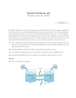
Numerous optimal properties among polynomials
deg(p) ≤ j, |p(t)| ≤ 1 for t ∈ [−1, 1] ⇒ |p(t)| ≤ |Tj (t)| for t 6∈ [−1, 1].
I.e., |Tj (t)| ≤ 1 for |t| ≤ 1 and |Tj (t)| grows fastest. (Sample plots next slide.)
where
Tj 1 + t =
1−t h
i
Tj t + 1 = 1 ∆j + ∆−j
t
t
t−1
2
for 1 6= t > 0,
√
t +1
for t > 0.
∆t := √
| t − 1|
Frequently show up in numerical analysis and computations: Chebyshev acceleration in
iterative methods, convergence of CG and Lanczos methods.
Chebyshev Polynomial (sample plots)
T0(t)
T1(t)
2
2
1.5
1
1
0
0.5
−1
T2(t)
8
6
4
2
0
−2
0
2
−2
−2
T3(t)
0
0
2
−2
−2
T4(t)
30
100
20
80
10
60
0
40
−10
20
−20
0
0
2
T5(t)
400
200
0
−200
−30
−2
0
2
−20
−2
0
2
−400
−2
0
2
Chebyshev Polynomial: typical use
Problem Given [α, β] and γ 6∈ [α, β], seek a polynomial p with deg(p) ≤ m such that
p(γ) = 1 and max |p(x)| is minimized.
x∈[α,β]
Define 1-1 mapping x ∈ [α, β] → t ≡ t(x) :=
t(γ) = −
Optimal p(x) =
1+
1−
α−γ
β−γ
α−γ
β−γ
2
β−α
for γ < α, and
x−
1+
1−
α+β
2
γ−β
γ−α
γ−β
γ−α
∈ [−1, 1],
for β < γ.
Tm (t(x))
:
Tm (t(γ))
p(γ) = 1,
√
1+ η
∆η =
√ ,
1− η
max |p(x)| =
x∈[α,β]
η=
α−γ
β−γ
h
i−1
1
,
= 2 ∆jη + ∆−j
η
|Tm (t(γ))|
for γ < α, and
η=
γ−β
γ−α
for β < γ.
Convergence Rate
Theorem on Convergence Rate (Golub & Ye, 2002)
Suppose λ1 is simple, i.e., λ1 < λ2 , and λ1 < ρ ℓ < λ2 . Let
ω1 < ω2 ≤ · · · ≤ ωn
be the eigenvalues of A − ρ ℓ B and v1 be an eigenvector corresponding to ω1 . Then
ρ ℓ − λ1 )ǫ2m + 2(ρ
ρ ℓ − λ1 )3/2 ǫm
ρ ℓ+1 − λ1 ≤ (ρ
kBk2
ω2
1/2
where
0 ≤ δℓ := ρ ℓ − λ1 + ω1
ǫm :=
min
v1H v1
v1H Bv1
ρ ℓ − λ1 |2 ),
= O(|ρ
max |f (ωj )|.
f ∈Pm−1 ,f (ω1 )=1 j>1
+ δℓ
Discussion
ǫm :=
min
f ∈Pm−1 ,f (ω1 )=1
maxj>1 |f (ωj )| usually unknown, except,
1 m = 2 for which the optimal fopt is
fopt (t) =
t − (ω2 + ωn )/2
∈ Pm−1 , fopt (ω1 ) = 1, max |fopt (ωj )| = |fopt (ω2 )| < 1.,
j>1
ω1 − (ω2 + ωn )/2
1−η
ω2 − ω1
ǫ2 =
, η=
.
1+η
ωn − ω1
2 ω2 = · · · = ωn for which fopt (t) = (t − ω2 )/(ω1 − ω2 ) and ǫm = 0 for all m ≥ 2.
In general ǫm can be bounded by using the Chebyshev polynomial
1+η
2t − (ωn + ω2 )
,
f (ω1 ) = 1,
Tm−1
ωn − ω2
1−η
−1
i
h
1+η
−(m−1) −1
.
= 2 ∆m−1
+ ∆η
≤ max |f (t)| = Tm−1
η
ω2 ≤tωn
1−η
f (t) = Tm−1
ǫm
Discussion
(cont’d)
ρ ℓ − λ1 )ǫ2m + 2(ρ
ρ ℓ − λ1 )3/2 ǫm
ρ ℓ+1 − λ1 ≤ (ρ
Ignoring high order terms,
kBk2
ω2
1/2
ρℓ − λ1 |2 ).
+ O(|ρ
ρ ℓ+1 − λ1
/ ǫ2m .
ρ ℓ − λ1
ρℓ − λ1 |2 ), quadratic convergence.
If ǫm = 0 (unlikely, however), then ρ ℓ+1 − λ1 = O(|ρ
Locally, ρ ℓ ≈ λ1 , eig(A − ρ ℓ B) ≈ eig(A − λ1 B) = {0 = γ1 < γ2 ≤ · · · ≤ γn }. So
ǫm ≈
min
h
i
−(m−1) −1
,
max |f (γj )| ≤ 2 ∆m−1
+ ∆η
η
f ∈Pm−1 ,f (γ1 )=1 j>1
∆η =
√
1+ η
√ ,
1− η
η=
γ2 − γ1
.
γn − γ1
Observation. ǫm depends on eig(A − ρ ℓ B), not on eig(A, B). This is the Key for
preconditioning later: transforming A − λB to preserve eig(A, B) but make
eig(A − ρ ℓ B) more preferable.
Key Lemma
Lemma (Golub & Ye, 2002)
Let (ω1 , v1 ) be the smallest eigenvalue of A − ρ ℓ B, i.e.. Then
− ω1
v1H v1
u H u1
≤ ρ ℓ − λ1 ≤ −ω1 H1
.
H
v1 Bv1
u1 Bu1
(4)
Asymptotically, if λ1 is a simple eigenvalue of A − λB, then as ρ ℓ → λ1 ,
ω1
v1H v1
v1H Bv1
= (λ1 − ρ ℓ ) + O(|λ1 − ρ ℓ |2 ).
Importance. Relate λ1 − ρ ℓ to ω1 . Special case: B = I , ω1 = λ1 − ρ ℓ .
(5)
Proof of Key Lemma
1) ρ ℓ ≥ λ1 always. If ρ ℓ = λ1 , then ω1 = 0. No proof needed.
2) Suppose ρℓ > λ1 . A − ρℓ B is indefinite and hence ω1 < 0. We have
(A − ρ ℓ B)v1 = ω1 v1 ,
(A − ω1 I − ρ ℓ B)v1 = 0,
A − ω1 I − ρ ℓ B 0.
ρℓ , v1 ) is the smallest eigenpair of (A − ω1 I ) − λB.
Therefore (ρ
3) Note also (λ1 , u1 ) is the smallest eigenpair of A − λB.
ρℓ =
v1H (A − ω1 I )v1
v1H Bv1
≥ min
x
λ1 =
x H Ax
x H Bx
u1H Au1
=
u1H Bu1
x H (A
≥ min
x
Together yielding −ω1
+
=
v1H Av1
v1H Bv1
−ω1 v1H v1
v1H Bv1
−ω1 v1H v1
v1H Bv1
= λ1 +
u1H (A − ρ ℓ B)u1
u1H u1
+
·
−ω1 v1H v1
,
v1H Bv1
u1H u1
u1H Bu1
+ ρℓ
u H u1
u H u1
− ρℓ B)x
+ ρ ℓ = ω1 · H1
+ ρℓ .
· H1
x Hx
u1 Bu1
u1 Bu1
v1H v1
u H u1
≤ ρ ℓ − λ1 ≤ −ω1 H1
.
H
v1 Bv1
u1 Bu1
Proof of Key Lemma
ρ ℓ ) = ω1 .
4) ω1 (t) = λmin (A − tB), for t near λ1 . Then ω1 (λ1 ) = 0 and ω1 (ρ
5) ω1 (λ1 ) = 0 is a simple eigenvalue of A − λ1 B. So ω1 (t) is differentiable in a
neighborhood of λ1 .
ρℓ ) = −
6) Expand ω1 (t) at ρ ℓ , sufficiently close to λ1 . Can prove ω1′ (ρ
ρ ℓ ) + σ1′ (ρ
ρℓ )(t − ρ ℓ ) + O(|t − ρ ℓ |2 )
ω1 (t) = ω1 (ρ
= ω1 −
v1H Bv1
v1H v1
(t − ρ ℓ ) + O(|t − ρ ℓ |2 ).
Setting t = λ1 ,
0 = ω1 (λ1 ) = ω1 −
from which
ω1
v1H v1
v1H Bv1
v1H Bv1
v1H v1
(λ1 − ρ ℓ ) + O(|λ1 − ρ ℓ |2 ),
= (λ1 − ρ ℓ ) + O(|λ1 − ρ ℓ |2 ).
v1H Bv1
v1H v1
. Hence
Convergence Rate
Theorem on Convergence Rate (Golub & Ye, 2002)
Suppose λ1 is simple, i.e., λ1 < λ2 , and λ1 < ρ ℓ < λ2 . Let
ω1 < ω2 ≤ · · · ≤ ωn
be the eigenvalues of A − ρ ℓ B and v1 be an eigenvector corresponding to ω1 . Then
ρ ℓ − λ1 )ǫ2m + 2(ρ
ρ ℓ − λ1 )3/2 ǫm
ρ ℓ+1 − λ1 ≤ (ρ
kBk2
ω2
1/2
where
0 ≤ δℓ := ρ ℓ − λ1 + ω1
ǫm :=
min
v1H v1
v1H Bv1
ρ ℓ − λ1 |2 ),
= O(|ρ
max |f (ωj )|.
f ∈Pm−1 ,f (ω1 )=1 j>1
+ δℓ
Proof
1) C = A − ρ ℓ B = V ΩV H (eigen-decomposition), V = [v1 , v2 , · · · , vn ] (orthogonal),
Ω = diag(ω1 , ω2 , · · · , ωn ).
2) Km ≡ Km (C , x ℓ ) = {f (C )xx ℓ , f ∈ Pm−1 }, and
ρ ℓ+1 = min
x∈Km
x H Ax
x H (A − ρ ℓ B)x
= ρ ℓ + min
H
x∈Km
x Bx
x H Bx
= ρ ℓ + min
f ∈Pm−1
x
xH
ℓ f (C )Cf (C )x ℓ
x
xH
ℓ f (C )Bf (C )x ℓ
.
(6)
3) Let fopt ∈ Pm−1 be the minimizing polynomial that defines ǫm . Then fopt (ω1 ) = 1
by the definition, and also ǫm = max |fopt (ωj )| < 1 because
j>1
f (t) =
t − (ω2 + ωn )/2
∈ Pm−1 , f (ω1 ) = 1, max |f (ωj )| = |f (ω2 )| < 1.
j>1
ω1 − (ω2 + ωn )/2
H
x
x
4) x H
ℓ (A − ρ ℓ B)x ℓ = 0 ⇒ that v1 x ℓ 6= 0 and hence fopt (C )x ℓ 6= 0 (why?). Thus
ρ ℓ+1 ≤ ρ ℓ +
= ρℓ +
2 (Ω)ΩV H x
x H Vfopt
x
xH
ℓ
ℓ fopt (C )Cfopt (C )x ℓ
= ρℓ + H ℓ
Hx
xH
x
x
ℓ
ℓ fopt (C )Bfopt (C )x ℓ
ℓ Vfopt (Ω)B1 fopt (Ω)V
2 (Ω)Ωy
y H fopt
y H fopt (Ω)B1 fopt (Ω)y
,
where B1 = V H BV , y = V Hx ℓ .
Proof
5) Write y = [ξ1 , ξ2 , . . . , ξn ]T = ξ1 e1 + ŷ , ŷ = [0, ξ2 , . . . , ξn ]T . We have
y H fopt (Ω)B1 fopt (Ω)y = (ξ1 e1 + ŷ )H fopt (Ω)B1 fopt (Ω)(ξ1 e1 + ŷ )
= ξ12 fopt (ω1 )2 e1H B1 e1 + 2ξ1 fopt (ω1 )e1H B1 fopt (Ω)ŷ
+ ŷ H fopt (Ω)B1 fopt (Ω)ŷ
= ξ12 β12 + 2ξ1 β2 + β32 ,
where
β12 = e1H B1 e1 = v1H Bv1 ,
β32 = ŷ H fopt (Ω)B1 fopt (Ω)ŷ ≤ max fopt (ωj )2 kB1 k2 kŷ k22 = ǫ2m kBk2 kŷ k22 ,
j>1
|β2 | = |e1H B1 fopt (Ω)ŷ | ≤ β1 β3 .
P
P
2
2
2
x
Note j ωj ξj2 = y H Ωy = x H
j>1 ωj ξj ≥ ω2 kŷ k2 .
ℓ (A − ρ ℓ B)x ℓ = 0 ⇒ |ω1 |ξ1 =
Hence
|ω1 | 1/2
1/2
β3 ≤ ǫm kBk2
|ξ1 |.
ω2
Proof
2 (Ω)Ωy = ξ 2 ω + ŷ H f
2
6) y H fopt
opt (Ω) Ωŷ , and
1 1
2
y H fopt
(Ω)Ωy =
X
j
2
ŷ H fopt
(Ω)Ωŷ =
X
j>1
2 (Ω)Ωy
y H fopt
y Hf
opt (Ω)B1 fopt (Ω)y
≤
=
2
ωj fopt
(ωj )ξℓ2 ≤
X
j
2
ωj fopt
(ωj )ξℓ2 ≤ ǫ2m
ωj ξj2 = y H Ωy = 0,
X
j>1
ωj ξj2 = ǫ2m |ω1 |ξ12 .
ξ12 ω1 + ŷ H fopt (Ω)2 Ωŷ
ξ12 β12 + 2|ξ1 |β1 β3 + β32
2|ξ1 |β1 β3 + β32
ω1
ŷ H fopt (Ω)2 Ωŷ
ω1
− 2 · 2 2
+ 2 2
β12
β1 ξ1 β1 + 2|ξ1 |β1 β3 + β32
ξ1 β1 + 2|ξ1 |β1 β3 + β32
ω1
ω1 2|ξ1 |β1 β3
ŷ H fopt (Ω)2 Ωŷ
− 2 ·
+
2
2
2
β1
β1
ξ1 β1
ξ12 β12
3/2
|ω1 |
|ω1 |
kBk2 1/2
ω1
+ 2 ǫ2m .
ǫm
≤ 2 +2
2
β1
β1
ω2
β1
≤
Proof
7) We have proved
2 (Ω)Ωy
y H fopt
y H fopt (Ω)B1 fopt (Ω)y
Note
ω1
β12
= ω1
v1H v1
v1H Bv1
≤
ω1
+2
β12
|ω1 |
β12
3/2
ǫm
kBk2
ω2
1/2
+
|ω1 | 2
ǫ .
β12 m
= (λ1 − ρ ℓ ) + O(|λ1 − ρ ℓ |2 ) by the lemma. Therefore
ρ ℓ+1 − λ1 ≤ ρ ℓ − λ1 +
2 (Ω)Ωy
y H fopt
y H fopt (Ω)B1 fopt (Ω)y
|ω1 | 3/2
|ω1 |
kBk2 1/2
ω1
+ 2 ǫ2m
ǫm
≤ ρ ℓ − λ1 + 2 +2
2
β1
β1
ω2
β1
{z
}
|
δℓ
ρ ℓ − λ1 )3/2 ǫm
≤ δℓ + 2(ρ
as expected.
kBk2
ω2
1/2
ρℓ − λ1 )ǫ2m ,
+ (ρ
What is Preconditioning?
Preconditioning. Transforming a problem that is “easier” (e.g., taking less time) to
solve iteratively.
Preconditioning natural for linear systems: transform Ax = b to KAx = Kb which is
“easier” than before. Extreme case: KA = I , i.e., K = A−1 , then x = Kb. But this is
impractical!
A comprise: make KA ≈ I as much as practical. Here KA ≈ I is understood either
kKA − I k is relatively small or KA − I is near a low rank matrix.
Preconditioning not so natural for eigenvalue problems: transform A − λB to
KA − λKB or LH AL − λLH BL which is “easier” than before.
No straightforward explanation as to what K makes KA − λKB “easier”
No straightforward explanation as to what L makes LH AL − λLH BL “easier”,
except L being the eigenvector matrix that is unknown. No easy way to
approximate the unknown eigenvector matrix either.
Will present two ways to understand eigen-problem preconditioning and construct
preconditioners.
Eigen-problem preconditioning, I
Ideal search direction p: starting at x ℓ , p points to the optimum, i.e., the optimum is
on the line {xx ℓ + tp : t ∈ C}. How can it be done with unknown optimum?
Expand x ℓ as a linear combination of uℓ
xℓ =
n
X
αj uj =: α1 u1 + v ,
v =
j=1
n
X
j=2
αj uj ⊥B u1 .
Then ideal p = αu1 + βvv , β 6= 0 such that α1 β − α 6= 0 (otherwise p = βxx ℓ ).
Ideal p has to be approximated to be practical. One such approximate p is
p = (A − σB)−1 r ℓ = (A − σB)−1 [A − ρ ℓ B]xx ℓ ,
where ρ ℓ 6= σ ≈ λ1 , also reasonably we assume σ 6= λj for all j > 1. Why so?
p=
n
X
µj αj uj ,
j=1
µj :=
λj − ρ ℓ
.
λj − σ
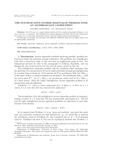
Now if λ1 ≤ ρℓ < λ2 and if the gap λ2 − λ1 is reasonably modest, then
µj ≈ 1
for j > 1
to give a p ≈ αv1 + v , resulting in fast convergence.
µj = (λj − ρℓ )/(λj − σ)
1
0.8
0.6
0.4
0.2
(t−1.01)/(t−0.99)
0
−0.2
−0.4
−0.6
−0.8
−1
1
2
3
4
5
6
7
8
9
10
Eigen-problem preconditioning, I
Preconditioner (A − σB)−1
P
Let x ℓ = nj=1 αj uj , and suppose α1 6= 0. If σ 6= ρ ℓ such that
either µ1 < µj for 2 ≤ j ≤ n or µ1 > µj for 2 ≤ j ≤ n,
where µj =
ρℓ
λj −ρ
,
λj −σ
then
h
i
−(m−1) −1
tan θB (u1 , Km ) ≤ 2 ∆m−1
tan θB (u1 , x ℓ ),
+ ∆η
η
h
i−2
−(m−1)
0 ≤ ρ ℓ+1 − λ1 ≤ 4 ∆m−1
tan θB (u1 , x ℓ ),
+ ∆η
η
where Km := Km ([A − σB]−1 [A − ρ ℓ B], x ℓ ), and

λn − σ λ2 − λ1


·
,

λn − λ1 λ2 − σ
η=

 λ2 − σ · λn − λ1 ,

λ2 − λ1 λn − σ
if µ1 < µj for 2 ≤ j ≤ n,
if µ1 > µj for 2 ≤ j ≤ n.
Discussion
η ≈ 1 (fast convergence) if σ ≈ λ1 . In fact η = 1 (implying ∆η = ∞) if σ = λ1 .
But shift σ needs to make µ1 either smallest or biggest among all µj . Three
interesting cases:
σ < λ1 ≤ ρ < λ2 , µ1 smallest
λ1 < σ < ρ < λ2 , µ1 biggest
λ1 < ρ < σ < λ2 , µ1 smallest.
(A − σB)−1 realized through linear system solving, but cost is high if solved
accurately, thus only approximately, such as
incomplete decompositions LDLH of A − σB with/without an iterative method
CG, MINRES
(more from Sherry Li’s lectures.)
Eigen-problem preconditioning, II
Use Golub and Ye’s Theorem (2002) as starting point:
ρ ℓ − λ1 )ǫ2m + 2(ρ
ρ ℓ − λ1 )3/2 ǫm
ρ ℓ+1 − λ1 ≤ (ρ
ǫm :=
min
kBk2
ω2
1/2
ρℓ − λ1 |2 ),
+ O(|ρ
max |f (ωj )|,
f ∈Pm−1 ,f (ω1 )=1 j>1
where ω1 < ω2 ≤ · · · ≤ ωn are the eigenvalues of A − ρ ℓ B.
Idea: Transform A − λB to L−1 (A − λB)L− H so that L−1 (A − ρ ℓ B)L− H has “better”
eigenvalue distribution, i.e., much smaller ǫm .
ρℓ − λ1 |2 ),
Ideal: ω2 = · · · = ωn , then ǫm = 0 for m ≥ 2 and thus ρ ℓ+1 − λ1 = O(|ρ
quadratic convergence.
A − ρ ℓ B = LDLH ⇒ L−1 (A − ρ ℓ B)L− H = D = diag(±1). Ideal but not practical:
1 A − ρ ℓ B = LDLH may not exist at all. It exists if all leading principle
submatrices are nonsingular.
2 A − ρ ℓ B = LDLH may not be numerically stable to compute, especially when
ρ ℓ ≈ λ1 .
3 L significantly denser than A and B combined. Ensuing computations are too
expensive.
Eigen-problem preconditioning, II
Compromise. A − ρ ℓ B ≈ LDLH with a good chance that
one smallest isolated eigenvalue ω1 , and the rest ωj (2 ≤ j ≤ n)
a few tight clusters.
Here A − ρ ℓ B ≈ LDLH includes not only the usual “approximately equal”, but also
when (A − ρ ℓ B) − LDLH approximately of a low rank.
L varies from one iterative step to another; Can be expensive; Possible to use constant
preconditioner, i.e., one L for all steps or change it every few steps.
Constant preconditioner: Use a shift σ ≈ λ1 , and perform an incomplete LDLH
decomposition of A − σB ≈ LDLH . Then
bℓ = L−1 (A − σB)L− H + (σ − ρ ℓ )L−1 BL− H ≈ D
C
would have a better spectral distribution so long as (σ − ρ ℓ )L−1 BL− H is small relative
bℓ .
to C
Insisted so far about applying ESD straightforwardly to the transformed problem
L−1 (A − λB)L− H . But there is alternative, perhaps better, way.
Eigen-problem preconditioning, II
b ℓ − λB
bℓ := L−1 (A − λB)L− H . Typical step of ESD for A
b ℓ − λB
bℓ :
A − λB to A
ℓ
ℓ
compute the smallest eigenvalue µ and corresponding eigenvector v of
b H (A
b ℓ − λB
bℓ )Z
b , where Z
b ∈ Cn×m is a basis matrix of Krylov subspace
Z
b
b
ρ
x
Km (Aℓ − ρ̂ ℓ Bℓ , x̂ ℓ ).
ij
h
j
H
bℓ x̂x ℓ = LH (Lℓ LH )−1 (A − ρ̂
b ℓ − ρ̂
x
ρℓ B) (L−
ρℓ B
Notice A
ℓ
ℓ
ℓ x̂ ℓ ) to see
H
H
H −1
b ℓ − ρ̂
bℓ , x̂x ℓ ) = Km ( Kℓ (A − ρ̂
ρℓ B
ρℓ B), x ℓ ), x ℓ = L−
x
.
L−
· Km (A
ℓ
ℓ x̂ ℓ , Kℓ = (Lℓ Lℓ )
Hb
ρℓ B), x ℓ ). Also
So Z = L−
Z is a basis matrix of Krylov subspace Km ( Kℓ (A − ρ̂
ℓ
b ) = Z H (A − λB)Z ,
b H (A
b ℓ − λB
bℓ )Z
b = (L− H Z
b )H (A − λB)(L− H Z
Z
ℓ
ℓ
ρℓ =
ρ̂
b xℓ
x
xH
x̂x H
ℓ Ax ℓ
ℓ Aℓx̂
= H
= ρℓ.
Hb
x ℓ Bxx ℓ
x̂x ℓ Bℓx̂x ℓ
The typical step can be reformulated equivalently to
compute the smallest eigenvalue µ and corresponding eigenvector v of
Z H (A − λB)Z , where Z ∈ Cn×m is a basis matrix of Krylov subspace
−1 .
Km ( Kℓ (A − ρℓ B), x ℓ ), where Kℓ = (Lℓ LH
ℓ)
Extended Preconditioned SD
Extended Preconditioned Steepest Descent method
Given an initial approximation x 0 to u1 , a relative tolerance rtol, and an integer
m ≥ 2, the algorithm attempts to compute an approximate eigenpair to (λ1 , u1 ) with
the prescribed rtol.
1: x 0 = x 0 /kxx 0 kB , ρ 0 = x H0 Axx 0 , r 0 = Axx 0 − ρ 0 Bxx 0 ;
2: for ℓ = 0, 1, . . . do
ρℓ | kBxx ℓ k2 ) ≤ rtol then
3:
if krr ℓ k2 /(kAxx ℓ k2 + |ρ
4:
BREAK;
5:
else
6:
construct a preconditioner Kℓ ;
7:
compute a basis matrix Z ∈ Cn×m of Krylov subspace
8:
9:
10:
11:
12:
13:
Km ( Kℓ (A − ρ ℓ B), x ℓ );
compute the smallest eigenvalue µ and corresponding eigenvector v of
Z H (A − λB)Z ;
y = Zv , x ℓ+1 = y /ky kB ;
ρ ℓ+1 = µ, r ℓ+1 = Axx ℓ+1 − ρ ℓ+1 Bxx ℓ+1 ;
end if
end for
ρ ℓ , x ℓ ) as an approximate eigenpair to (λ1 , u1 ).
return (ρ
It actually includes Eigen-problem preconditioning, I & II.
Convergence Rate
Theorem on Convergence Rate (Golub & Ye, 2002)
Suppose λ1 is simple, i.e., λ1 < λ2 , and λ1 < ρ ℓ < λ2 , and preconditioner Kℓ ≻ 0. Let
ω1 < ω2 ≤ · · · ≤ ωn
be the eigenvalues of Kℓ (A − ρ ℓ B) and v1 be an eigenvector corresponding to ω1 .
Then
ρℓ −
ρ ℓ+1 − λ1 ≤ (ρ
λ1 )ǫ2m
3/2
ρ ℓ − λ1 )
+ 2(ρ
ǫm
−H
kL−1
ℓ BLℓ k2
ω2
where
0 ≤ δℓ := ρ ℓ − λ1 + ω1
ǫm :=
min
v1H Kℓ−1 v1
v1H Bv1
ρℓ − λ1 |2 ),
= O(|ρ
max |f (ωj )|.
f ∈Pm−1 ,f (ω1 )=1 j>1
!1/2
+ δℓ
Discussion
ǫm :=
min
f ∈Pm−1 ,f (ω1 )=1
maxj>1 |f (ωj )| usually unknown, except,
1 m = 2 for which the optimal fopt is
f (t) =
t − (ω2 + ωn )/2
∈ Pm−1 , f (ω1 ) = 1, max |f (ωj )| = |f (ω2 )| < 1.,
j>1
ω1 − (ω2 + ωn )/2
1−η
ω2 − ω1
ǫ2 =
, η=
.
1+η
ωn − ω1
2 ω2 = · · · = ωn for which fopt (t) = (t − ω2 )/(ω1 − ω2 ) and ǫm = 0 for all m ≥ 2.
In general ǫm can be bounded by using the Chebyshev polynomial
1+η
2t − (ωn + ω2 )
,
f (ω1 ) = 1,
Tm−1
ωn − ω2
1−η
−1
i
h
1+η
−(m−1) −1
.
= 2 ∆m−1
+ ∆η
≤ max |f (t)| = Tm−1
η
ω2 ≤tωn
1−η
f (t) = Tm−1
ǫm
Discussion
(cont’d)
ρℓ −
ρ ℓ+1 − λ1 ≤ (ρ
λ1 )ǫ2m
3/2
ρ ℓ − λ1 )
+ 2(ρ
Ignoring high order terms,
ǫm
−H
kL−1
ℓ BLℓ k2
ω2
!1/2
ρℓ − λ1 |2 ).
+ O(|ρ
ρ ℓ+1 − λ1
/ ǫ2m .
ρ ℓ − λ1
ρℓ − λ1 |2 ), quadratically
If ǫm = 0 (unlikely, however), then ρ ℓ+1 − λ1 = O(|ρ
convergence.
Locally, ρ ℓ ≈ λ1 , eig(Kℓ (A − ρ ℓ B)) ≈ eig(Kℓ (A − λ1 B)) = {0 = γ1 < γ2 ≤ · · · ≤ γn },
and
ǫm ≈
min
i
h
−(m−1) −1
,
max |f (γj )| ≤ 2 ∆m−1
+ ∆η
η
f ∈Pm−1 ,f (γ1 )=1 j>1
∆η =
√
1+ η
√ ,
1− η
η=
γ2 − γ1
.
γn − γ1
Convergence Rate: Samokish Theorem
Theorem on Convergence Rate (Samokish, 1958)
m = 2, eig(Kℓ (A − λ1 B)) = {0 = γ1 < γ2 ≤ · · · ≤ γn }. Suppose λ1 is simple, i.e.,
λ1 < λ2 , and λ1 < ρ ℓ < λ2 ,
δ=
If τ
√
q
ρℓ − λ1 ],
kB 1/2 Kℓ B 1/2 k2 [ρ
γn + δ δ < 1, then
ρ ℓ+1 − λ1 ≤
where
η=
γ2 − γ1
,
γn − γ1
τ =
2
.
γ2 + γn
2
√
ǫ2 + τ γn δ
ρℓ − λ1 ],
[ρ
√
1 − τ ( γn + δ)δ
(7)
−1
1−η
ǫ2 = 2 ∆η + ∆−1
=
.
η
1+η
ρℓ − λ1 ), same as Golub & Ye (2002), but (7) is strict.
Asymptotically ρ ℓ+1 − λ1 / ǫ22 (ρ
Proof
1) topt = arg mint ρ(xx ℓ + tKℓ r ℓ ), y = x ℓ + topt Kℓr ℓ . Thus ρ ℓ+1 = ρ(y ).
2) Drop subscript ℓ to x , r , and K : r ℓ = r (xx ), ρ ℓ = ρ(xx ).
3) z = x − τ Kr (xx ). Then λ1 ≤ ρ(y ) ≤ ρ(z), thus ρ(y ) − λ1 ≤ ρ(z) − λ1 .
4) Suffices to show ρ(z) − λ1 ≤ RHS of (7).
5) A − λ1 B is symmetric positive semidefinite. k · kA−λ1 B is a semi-norm.
kw k2A−λ1 B = [ρ(w ) − λ1 ]kw k2B ,
k[I − τ K (A − λ1 B)]w kA−λ1 B ≤ ǫ2 kw kA−λ1 B .
6) Write z = [I − τ K (A − λ1 B)]xx + τ [ρ(xx ) − λ1 ]KBxx , and assume kxx kB = 1.
kzkA−λ1 B =
p
ρ(z) − λ1 kzkB ,
kzkA−λ1 B ≤ k[I − τ K (A − λ1 B)]xx kA−λ1 B + τ [ρ(xx ) − λ1 ]kKBxx kA−λ1 B
√
≤ ǫ2 kxx kA−λ1 B + τ [ρ(xx ) − λ1 ] γn kBxx kK
q
p
≤ ǫ2 ρ(xx ) − λ1 + τ [ρ(xx ) − λ1 ] γn kB 1/2 KB 1/2 k2
p
√
= (ǫ2 + τ γn δ) ρ(xx ) − λ1 .
Proof
(cont’d)
7) z = x − τ Kr (xx ), and kxx kB = 1.
kzkB ≥ kxx kB − τ kKr (xx )kB = 1 − τ kKr (xx )kB ,
kKr (xx )kB = kK (A − λ1 B)xx − [ρ(xx ) − λ1 ]KBxx kB
≤ kK (A − λ1 B)xx kB + [ρ(xx ) − λ1 ]kKBxx kB
q
≤ kK 1/2 BK 1/2 k2 γn kxx kA−λ1 B + [ρ(xx ) − λ1 ]kB 1/2 KB 1/2 k2 kxx kB
√
= γn δ + δ2 .
8) Finally use
ρ(z) − λ1 =
to complete the proof.
kzk2A−λ1 B
kzk2B
≤
kzk2A−λ1 B
[1 − τ kKr (xx )kB ]2
Deflation
So far computing (λ1 , u1 ) by single-vector steepest descent type methods.
To compute any following eigenpairs, must incorporate deflation techniques.
Or use a multi-vector/block method (not discussed yet). Deflation is also a necessary
tool to make a block method more efficient.
Assume acceptable approximations to (λi , ui ) for 1 ≤ j ≤ k known.
Diagonal D ∈ Rk×k holds known approximations of λi ,
U ∈ Rn×k holds known approximations of ui .
U = Ik .
Assume U H BU
Deflation: avoid computing (λi , ui ) for 1 ≤ j ≤ k, and seek approximation to
(λk+1 , uk+1 ). Will discuss two deflation techniques.
Through orthogonalizing against U
When the basis matrix Z is computed, make sure that Z is B-orthogonal to U . E.g.,
build a basis matrix Z for Km (K (A − ρB), x) such that U H ⊥B Z = 0. Suppose
x⊥B U = 0 already.
Arnoldi-like process
1: Z(:,1) = x/kxkB , ρ = x H Ax/kxk2B ;
2: for i = 2 to m do
3:
q = K (AZ(:,i −1) − ρBZ(:,i −1) );
U H (Bq));
4:
q = q − U (U
5:
for j = 1 to i − 1 do
H
6:
t = Z(:,i
Bq, q = q − Z(:,i −1) t;
−1)
7:
end for
8:
t = kqkB ;
9:
if t > 0 then
10:
Z(:,i ) = q/t;
11:
else
12:
BREAK;
13:
end if
14: end for
Note: Keep AZ for later use.
Through shifting λi away
Lemma
Let U1 = U(:,1:k) = [u1 , . . . , uk ]. (A + ζBU1 U1H B) − λB and A − λB share same
eigenvectors ui , but the eigenvalues of (A + ζBU1 U1H B) − λB are
λi + ζ for 1 ≤ i ≤ k and λi for k + 1 ≤ i ≤ n.
U U H B) − λB, where ζ should
Modify A − λB in form, but not explicitly, to (A + ζBU
be selected such that ζ + λ1 ≥ λk+2 .
But λk+2 is unknown. What we can do in practice to pick ζ a sufficiently large
number.
Block Steepest Descent Method
Block Steepest Descent Method
Block Extended Steepest Descent Method
Block Preconditioned Extended Steepest Descent Method
Why block versions
Single-vector SD and variations:
compute (λ1 , u1 ), and, with deflations, other (λi , ui ), one pair at a time. Most
computations are of matrix-vector type.
Slow convergence if (γ2 − γ1 )/(γn − γ1 ) tiny; usually happens when λ2 very
close to λ1 . (γi are eigenvalues of K (A − λ1 B).)
Often in practice, there are needs to compute the first few eigenpairs, not just
the first one.
Block versions:
Can simultaneously compute the first k eigenpairs (λj , uj );
Run more efficiently on modern computer architecture: more computations in
matrix-matrix multiplication type;
Better rates of convergence; can save overall cost by using a block size that is
slightly bigger than the number of asked eigenpairs.
In summary, the benefits of using a block variation are similar to those of using the
simultaneous subspace iteration vs. the power method.
Block SD
Start with X0 ∈ Cn×nb , rank(X0 ) = nb ≥ k, instead of just one vector x 0 ∈ Cn .
May assume jth column of X0 approximates uj ; otherwise R(X0 ) approximates
span{u1 , . . . , unb }. In the latter, preprocessing X0 :
1 compute eigen-decomposition (X0H AX0 ) W = (X0H BX0 ) W Ω, where
Ω = diag(ρ0;1 , ρ0;2 , . . . , ρ0;nb );
2 Reset X0 := X0 W .
Can always assume jth column of X0 approximates uj .
Typical ℓth iterative step: already have
Xℓ = [xℓ;1 , xℓ;2 , . . . , xℓ;nb ] ∈ Cn×nb ,
Ωℓ = diag(ρℓ;1 , ρℓ;2 , . . . , ρℓ;nb ),
jth column xℓ;j approximates uj ,
ρℓ,j = ρ(xℓ;j ) ≈ λj .
To compute new approximations as follows.
1 Compute a basis matrix Z of R([Xℓ , Rℓ ]) by, e.g., MGS in the B-inner product,
keeping in mind that Xℓ is B-orthonormal already;
2 Find the first nb eigenpairs of Z H AZ − λZ H BZ to get
(Z H AZ )W = (Z H BZ )W Ωℓ+1 , Ωℓ+1 = diag(ρℓ+1;1 , ρℓ+1;2 , . . . , ρℓ+1;nb );
3 Set Xℓ+1 = ZW .
Block Extended SD
Block SD (previous slide) is is the stronger version of Simultaneous Rayleigh
Quotient Minimization Method of Longsine and McCormick (1980).
Note that r (xℓ;j ) = (A − ρℓ;j B)xℓ;j and thus
R([Xℓ , Rℓ ]) =
nb
X
j=1
R([xℓ;j , (A − ρℓ;j B)xℓ;j ]) =
nb
X
j=1
K2 (A − ρℓ;j B, xℓ;j ).
Naturally, as before, to expand search space, R([Xℓ , Rℓ ]) through extending each
K2 (Axℓ;j − ρℓ;j B, xℓ;j ) to a high order one. The new extended search subspace now is
nb
X
j=1
Km (A − ρℓ;j B, xℓ;j ) = span{Xℓ , Rℓ (Xℓ ), . . . , Rℓm−1 (Xℓ )} =: Km (Rℓ , Xℓ ),
where the linear operator Rℓ : X ∈ Cn×nb → Rℓ (X ) = AX − BX Ωℓ ∈ Cn×nb .
Rℓi ( · ) = Rℓi −1 (Rℓ ( · )), e.g., Rℓ2 (X ) = Rℓ (Rℓ (X )).
Block Extended SD: make Z basis matrix of Km (Rℓ , Xℓ ).
Incorporate Preconditioners
In light of extensive discussions on preconditioning, natural to modify the search
subspace to
nb
X
Km (Kℓ;j (A − ρℓ;j B), xℓ;j ),
j=1
where Kℓ;j is the preconditioner intended to move (ρℓ;j , xℓ;j ) towards (λj , uj ) faster for
each j.
Two ways to construct Kℓ;j :
Kℓ;j ≈ (A − ρ̃ℓ;j B)−1 for some ρ̃ℓ;j 6= ρℓ;j , ideally closer to λj than to any other
eigenvalue of A − λB.
Since the eigenvalues of A − λB are unknown, practically make ρ̃ℓ;j closer but
not equal to ρℓ;j than to any other ρℓ;k .
Perform incomplete LDLH factorization: A − ρℓ;j B ≈ Lℓ;j Dℓ;j LH
ℓ;j , where “≈”
includes not only the usual “aproximately equal”, but also the case when
(A − ρℓ;j B) − Lℓ;j Dℓ;j LH
ℓ;j is approximately a low rank matrix, and
Dℓ;j = diag(±1).
Finally, Ki :j = Lℓ;j LH
ℓ;j .
Block Preconditioned Extended SD
Block Preconditioned Extended Steepest Descent method
Given an initial approximation X0 ∈ Cn×nb with rank(X0 ) = nb , and an integer m ≥ 2,
the algorithm attempts to compute approximate eigenpair to (λj , uj ) for 1 ≤ j ≤ nb .
1: compute the eigen-decomposition: (X0H AX0 )W = (X0H BX0 )W Ω0 ,
where W H (X0H BX0 )W = I , Ω0 = diag(ρ0;1 , ρ0;2 , . . . , ρ0;nb );
2: X0 = X0 W ;
3: for ℓ = 0, 1, . . . do
4:
test convergence and lock up the converged (detail to come later);
5:
construct preconditioners Kℓ;j for 1 ≤ j ≤ nb ;
nb
X
Km (Kℓ;j (A − ρℓ;j B), xℓ;j );
6:
compute a basis matrix Z ∈ Cn×mnb of
j=1
7:
compute the nb smallest eigenvalues and corresponding eigenvectors of
Z H (A − λB)Z to get (Z H AZ )W = (Z H BZ )W Ωℓ , where W H (Z H BZ )W = I ,
Ωℓ+1 = diag(ρℓ+1;1 , ρℓ+1;2 , . . . , ρℓ+1;nb );
8:
Xℓ+1 = ZW ;
9: end for
10: return approximate eigenpairs to (λj , uj ) for 1 ≤ j ≤ nb .
Implementation Issue, I
Different preconditioner Kℓ;j for each different approximate eigenpair (ρℓ;j , xℓ;j ) good
for convergence rates, but may not reduce overall time:
expensive to construct all preconditioners
cannot compute Z mostly by matrix-matrix multiplications (more later)
Use Kℓ;j ≡ Kℓ , one preconditioner for all speeding up the convergence of (ρℓ;1 , xℓ;1 ).
At the same time other (ρℓ;j , xℓ;j ) are making progress, too, but at a slower speed.
Usually (ρℓ;1 , xℓ;1 ) converges first and quickly.
Once (ρℓ;1 , xℓ;1 ) (or the first few in the case of a tight cluster) is determined to be
sufficiently accurate, the converged eigenpair is locked up and deflated.
A new preconditioner is computed to aim at the next non-converged eigenpair, and
the process continues.
Implementation Issue, II
Need to compute basis matrix Z ∈ Cn×mnb of
nb
X
j=1
Km (Kℓ;j (A − ρℓ;j B), xℓ;j ).
Z can be gotten by packing the basis matrices of all Km (Kℓ;j (A − ρℓ;j B), xℓ;j ) for
1 ≤ j ≤ nb together. Two drawbacks:
Such a Z could be ill-conditioned, i.e., columns of Z may not be sufficiently
numerically linearly independent; Possible cure: re-orthogonalize packed Z – too
costly.
Building basis for each Km (Kℓ;j (A − ρℓ;j B), xℓ;j ) uses mostly BLAS-2
operations. Have to be this way if Kℓ;j are different.
Different situation if Kℓ;j ≡ K (drop iteration step index ℓ). Then
nb
X
j=1
Km (K (A − ρℓ;j B), xℓ;j ) = Km (K R, X )
≡ span{X , K R(Xℓ ), . . . , [K R]m−1 (X )},
where R(X ) = AX − BX Ω, [K R]i ( · ) = [K R]i (K R( · )), e.g.,
[K R]2 (X ) = K Rℓ (K R(X )).
Implementation Issue, II
(cont’d)
Z = [Z1 , Z2 , . . . , Zm ] can be computed by the following block Arnoldi-like process in
the B-inner product.
Arnoldi-like process for Z
1: Z1 = X (recall X H BX = Inb already);
2: for i = 2 to m do
3:
Y = K (AZi −1 − BΩZi −1 );
4:
for j = 1 to i − 1 do
5:
T = ZjH BY ; Y = Y − Zj T ;
6:
end for
7:
Zi T = Y (MGS in the B-inner product);
8: end for
Note: At Line 7, Y may not be numerically of full column rank – not a problem.
Anytime if a column is deemed linearly dependent on previous columns, that column
should be deleted, along with corresponding ρj from Ω.
At completion of MGS, Zj+1 will have fewer columns than Y and the size of Ω is
shrunk accordingly.
Implementation Issue, III
krℓ;j k2
≤ rtol.
kAxℓ;j k2 + |ρℓ;j | kBxℓ;j k2
Usually λj are converged to in order, i.e., the smallest eigenvalues emerge first.
(ρℓ;j , xℓ;j ) is considered acceptable if
Lock all acceptable approximate eigenpairs in kcvgd × kcvgd diagonal matrix D for
eigenvalues and n × kcvgd tall matrix U for eigenvectors.
Every time a converged eigenpair is detected, delete the converged ρℓ;j and xℓ;j from
Ωℓ and Xℓ , respectively, and expand D and U to lock up the pair, accordingly.
At the same time, either reduce nb by 1 or append a (random) B-orthogonal column
to X to maintain nb unchanged.
Deflate to avoid recomputing converged eigenpairs:
1 At Line 7 in the Arnoldi-like process, each column of Zj+1 is B-orthogonalized
against U .
U U H B) − λB, where ζ
2 Modify A − λB in form, but not explicitly, to (A + ζBU
should be selected such that ζ + λ1 ≥ λkcvgd +nb +1 . Here we pre-assume the
kcvgd converged eigenpairs are indeed those for (λj , uj ) for 1 ≤ j ≤ kcvgd . This is
usually so, but with no guarantee, of course.
Conjugate Gradient Methods
Digression: CG for Linear System Ax = b
Conjugate Gradient Method
Preconditioned Conjugate Gradient Method
Locally Optimal Conjugate Gradient Method
Locally Optimal Extended Conjugate Gradient Method
Locally Optimal Block Preconditioned Extended Conjugate
Gradient Method
CG for Linear System Ax = b
A is n × n, symmetric, and positive definite. Let
φ(x) =
1 T
x Ax − x T b,
2
quadratic in x, convex, a unique local and global minimum at x = A−1 b,
∇φ(x) = r (x) ≡ Ax − b.
CG Algorithm (Hestenes and Stiefel, 1950s):
1 Given x0 , compute r0 = Ax0 − b, and set p0 = −r0 ;
2 For i = 0, 1, . . ., do
αi = arg min φ(xi + αpi ),
α
ri +1 = ri + αi Api ,
xi +1 = xi + αi pi ,
pi +1 = −ri +1 + βi pi .
βi chosen so that piT+1 Api = 0; equivalent expressions:
βi =
piT Ari +1
piT Api
=
riT+1 ri +1
riT ri
=
riT+1 (ri +1 − ri )
riT ri
.
Nonlinear CG
Verbatim translations of Hestenes’ and Stiefel’s CG to solve
min φ(x),
x
φ(x) not necessarily quadratic,
replacing all r (xi ) by ∇φ(xi ).
Nonlinear CG Algorithm (Fletcher and Reeves, 1964):
1 Given x0 , compute ∇φ0 = ∇φ(x0 ), and set p0 = −∇φ0 ;
2 For i = 0, 1, . . ., do
αi = arg min φ(xi + αpi ),
xi +1 = xi + αi pi ,
evaluate ∇φi +1 = ∇φ(xi +1 ),
pi +1 = −∇φi +1 + βi pi .
α
Several choices for βi :
βi =
∇φT
i +1 ∇φi +1
∇φT
i ∇φi
,
βi =
∇φT
i +1 (∇φi +1 − ∇φi )
∇φT
i ∇φi
.
Locally Optimal CG
Linear CG: choices of βi make
search directions pi conjugate, i.e., piT Apj = 0 for i 6= j.
CG method terminates in at most n steps.
Nonlinear CG: many nice properties no longer hold for any choice of βi .
Observe
xi +2 = xi +1 + αi +1 (−∇φi +1 + βi pi )
∈ span{xi +1 , ∇φi +1 , pi } = span{xi +1 , ∇φi +1 , xi }.
Since many nice properties in linear CG are lost anyway in the nonlinear case, why not
pick βi , implicitly, such that (Takahashi, 1965)
xi +2 =
arg min
φ(y ).
y∈span{xi +1 ,∇φi +1 ,xi }
This gives locally optimal CG. But search over y ∈ span{xi +1 , ∇φi +1 , xi } harder than
before.
CG for Ax = λBx
Minimize ρ(x) to compute (λ1 , u1 ):
ρ(x) =
x H Ax
,
x H Bx
∇ρ(x) =
2
r (x),
x H Bx
r (x) := Ax − ρ(x) Bx.
Line-search ρ(y ) = inf ρ(x + tp)
t∈C
1: compute the smaller eigenvalue µ of X H AX − λX H BX , where X = [x, p], and
eigenvector v = [ν1 , ν2 ]T ; (
ν /ν ,
2: arg inf ρ(x + tp) =: topt = 2 1
∞,
t∈C
(
x + topt p
if topt is finite,
3: y =
p
otherwise.
if ν1 6= 0,
if ν1 = 0;
CG for Ax = λBx: in nonlinear CG simply replace ∇φ(x) by r (x) := Ax − ρ(x) Bx.
CG for Ax = λBx
CG for Ax = λBx
Given an initial approximation x 0 to u1 , and a relative tolerance rtol, the algorithm
attempts to compute an approximate eigenpair to (λ1 , u1 ) with the prescribed rtol.
1: x 0 = x 0 /kxx 0 kB , ρ 0 = x H0 Axx 0 , r 0 = Axx 0 − ρ 0 Bxx 0 , p 0 = −rr 0 ;
2: for ℓ = 0, 1, . . . do
ρℓ | kBxx ℓ k2 ) ≤ rtol then
3:
if krr ℓ k2 /(kAxx ℓ k2 + |ρ
4:
BREAK;
5:
else
p ℓ ), and then
6:
compute αℓ = topt := inf ρ(xx ℓ + tp
t∈C
(
x ℓ + αℓp ℓ
if αℓ is finite,
y=
pℓ
otherwise.
7:
x ℓ+1 = y /ky kB ;
x
x
x
r
8:
set ρ ℓ+1 = x H
ℓ+1 Ax ℓ+1 , r ℓ+1 = Ax ℓ+1 − ρ ℓ+1 Bx ℓ+1 , p ℓ+1 = −r ℓ+1 + βℓp ℓ ,
where βℓ =
rH
ℓ+1 r ℓ+1
rH
r
ℓ ℓ
or
rH
ℓ+1 (rr ℓ+1 −rr ℓ )
rH
r
ℓ ℓ
9:
end if
10: end for
11: return (ρρ ℓ , x ℓ ) as an approximate eigenpair to (λ1 , u1 ).
A Convergence Theorem
Convergence Theorem (Yang, 1993)
With βℓ =
rH
ℓ+1 r ℓ+1
rH
r
ℓ ℓ
, ρ ℓ converges to some eigenvalue λ̂ of A − λB and there is a
convergent subsequence {xx ℓi } of {xx ℓ } such that
k(A − λ̂B)xx ℓi k2 → 0
as
i → ∞,
i.e., x ℓi converges in direction to a corresponding eigenvector.
If λ̂ = λ1 , then k(A − λ̂B)xx ℓ k2 → 0 as ℓ → ∞, i.e., x ℓ converges in direction to a
corresponding eigenvector. (seem new)
First part due to (Yang, 1993); second part seems new.
Only for βℓ =
rH
ℓ+1 r ℓ+1
rH
r
ℓ ℓ
, however.
Proof much more complicated than for SD.
Rate of convergence: mostly heuristic, none rigorous proven.
Preconditioned CG for Ax = λBx
As in SD, Preconditioned CG = vanilla CG on L− H AL−1 − λL− H BL−1 .
e − λB
e := L− H AL−1 − λL− H BL−1 . Adopt notation convention for A
e − λB:
e
Let A
same symbols but with tildes. E.g., e
x = Lx,
ρe(e
x) =
e
x H L− H AL−1 e
x
≡ ρ(x),
e
x H L− H BL−1 e
x
Key CG step:
e
x ≡ L− H r (x).
x − ρe(e
x )L− H BL−1 e
r (e
x ) = L− H AL−1 e
eℓ ),
α
eℓ = arg min ρe(e
xℓ + α
ep
α
e
e
x ℓ+1 )L− H BL−1xeℓ+1 ,
r ℓ+1 = L− H AL−1xeℓ+1 − ρe(e
Perform substitutions xeℓ = Lxx ℓ and e
r ℓ = L− Hr ℓ :
eℓ ),
α
eℓ = arg min ρ(xx ℓ + α
e L−1p
| {z }
α
e
pℓ
=:p
r ℓ+1 = Axx ℓ+1 − ρ(xx ℓ+1 )Bxx ℓ+1 ,
eℓ ,
xeℓ+1 = xeℓ + α
eℓ p
eℓ .
eℓ+1 = −e
p
r ℓ+1 + βeℓp
eℓ ,
x ℓ+1 = x ℓ + α
eℓ L−1p
eℓ+1 = − (LH L)−1 r ℓ+1 + βeℓ L−1p
eℓ .
L−1p
| {z }
| {z }
| {z }
p ℓ+1
=:p
=:K
pℓ
=:p
Preconditioned CG for Ax = λBx
Preconditioned CG for Ax = λBx
Given an initial approximation x 0 to u1 , a (positive definite) preconditioner K , and a
relative tolerance rtol, the algorithm attempts to compute an approximate pair to
(λ1 , u1 ) with the prescribed rtol.
1: x 0 = x 0 /kxx 0 kB , ρ 0 = x H0 Axx 0 , r 0 = Axx 0 − ρ 0 Bxx 0 , p 0 = −Krr 0 ;
2: for ℓ = 0, 1, . . . do
ρℓ | kBxx ℓ k2 ) ≤ rtol then
3:
if krr ℓ k2 /(kAxx ℓ k2 + |ρ
4:
BREAK;
5:
else
p ℓ ), and then
6:
compute αℓ = topt := inf ρ(xx ℓ + tp
t∈C
(
x ℓ + αℓp ℓ
if αℓ is finite,
y=
pℓ
otherwise.
7:
x ℓ+1 = y /ky kB ;
x
x
x
8:
set ρ ℓ+1 = x H
ℓ+1 Ax ℓ+1 , r ℓ+1 = Ax ℓ+1 − ρ ℓ+1 Bx ℓ+1 ,
p ℓ+1 = −Krr ℓ+1 + βℓp ℓ , where βℓ =
rH
ℓ+1 Krr ℓ+1
rH
Krr ℓ
ℓ
or
9:
end if
10: end for
11: return (ρρ ℓ , x ℓ ) as an approximate eigenpair to (λ1 , u1 ).
rH
ℓ+1 K (rr ℓ+1 −rr ℓ )
.
rH
Krr ℓ
ℓ
Convergence
Earlier discussions on selecting a good preconditioner for PSD should apply:
A − σB = LDLH , D = diag(±1), K = (LH L)−1 .
Various heuristics on the convergence rates of the preconditioned CG, but none is
rigorously proved. Even less can be said about the theoretical analysis of block (or
subspace) versions of the preconditioned CG method (to come soon).
But since preconditioned CG is CG for L− H AL−1 − λL− H BL−1 , previous convergence
theorem for CG remains valid.
Locally Optimal CG for Ax = λBx
In writing down CG for Ax = λBx, we did
gradient-to-residual replacement: replacing the gradient by the eigen-residual
r (x) = Ax − ρ(x)Bx which differs by a scalar factor 2/x H Bx from the gradient
∇ρ(x) = x H2Bx [Ax − ρ(x) Bx];
also normalizing x ℓ . No theory around as to why we should normalize x ℓ , beside
that they are some eigenvector approximations.
We made a couple of “arbitrary choices”. Their effects on the rate of convergence are
not clear.
Locally optimal CG eliminates the “arbitrariness” altogether: compute x ℓ+1 from the
subspace span{xx ℓ−1 , x ℓ , r ℓ } by
min
x∈ span{xx ℓ−1 ,xx ℓ ,rr ℓ }
ρ(x),
which is solvable through the Rayleigh-Ritz procedure.
Locally Optimal CG
Locally Optimal CG for Ax = λBx
Given an initial approximation x 0 to u1 , and a relative tolerance rtol, the algorithm
attempts to compute an approximate eigenpair to (λ1 , u1 ) with the prescribed rtol.
1: x 0 = x 0 /kxx 0 kB , ρ 0 = x H0 Axx 0 , r 0 = Axx 0 − ρ 0 Bxx 0 , x −1 = 0;
2: for ℓ = 0, 1, . . . do
ρℓ | kBxx ℓ k2 ) ≤ rtol then
3:
if krr ℓ k2 /(kAxx ℓ k2 + |ρ
4:
BREAK;
5:
else
6:
compute a basis matrix Z ∈ Cn×k (k = 2 or 3) of the subspace
span{xx ℓ , x ℓ−1 , r ℓ };
7:
compute the smallest eigenvalue µ and corresponding eigenvector v of
Z H (A − λB)Z ;
8:
y = Zv , x ℓ+1 = y /ky kB ;
9:
ρ ℓ+1 = µ, r ℓ+1 = Axx ℓ+1 − ρ ℓ+1 Bxx ℓ+1 ;
10:
end if
11: end for
12: return (ρρ ℓ , x ℓ ) as an approximate eigenpair to (λ1 , u1 ).
Implementation
x ℓ moves closer and closer to u1 ; x ℓ , x ℓ−1 increasingly move towards being linearly
dependent.
Line 6: Z contaminated more and more by rounding errors. How to mitigate that?
To replace x ℓ−1 by some y ℓ := ξℓ,1x ℓ − ξℓ,2x ℓ−1 such that
span{xx ℓ , x ℓ−1 , r ℓ } = span{xx ℓ , y ℓ , r ℓ }.
Then same (µ, v ) at Line 7. But need to generate y ℓ+1 , given x ℓ , y ℓ , r ℓ .
Z = [z1 , z2 , z3 ] is B-orthonormal (by MGS), and z1 = x ℓ . Then
y = Zv = ν1 z1 + ν2 z2 + ν3 z3 = ν1 x ℓ + ν2 z2 + ν3 z3 .
Set y ℓ+1 := y − ν1x ℓ = ky kB x ℓ+1 − ν1x ℓ =: ξℓ+1,1x ℓ+1 − ξℓ+1,2x ℓ .
Modify Lines 1, 6, and 8 as follows while keeping others the same.
1: x 0 = x 0 /kxx 0 kB , ρ 0 = x H0 Axx 0 , r 0 = Axx 0 − ρ 0 Bxx 0 , y 0 = 0;
6:
compute a basis matrix Z ∈ Cn×k (k = 2 or 3) of the subspace
8:
span{xx ℓ , y ℓ , r ℓ };
y = Zv , x ℓ+1 = y /ky kB , y ℓ+1 = Z v̂ , where v̂ is v with its 1st entry zeroed;
Convergence
Convergence Theorem for LOCG)
ρ ℓ converges to some eigenvalue λ̂ of A − λB and k(A − λ̂B)xx ℓ k2 → 0 as ℓ → ∞, i.e.,
x ℓ converges in direction to a corresponding eigenvector.
Same convergence theorem for SD;
For CG, PCG, only k(A − λ̂B)xx ℓi k2 → 0;
Inclusion of the residual r ℓ makes the difference.
Improve LOCG
Three ideas for improving SD naturally apply here:
1 Incorporate a preconditioner K : simply modify r ℓ to Krr ℓ ;
2 Extend search space from currently
span{xx ℓ−1 } + K2 (A − ρℓ B, x ℓ )
to
span{xx ℓ−1 } + Km (A − ρℓ B, x ℓ );
3 Use block X0 ∈ Cn×nb .
The ideas can be applied in any combination (23 = 8 of them): E.g.,
Locally Optimal Preconditioned CG (LOPCG): m = 2, nb = 1, K 6= I ;
Locally Optimal Block Preconditioned CG (LOBPCG): m = 2, nb > 1, K 6= I ;
Locally Optimal Extended CG (LOECG): m > 2, nb = 1, K = I ;
Locally Optimal Preconditioned Extended CG (LOPECG): m > 2, nb = 1,
K 6= I ;
Locally Block Optimal Preconditioned Extended CG (LOBPECG): m > 2,
nb > 1, K 6= I .
Locally Optimal CG
Extended Locally Block Optimal Preconditioned CG
Given an initial approximation X0 ∈ Cn×nb with rank(X0 ) = nb , and an integer m ≥ 2,
the algorithm attempts to compute approximate eigenpairs to (λj , uj ) for 1 ≤ j ≤ nb .
1: compute the eigen-decomposition: (X0H AX0 )W = (X0H BX0 )W Ω0 , where
W H (X0H BX0 )W = I , Ω0 = diag(ρ0;1 , ρ0;2 , . . . , ρ0;nb );
2: X0 = X0 W , and X−1 = 0;
3: for ℓ = 0, 1, . . . do
4:
test convergence and lock up the converged (detail as in EBPSD);
5:
construct preconditioners Kℓ;j for 1 ≤ j ≤ nb ;
6:
compute a basis matrix Z ∈ Cn×(m+1)nb of the subspace
nb
X
j=1
7:
Km (Kℓ;j (A − ρℓ;j B), xℓ;j ) + R(Xℓ−1 );
compute the nb smallest eigenvalues and corresponding eigenvectors of
Z H (A − λB)Z to get (Z H AZ )W = (Z H BZ )W Ωℓ , where W H (Z H BZ )W = I ,
Ωℓ+1 = diag(ρℓ+1;1 , ρℓ+1;2 , . . . , ρℓ+1;nb );
8:
Xℓ+1 = ZW ;
9: end for
10: return approximate eigenpairs to (λj , uj ) for 1 ≤ j ≤ nb .
Implementation
Three important implementation issues earlier for XBPSD essentially apply here, but
more need to be said about Z at Line 6 here.
Xℓ−1 can be replaced by something else, using the idea earlier for LOCG. Specifically,
Lines 2, 6, and 8 should be modified to
2: X0 = X0 W , and Y0 = 0;
6:
compute a basis matrix Z ∈ Cn×(m+1)nb of the subspace
nb
X
j=1
8:
Km (Kℓ;j (A − ρℓ;j B), xℓ;j ) + R(Yℓ ) such that R(Z(:,1:nb ) ) = R(Xℓ );
c , where W
c is W with its nb rows zeroed;
Xℓ+1 = ZW , Yℓ+1 = Z W
For Kℓ;j ≡ Kℓ , Z is basis matrix of (dropping the subscript ℓ)
Km (K R, X ) + R(Y ) = span{X , K R(X ), . . . , [K R]m−1 (X )} + R(Y ).
1 compute a basis matrix [Z1 , Z2 , . . . , Zm ] for Km (K R, X ) by the Block
Arnoldi-like process in the B-inner product. In particular, Z1 = X .
2 B-orthogonalize Y against [Z1 , Z2 , . . . , Zm ] to get Zm+1 satisfying
H BZ
Zm+1
m+1 = I .
3 Z = [Z1 , Z2 , . . . , Zm+1 ].
References
Precise rates of convergence for various CG methods are scarce and not well
understood, especially so for methods of block version. The existing research on the
convergence of various SD and CG-type methods, although fragmental and
incomplete, should be helpful and provide heuristic insights. Some of the references are
L. Bergamaschi, G. Gambolati, and G. Pini. Asymptotic convergence of conjugate gradient methods for the
partial symmetric eigenproblem. Numer. Linear Algebra Appl., 4(2):69–84, 1997.
J. H. Bramble, J. E. Pasciak, and A. V. Knyazev. A subspace preconditioning algorithm for
eigenvector/eigenvalue computation. Adv. in Comput. Math., 6:159–189, 1996.
Andrew V. Knyazev and Klaus Neymeyr. A geometric theory for preconditioned inverse iteration III: A short
and sharp convergence estimate for generalized eigenvalue problems. Linear Algebra Appl., 358(1-3):95–114,
2003.
D. E. Longsine and S. F. McCormick. Simultaneous Rayleigh-quotient minimization methods for
Ax = λBx. Linear Algebra Appl., 34:195–234, 1980.
S. Oliveira. On the convergence rate of a preconditioned subspace eigensolver. Computing, 63:219–231,
1999.
E. E. Ovtchinnikov. Jacobi correction equation, line search, and conjugate gradients in hermitian eigenvalue
computation I: Computing an extreme eigenvalue. SIAM J. Numer. Anal., 46(5):2567–2592, 2008.
E. E. Ovtchinnikov. Jacobi correction equation, line search, and conjugate gradients in hermitian eigenvalue
computation II: Computing several extreme eigenvalues. SIAM J. Numer. Anal., 46(5):2593–2619, 2008.
H. Yang. Conjugate gradient methods for the Rayleigh quotient minimization of generalized eigenvalue
problems. Computing, 51:79–94, 1993.
Extending Min-Max Principles: Indefinite B
Early Extensions
Positive Semi-definite Pencil
Early Extensions
Min-max principles, Cauchy interlace inequalities are Foundations for optimization
approaches to solve few extreme eigenpairs of A − λB with B ≻ 0.
How far can these theoretical results be extended?
Early extensions (before 1982) of Courant-Fischer min-max princples:
Ax = λx with A 0 in an indefinite inner product
R. S. Phillips. A minimax characterization for the eigenvalues of a positive symmetric operator in a
space with an indefinite metric. J. Fac. Sci. Univ. Tokyo Sect. I, 17:51–59, 1970.
B. Textorius. Minimaxprinzipe zur Bestimmung der Eigenwerte J-nichtnegativer Operatoren. Math.
Scand., 35:105–114, 1974.
It turns out to be a special case of A − λB with indefinite and nonsingular B.
Hyperbolic Q(λ) = Aλ2 + Bλ + C :
R. Duffin. A minimax theory for overdamped networks. Indiana Univ. Math. J., 4:221–233, 1955.
More general nonlinear eigenvalue problems:
H. Voss and B. Werner. A minimax principle for nonlinear eigenvalue problems with applications to
nonoverdamped systems. Math. Meth. Appl. Sci., 4:415–424, 1982.
and references therein.
Will focus on A − λB with indefinite B and hyperbolic Q(λ) ...
Hermitian Ax = λBx with Indefinite B
Difficulties:
B is indefinite — Ax = λBx not equivalent to standard
Hermitian eigenvalue problem;
Ax = λBx may have complex eigenvalues — no min-max for
complex eigenvalues;
The case we consider will turn out to have only real
eigenvalues.
A − λB may be a singular pencil: det(A − λB) ≡ 0 for λ ∈ C.
Need a definition for eigenvalues.
History
1 Extending Courant-Fischer for regular Hermitian pencil:
Nonsingular B: Lancaster & Ye (1989), Ye’s thesis (1989), Najman & Ye
(1991), Binding & Ye (1995)
Singular B: Najman & Ye (1993), Binding & Najman & Ye (1999)
Only certain real semi-simple eigenvalues admit a Courant-Fischer type
characterization.
2 Extending trace min for positive semi-definite Hermitian pencil (i.e.,
A − λ0 B 0 for some λ0 ∈ R):
Nonsingular B: Kovač-Striko & Veselić (1995)
(Possibly) singular pencil A − λB: Liang & Li & Bai (2012)
3 Extending Wielandt’s min-max for positive semi-definite Hermitian pencil:
Nonsingular B: Nakić and Veselić (2003) (actually for regular Hermitian A − λB,
but beware of inaccurate/incorrect statements/equations there)
(Possibly) singular pencil A − λB: Liang & Li (2012)
4 Extending trace min for linear response eigenvalue problem: Bai & Li (2011).
Positive Semi-definite Pencil
A = AH , B = B H ∈ Cn×n .
1 Positive semi-definite pencil: A − λ0 B 0 for some λ0 ∈ R;
A − λB will be assumed so hereafter.
2 Finite eigenvalue µ(6= ∞): rank(A − µB) < max rank(A − λB); This allows
λ∈C
singular pencil A − λB.
3 Eigenvector x: Ax = µBx and x 6∈ N(A) ∩ N(B) and .
4 B’s Inertia (n+ , n0 , n− ): n+ positive, n0 zero, and n− negative eigenvalues,
respectively.
5 Can prove: positive semi-definite pencil A − λB has only
r := rank(B) = n+ + n−
finite eigenvalues all of which are real:
−
+
+
λ−
n− ≤ · · · ≤ λ1 ≤ λ0 ≤ λ1 ≤ · · · ≤ λn+ .
6 In more detail ...
Canonical Form of Positive Semi-definite Pencil
1
There exists a nonsingular W ∈ Cn×n such that
n1
H
W AW = r −n1
n−r


n1
r −n1
n−r
Λ1
Λ0
Λ∞

,

n1
H
W BW = r −n1

n−r
n1
r −n1
n−r
Ω1
Ω0
0

,
Λ1 = diag(s1 α1 , . . . , sℓ αℓ ), Ω1 = diag(s1 , . . . , sℓ ), si = ±1, and Λ1 − λ0 Ω1 ≻ 0;
Λ0 = diag(Λ0,1 , . . . , Λ0,m+m0 ), Ω0 = diag(Ω0,1 , . . . , Ω0,m+m0 ),
Λ0,i = ti λ0 ,
0
Λ0,i =
λ0
Ω0,i = ti = ±1,
0
1
λ0
,
, Ω0,i =
1
0
1
for 1 ≤ i ≤ m,
for m + 1 ≤ i ≤ m + m0 .
There are no such pair (Λ0 , Ω0 ) if A − λ0 B ≻ 0.
Λ∞ = diag(αr +1 , . . . , αn ) 0 with αi ∈ {1, 0} for r + 1 ≤ i ≤ n.
2
A − λB has n+ + n− finite eigenvalues all of which are real. Denote these finite eigenvalues by λ±
and
i
arrange them
−
−
+
+
λn ≤ · · · ≤ λ1 ≤ λ1 ≤ · · · ≤ λn .
3
+
{γ ∈ R | A − γB 0} = [λ−
n− , λ1 ]. Moreover, if A − λB is regular, then A − λB is a positive
−
−
+
definite pencil if and only if λn < λ+
1 , in which case {γ ∈ R | A − γB ≻ 0} = (λn− , λ1 ).
−
−
+
(Proof in Liang, Li, & Bai, Linear Algebra and its Applications, 438 (2013), 3085-3106)
Courant-Fischer Type
Courant-Fischer type min-max principle
λ+
i =
sup
inf
codim X=i −1 x∈X
x H Bx>0
λ−
i =
inf
λ+
i =
x H Bx
,
λ−
i =
λ+
1 =
x H Ax
for 1 ≤ i ≤ n+ ,
x H Bx
sup
dim X=i x∈X
inf
x H Bx>0
sup
inf
dim X=i x∈X
x H Bx<0
x H Bx<0
In particular,
inf
x H Bx>0
x H Ax
sup
codim X=i −1 x∈X
x H Ax
,
x H Bx
x H Ax
x H Bx
,
λ−
1 = sup
x H Bx<0
x H Ax
for 1 ≤ i ≤ n− .
x H Bx
x H Ax
.
x H Bx
Lancaster & Ye (1989), Ye’s thesis (1989) for diagonalizable A − λB and B
nonsingular. (Actually studied A − λB not necessarily positive semi-definite, but then only some of
the eigenvalues can be characterized.)
Najman & Ye (1993), Binding & Najman & Ye (1999) for regular A − λB.
(Actually studied A − λB not necessarily positive semi-definite, but then only some of the real eigenvalues
can be characterized.)
Liang & Li (2012) for allowing singular pencil A − λB.
Trace Min Type
k+ ≤ n+ , k− ≤ n− , k := k+ + k− ≥ 1,
Jk =
I k+
−Ik−
.
Trace minimization principle
inf
X+ =[x1 ,...,xk ]
+
X− =[y1 ,...,yk ]
−
X =[X+ ,X− ],
trace(X H AX ) =
k+
X
i =1
λ+
i −
k−
X
λ−
i .
i =1
subject to (8)
H BX = −I
either X H BX = Jk , or X+H BX+ = Ik+ and X−
−
k− .
A converse: inf X H BX =Jk trace(X H AX ) > −∞ ⇒ A − λB positive semi-definite.
Kovač-Striko & Veselić (1995) for B nonsingular, subject to X H BX = Jk .
Liang & Li & Bai (2012) for allowing singular pencil A − λB.
Unfortunately no Trace Max in general.
(8)
Cauchy Type
−
+
+
Eigenvalues of A − λB: λ−
n− ≤ · · · ≤ λ1 ≤ λ1 ≤ · · · ≤ λn+ .
I
k+ ≤ n+ , k− ≤ n− , k := k+ + k− ≥ 1, Jk = k+
−Ik−
;
X ∈ Ck×k , X H BX = Jk , or the inertia of X H BX is (k+ , 0, k− );
−
+
+
Eigenvalues of X H (A − λB)X : µ−
k ≤ · · · ≤ µ1 ≤ µ1 ≤ · · · ≤ µk+ .
−
Cauchy-type interlacing inequality
+
+
λ+
i ≤ µi ≤ λi +n−k ,
λ−
j+n−k
≤ µ−
i
≤
λ−
i ,
for 1 ≤ i ≤ k+ ,
for 1 ≤ j ≤ k− ,
−
where undefined λ+
i = ∞ for i > n+ and undefined λj = −∞ for j > n− .
Kovač-Striko & Veselić (1995) for B nonsingular.
Liang & Li & Bai (2012) for allowing singular pencil A − λB.
These results potentially lead to optimization approaches to compute 1st few λ±
i
(these are interior eigenvalues!). See Bai & Li (2011, 2012, 2013 for linear response
eigenvalue problem), Kressner, Pandur, & Shao (2013).
Linear Response Eigenvalue Problem
Background
Basic Theory
Minimization Principles
4D SD and 4D CG type Methods
TD-DFT
DFT, strictly a ground-state theory, cannot be applied to study the excitations
of systems that are involved in Optical Absorption Spectra (OAS) calculations.
Runge and Gross (1984) generalized DFT to Time-Dependent Density
Functional Theory (TD-DFT):
Z
h 1
i
∂
n(rr ′ , t) ′ δAxc (n(rr , t))
r
r
dr
+
+
v
(r
,
t)
ι φi (rr , t) = − ∇2 +
φi (rr , t).
ext
∂t
2
|rr − r ′ |
δn(rr , t)
|
{z
}
vKS (rr ,t)
Now KS operator depends on time t:
electronic density:n(rr , t) =
Nv
X
φi (rr , t)φ∗i (rr , t).
i =1
G. Onida, L. Reining and A. Rubio, Electronic excitations: density-functional versus many-body Green’s
function approaches, Rev. Mod. Phys. 74, 2002, (59 pages).
Weak External Perturbation
DFT:
GS
HKS
φi (rr )
1 2
r
≡ − ∇ + vKS (r ) φi (rr ) = λi φi (rr ),
2
vKS (rr ) = vH (rr ) + vxc (rr ) + vext (rr ).
Perturb vext (rr ) slightly to vext (rr , t) = vext (rr ) + v̊ext (rr , t), which in turn induce
perturbations to vHxc (rr ) ≡ vH (rr ) + vxc (rr ):
TD-DFT:
vHxc (rr , t) = vHxc (rr ) + v̊Hxc (rr , t).
∂
1
ι φi (rr , t) = HKS (t)φi (rr , t) ≡ − ∇2 + vKS (rr , t) φi (rr , t),
∂t
2
1 2
HKS (t) = − ∇ + vH (rr , t) + vxc (rr , t) + vext (rr , t)
2
GS
= HKS
+ v̊Hxc (rr , t) + v̊ext (rr , t).
Linear Response Theory
Seek information on first order change in n(rr , t) = n(rr ) + n̊(rr , t):
φi (rr , t) = φi (rr ) + φ̊i (rr , t),
n(rr , t) ≡ n(rr ) + n̊(rr , t)
= n(rr ) +
Nv h
i
X
φ̊∗i (rr , t)φi (rr ) + φ∗i (rr )φ̊i (rr , t) .
i =1
Better to explain using the single-particle density matrix which reads
ρ(rr , t) =
Nv
X
i =1
ρ(rr ) =
Nv
X
i =1
ρ̊(rr , t) =
|φi (rr , t)i hφi (rr , t)| = ρ(rr ) + ρ̊(rr , t),
|φi (rr )i hφi (rr )| ,
Nv E
D
X
φ̊i (rr , t) hφi (rr )| + |φi (rr )i φ̊i (rr , t) .
i =1
(For Dirac Bra-ket notation, google bra-ket.)
Linear Response Theory
Differentiate ρ(rr , t) with respect to t to get
Nv
ι
X
∂
[HKS (t) |φi (rr , t)i hφi (rr , t)| − |φi (rr , t)i hφi (rr , t)| HKS (t)]
ρ(rr , t) =
∂t
i =1
= [HKS (t), ρ(rr , t)] .
GS
Substitute HKS (t) = HKS
+ v̊Hxc (rr , t) + v̊ext (rr , t) and ρ(rr , t) = ρ(rr ) + ρ̊(rr , t) to
get
h
i
∂
GS
, ρ̊(rr , t) + [v̊Hxc (rr , t), ρ(rr )] + [v̊ext (rr , t), ρ(rr )]
ι ρ̊(rr , t) = HKS
∂t
= Lρ̊(rr , t) + [v̊ext (rr , t), ρ(rr )] ,
where L is the Liouvillian super-operator :
h
i
GS
Lρ̊(rr , t) := HKS
, ρ̊(rr , t) + [v̊Hxc (rr , t), ρ(rr )] .
Linear Response Theory
ι
h
i
∂
GS
ρ̊(rr , t) = HKS
, ρ̊(rr , t) + [v̊Hxc (rr , t), ρ(rr )] + [v̊ext (rr , t), ρ(rr )]
∂t
= Lρ̊(rr , t) + [v̊ext (rr , t), ρ(rr )] ,
Apply the Fourier transformation to get
h
i
GS
ωρ̊(rr , ω) = HKS
, ρ̊(rr , ω) + [v̊Hxc (rr , ω), ρ(rr )] + [v̊ext (rr , ω), ρ(rr )] ,
= Lρ̊(rr , ω) + [v̊ext (rr , ω), ρ(rr )] ,
GS
where Lρ̊(rr , ω) = HKS
, ρ̊(rr , ω) + [v̊Hxc (rr , ω), ρ(rr )]. Therefore
(ω − L)ρ̊(rr , ω) = [v̊ext (rr , ω), ρ(rr )] .
Set v̊ext (rr , ω) = 0 ⇒ an eigenvalue problem; the smallest positive eigenvalues
and associated eigenvectors give excitation states.
Matrix representation of L
Can show:
R(φ1 (r ))



.


.
ρ̊(rr , t) =

.

R(φN (r )) 
v

N(ρ(rr ))
R(φ1 (r ))
···
0
···
0
.
.
.
0
.
.
.
···
.
.
.
0
ρ⊥ (rr ) φ̊1 (rr , t)
E
···
N(ρ(rr ))
R(φN (r ))
v
ρ⊥ (rr ) φ̊Nv (rr , t)

φ̊1 (rr , t) ρ⊥ (rr )


.

.

.
. D

⊥
φ̊Nv (rr , t) ρ (rr ) 

0
D
E
Hence basis functions of the “vector space” of all possible ρ̊(rr , t)
E
D
xi (rr , t) = ρ⊥ (rr ) φ̊i (rr , t) , yi (rr , t) = φ̊i (rr , t) ρ⊥ (rr ).
In the frequency space:
R(φ1 (r ))


.


.
ρ̊(rr , ω) =

.

R(φN (r )) 
v
N(ρ(rr ))
R(φ1 (r ))
···
R(φN (r ))
v
N(ρ(rr ))
0
···
0
y1 (rr , ω)
.
.
.
0
x1 (rr , ω)
.
.
.
···
···
.
.
.
0
xNv (rr , ω)


.


.
.
.

r
yNv (r , ω) 
0
Matrix representation of L


x1 (rr , ω)
..




.

 xNv (rr , ω)
D+K

L
 y1 (rr , ω)  =
−K




.
..




x1 (rr , ω)
..




.



r
K 
x
(r
,
ω)
N
v

,

r
−D − K 
y
(r
,
ω)
 1



.
..


yNv (rr , ω)
yNv (rr , ω)
⊥
GS ⊥
⊥
GS ⊥
D = diag ρ (rr )HKS ρ (rr ) − ǫ1 , . . . , ρ (rr )HKS ρ (rr ) − ǫNv ,
 Nv

X ⊥ Z
′
′
′
′
ρ (rr ) κ(rr , r )φi (rr ) zi (rr ) drr |φ1 (rr )i 

 
 i =1

z1 (rr )


 ..  

..
K .  = 
.
.


Z


N
v
zNv (rr )
X

⊥
′
′
′
′
ρ (rr ) κ(rr , r )φi (rr ) zi (rr ) drr |φNv (rr )i
i =1
Linear Response Eigenvalue Problem
First several smallest positive eigenvalues and corresponding eigenvectors of
u
A
B u
u
,
=λ
≡
H
v
−B −A v
v
A B
≻ 0.
AT = A, B T = B ∈ Rn×n ,
B A
Equivalently, Hz = λz:
1 In
In
J= √
, J T J = J 2 = I2n ,
2 In −In
0 K
0
A−B
A
B
=: H.
=:
J=
JT
M 0
A+B
0
−B −A
K = A − B ≻ 0,
M = A + B ≻ 0.
H non-symmetric, but rich structure to take advantage of.
References
For Linear Response Eigenvalue Problem in general
G. Onida, L. Reining, and A. Rubio. Electronic excitations: density-functional versus many-body Green’s
function approaches. Rev. Mod. Phys, 74(2):601–659, 2002.
Dario Rocca. Time-Dependent Density Functional Perturbation Theory: New algorithms with Applications
to Molecular Spectra. PhD thesis, The International School for Advanced Studies, Trieste,Italy, 2007.
D. J. Thouless. Vibrational states of nuclei in the random phase approximation. Nuclear Physics,
22(1):78–95, 1961.
Material in what follows on Linear Response Eigenvalue Problem largely taken from
Zhaojun Bai and Ren-Cang Li. Minimization principle for linear response eigenvalue problem, I: Theory.
SIAM J. Matrix Anal. Appl., 33(4):1075–1100, 2012.
Zhaojun Bai and Ren-Cang Li. Minimization principle for linear response eigenvalue problem, II:
Computation. SIAM J. Matrix Anal. Appl., 34(2):392–416, 2013.
D. Rocca, Z. Bai, R.-C. Li, and G. Galli. A block variational procedure for the iterative diagonalization of
non-Hermitian random-phase approximation matrices. J. Chem. Phys., 136:034111, 2012.
Linear Response Eigenvalue Problem
First several smallest positive eigenvalues, eigenvectors of
u
A
B u
u
H
≡
=λ
,
v
−B −A v
v
AT
= A,
BT
=B ∈
Rn×n ,
A B
positive definite.
B A
1 In
In
√
, J T J = J 2 = I2n ,
J=
I
−I
n
2 n
A
B
0
A−B
0 K
T
J
J=
=:
=: H.
−B −A
A+B
0
M 0
K = A − B, M = A + B ∈ Rn×n definite because
A+B
0
M
T A B
J
J=
≡
.
B A
0
A−B
K
Equivalent Forms
Eigenvalue problem for H – original LR:
u
A
B u
u
H
≡
=λ
,
v
−B −A v
v
Eigenvalue problem for H – transformed LR:
0 K y
y
Hz ≡
=λ
≡ λz,
M 0 x
x
Eigenvalue Problems for H and H equivalent:
Same eigenvalues, and
Eigenvectors related by
y
T u
=J
,
x
v
u
y
=J
v
x
Basics
0 K
Problem. H =
, 0 ≺ K T = K , 0 ≺ M T = M ∈ Rn×n .
M 0
KM and MK have positive eigenvalues:
0 < λ21 ≤ λ22 ≤ · · · ≤ λ2n ,
where 0 < λ1 ≤ λ2 ≤ · · · ≤ λn , because
eig(KM) = eig(K 1/2 K 1/2 M) = eig(K 1/2 MK 1/2 ).
H2
KM
0
=
⇒ H has eigenvalues
0 MK
−λn ≤ · · · ≤ −λ1 < +λ1 ≤ · · · ≤ +λn .
Eigendecomposition
∃ X = Y − T ∈ Rn×n such that
K = Y Λ2 Y T ,
M = XX T ,
Λ = diag(λ1 , λ2 , . . . , λn ).
Critically important later.
Proof.
1) Cholesky decomposition: M −1 = R T R.
2) Eigendecomposition: R − T KR −1 = QΛ2 Q T , Q T Q = In .
3) Finally Y = R T Q, X = Y − T .
H is diagonalizable with Eigendecomposition:
YΛ YΛ
YΛ YΛ Λ
H
=
.
X −X
X −X
−Λ
Thouless’ Minimization Principle
Eigenvalue problem for H : special case of Hamiltonian eigenvalue
problem.
Eigenvalues appear in ±λ pairs:
−λn ≤ · · · ≤ −λ1 < +λ1 ≤ · · · ≤ +λn .
Thouless’ Minimization Principle (1961):
λ1 = min ̺(u, v ),
u,v
T u
A B u
v
B A v
̺(u, v ) =
.
T
|u u − v T v |
Many of today’s minimization approaches for computing λ1 are
results of this principle.
Thouless’ Minimization Principle
Use
u
y
,
= JT
v
x
y
u
to get
=J
x
v
Thouless’ Minimization Principle (in different form)
λ1 = min ρ(x, y ),
x,y
T
T
def x Kx + y My
ρ(x, y ) =
2|x T y |
.
Will call both ̺(u, v ) and ρ(x, y ) Thouless’ Functional.
Proof.
Recall K = Y Λ2 Y T , M = XX T , and X = Y − T . We have
min
x,y
x T Y Λ2 Y T x + y T Y − T Y −1 y
x T Kx + y T My
= min
T
x,y
2|x y |
2|x T YY −1 y |
e
x T Λ2 e
x + yeT ye
e
x ,e
y
2|e
x T ye|
P
y |
2 i λi |e
x e
P (i ) (i ) ≥ λ1 .
≥ min
e
x ,e
y
2| i e
x(i ) ye(i ) |
= min
Careful analysis ⇒ equality signs realizable, and optimal argument pair
produces eigenvector.
Previous Work - summary
Four decades’ researches by computational (quantum) physicists and chemists and
numerical analysts.
Following three eigenvalue problems are equivalent:
Hz ≡
0
M
K
0
y
y
=λ
≡ λz,
x
x
KMy = λ2 y ,
MKx = λ2 x.
By computational (quantum) physicists and chemists:
(Eig-H)
(Eig-KM)
(Eig-MK)
Chi (1970): solve (Eig-KM) through Symmetric Eigenvalue Problem (SEP)
RKR T , where M = R T R (Cholesky decomposition).
Davidson-type algorithms (1980s & 1990s), Lanczos-like algorithms (1990s &
2000s)
CG-like algorithms (more recently, based on Thouless’ principle)
By numerical analysts:
Wilkinson (1960s) discussed (Eig-KM) and (Eig-MK). Implemented as LAPACK
xSYGVD
GR algorithm for product eigenvalue problems, generalizing well-known QR
algorithm (Watkins, Kressner)
Krylov-Schur, Jacobi-Davidson, Hamiltonian Krylov-Schur-type, symplectic
Lanczos, ...
Previous Work & What to Come
Trend. Huge size – n in the order 106 or larger; pose tremendous
challenge.
Despite four decades’ researches, it is still challenging to robustly
and efficiently compute first several positive eigenvalues and
eigenvectors.
To come:
New theory for H that parallels Symmetric Eigenvalue
Problem (SEP)
New algorithms capable of computing first several positive
eigenvalues and eigenvectors simultaneously.
Deflating Subspaces
U, V ⊆ Rn , subspaces. Call {U, V} a pair of deflating subspaces of {K , M} if
KU ⊆ V
and
MV ⊆ U.
Let U ∈ Rn×k , V ∈ Rn×k , basis matrices for U and V, resp.
∃ KR , MR ∈ Rk×k such that
KU = VKR ,
MV = UMR .
In fact, for left generalized inverses U ⊣ , V ⊣ of U, V , resp.,
For example, U ⊣ U = I for
KR = V ⊣ KU,
U ⊣ = (U T U)−1 U T ,
U ⊣ = (V T U)−1 V T
MR = U ⊣ MV .
but we prefer
if (V T U)−1 exists.
Basics: Deflating Subspaces
KU = VKR , MV = UMR ⇒
HR =
0
MR
0
M
K
0
V
U
=
V
U
0
MR
KR
0
KR
is a restriction of H onto V ⊕ U.
0
HR same block structure as H; but lose symmetry in K , M.
def
Suppose W = U T V nonsingular. Factorize W = W1T W2 , where Wi
nonsingular. Define
0
W1− T U T KUW1−1
,
HSR =
0
W2− T V T MVW2−1
another restriction of H onto V ⊕ U, too:
VW2−1
VW2−1
H
−1 =
UW1
UW1−1
HSR .
HSR same block structure as H and retain symmetry in K , M. Major role to
come.
Trace Minimization Principle
Trace Minimization Principle
k
X
i =1
λi =
1
min trace(U T KU + V T MV ).
2 U T V =Ik
If λk < λk+1 , optimal {span(U), span(V )} gives deflating
subspaces of {K , M} corresponding to ±λi , 1 ≤ i ≤ k.
Quite similar to the Trace Minimization Principle for Symmetric
Eigenvalue Problem (SEP) discussed earlier.
A lengthy proof can be found in
Zhaojun Bai and Ren-Cang Li. Minimization principle for linear
response eigenvalue problem, I: Theory. SIAM J. Matrix Anal.
Appl., 33(4):1075–1100, 2012.
Cauchy-like Interlacing Inequalities
Cauchy-like Interlacing Inequalities
U, V ∈ Rn×k ; W = U T V nonsingular; W = W1T W2 , Wi ∈ Rk×k nonsingular;
U = span(U), V = span(V ); Eigenvalues of
0
W1− T U T KUW1−1
.
HSR =
W2− T V T MVW2−1
0
are ±µi (1 ≤ i ≤ k), where 0 ≤ µ1 ≤ · · · ≤ µk . Then for 1 ≤ i ≤ k
(
)
p
min{κ(K ), κ(M)}
λi ≤ µi ≤ min λi +2(n−k) ,
λi +n−k ,
cos ∠(U, V)
where λj = ∞ for j > n. If either U = MV or V = K U, then
λi ≤ µi ≤ λi +n−k .
Quite similar to the Cauchy Interlacing Inequalities for Symmetric Eigenvalue
Problem (SEP) discussed earlier.
A lengthy proof can be found in Bai and Li (2012) mentioned in the previous
slide.
Best Approximation
Seeking “best possible” approximations from the suitably built subspaces.
Given {U, V}, a pair of subspaces, dim(U) = dim(V) = nb .
Minimization principles motivate us to seek
the best approximation to λ1 in the sense of
min
x∈U, y∈V
ρ(x, y )
and its associated approximate eigenvector;
the best approximations to λj (1 ≤ j ≤ k) in the sense of
1
2
min
b
b )⊆V
span(U)⊆U,span(
V
bT V
b =I
U
k
b TK U
b +V
b TM V
b)
trace(U
and their associated approximate eigenvectors. Necessarily k ≤ nb .
Best Approximation: λ1
U, V ∈ Rn×nb , basis matrices of U and V. Assume W = U T V nonsingular.
Factorize W = W1T W2 , Wi ∈ Rnb ×nb nonsingular.
x ∈ U, y ∈ V ⇔ x = U û, y = V v̂ for û, v̂ ∈ Rnb .
ρ(x, y ) =
=
x T Kx + y T My
û T U T KU û + v̂ T V T MV v̂
=
T
2|x y |
2|û T W v̂ |
x̂ T W1− T U T KUW1−1 x̂ + ŷ T W2− T V T MVW2−1 ŷ
,
2|x̂ T ŷ |
where x̂ = W1 û and ŷ = W2 v̂ .
x̂ T W1− T U T KUW1−1 x̂ + ŷ T W2− T V T MVW2−1 ŷ
x∈U, y∈V
x̂,ŷ
2|x̂ T ŷ |
which is the smallest positive eigenvalue of
0
W1− T U T KUW1−1
.
HSR =
0
W2− T V T MVW2−1
min
ρ(x, y ) = min
Best Approximation: λj (1 ≤ j ≤ k)
(
b ⊆ U, span(V
b ) ⊆ V,
span(U)
b TV
b = Ik
U
)
⇔
(
b = UW −1 X
b, V
b = VW −1 Y
b,
U
1
2
n
×k
b, Y
b ∈Rb ,X
b TY
b = Ik
X
)
b TK U
b +V
b TMV
b =X
b T W1− T U T KUW1−1 X
b +Y
b T W2− T V T MVW2−1 Y
b.
U
min
b
b )⊆V
span(U)⊆U,span(
V
bT V
b =I
U
k
b TK U
b +V
b TMV
b)
trace(U
b T W1− T U T KUW1−1 X
b +Y
b T W2− T V T MVW2−1 Y
b ).
= min trace(X
bTY
b =I
X
k
which is the sum of 1st k smallest positive eigenvalue of
0
W1− T U T KUW1−1
.
HSR =
−1
−T T
0
W2 V MVW2
Best Approximation: Eigenvectors
Positive eigenvalues of HSR : 0 ≤ ρ1 ≤ · · · ≤ ρnb . Associated eigenvectors ẑj .
ŷj
.
HSR ẑj = ρj ẑj , ẑj =
x̂j
Then ρ(UW1−1 x̂j , VW2−1 ŷj ) = ρj for j = 1, . . . , nb .
Naturally, take λj ≈ ρj , and corresponding approximate eigenvectors of H:
VW2−1 ŷj
yej
e
=
for j = 1, . . . , nb .
zj ≡
−1
e
xj
UW1 x̂j
What if U T V is singular? Still can do, just more complicated
Zhaojun Bai and Ren-Cang Li. Minimization principle for linear response
eigenvalue problem, II: Computation. SIAM J. Matrix Anal. Appl.,
34(2):392–416, 2013.
Gradients
Perturb x, y to x̂ = x + p, ŷ = y + q, p and q tiny . Assume x T y 6= 0.
Up to the first order in p and q,
ρ(x̂, ŷ ) =
=
(x + p)T K (x + p) + (y + q)T M(y + q)
2|(x + p)T (y + q)|
x T Kx + 2p T Kx + y T My + 2q T My
2|x T y + p T y + q T x|
x T Kx + 2p T Kx + y T My + 2q T My
pTy + qTx
=
1−
2 |x T y |
x Ty
1
1
= ρ(x, y ) + T p T [Kx − ρ(x, y ) y ] + T q T [My − ρ(x, y ) x] .
x y
x y
Partial gradients: ∇x ρ =
1
1
[Kx − ρ(x, y ) y ] , ∇y ρ = T [My − ρ(x, y ) x] .
x Ty
x y
Closely related to residual:
Hz − ρ(x, y )z ≡
0
M
K
0
∇x ρ
y
y
.
= x Ty
− ρ(x, y )
∇y ρ
x
x
4-D Search
x T Kx + y T My
to compute λ1 .
x,y
x,y
2|x T y |
q
y
, seek to
, search direction
Standard line search: Given current position
p
x
minimize ρ along line
q
y
: t ∈R
+t
p
x
Interested in solving min ρ(x, y ) = min
Doable via Calculus. But not flexible enough to have subspace extensions.
We will do differently.
Minimize ρ within the 4-dimensional subspace
βy + tq
for all scalars α, β, s, and t
αx + sp
to get
min ρ(αx + sp, βy + tq) =
α,β,s,t
min
u∈span(U), v∈span(V )
ρ(u, v ),
where U = [x, p] and V = [y , q]. Returned to Best Approximation.
4-D Search
Naturally take
∇y ρ
q
,
=
∇x ρ
p
as in the standard steepest descent (SD) algorithm.
Lead to plain 4-D SD algorithm for H
Can design block versions for computing several eigenpairs
Can incorporate pre-conditioners
All can be viewed as variants of locally optimal 4-D CG algorithms which we
will discuss.
Locally Optimal 4-D CG
Notation: ℓ iteration index; j eigenpair index.
Standard: search next approximations within
("
# "
# (ℓ)
(ℓ−1)
yj
yj
qj
,
span
(ℓ) ,
(ℓ−1) ,
pj
xj
xj
where
j =1:k
)
,
∇x ρ qj
,
=Φ
∇y ρ (x,y)=(x (ℓ) ,y (ℓ) )
pj
j
j
and Φ is a preconditioner to be discussed later.
We do differently: search next approximations within
(ℓ) (ℓ−1) 0
0
qj
0
y
yj
,
, (ℓ) , (ℓ−1) ,
, j
span
0
pj
xj
xj
0
0
j =1:k
.
Breaking vectors into two this way is a common technique today in developing structure-preserving alg.:
Kevin J. Kerns and Andrew T. Yang. Preservation of passivity during RLC network reduction via split
congruence transformations. IEEE Trans. Computer-Aided Design of Integrated Circuits and Systems,
17(7):582–591, July 1998.
R. W. Freund. SPRIM: Structure-preserving reduced-order interconnect macromodeling. In Proc. Int. Conf.
Computer Aided Design, pages 80–87, Nov. 2004.
Ren-Cang Li and Zhaojun Bai. Structure-preserving model reductions using a Krylov subspace projection
formulation. Commun. Math. Sciences, 3(2):179–199, 2005.
Locally Optimal Block Preconditioned 4-D CG
Locally Optimal Block Preconditioned 4-D CG
Given an initial approximation Z0 = [X0T , Y0T ]T ∈ C2n×nb with
rank(X0 ) = rank(Y0 ) = nb , the algorithm attempts to compute approximate
eigenpair to (λj , zj ) for 1 ≤ j ≤ nb .
1: If jth column of Z0 isn’t an approximation to zj already, compute initial
approximation with {U, V} := {R(X0 ), R(Y0 )} to give a new Z0 ;
2: for ℓ = 0, 1, . . . do
3:
test convergence and lock up the converged (to discuss later)
4:
construct
a preconditioner Φℓ ;
KXℓ − Yℓ Ωℓ
Qℓ
, where Ωℓ = diag(ρℓ;j );
← Φℓ
5:
MYℓ − Xℓ Ωℓ )
Pℓ
6:
U = (Xℓ , Xℓ−1 , Pℓ ), V = (Yℓ , Yℓ−1 , Qℓ ) (drop Xℓ−1 and Yℓ−1 for ℓ = 0);
7:
orthogonalize the columns of U and V and decompose
W = U T V = W1T W2 ;
8:
construct HSR (assume W is nonsingular);
9:
compute nb smallest positive eigenvalues ρℓ+1;j of HSR , and associated
eigenvectors
ẑj ;
VW2−1 [ŷ1 , . . . , ŷk ]
Yℓ+1
=
10:
Zℓ+1 :=
(normalize each column).
Xℓ+1
UW1−1 [x̂1 , . . . , x̂k ]
11: end for
12: return approximate eigenpairs to (λj , zj ) for 1 ≤ j ≤ nb .
Generic Pre-conditioner
For convenience, drop iteration index ℓ.
To compute eigenvalues close to µ: Φ = (H − µI2n )−1 , and
KX − Y Ω
Q
,
= ΦR, R = HZ − Z Ω =
MY − X Ω
P
one step of the inverse power iteration on the residual.
Interested in the smallest positive eigenvalues, naturally µ = 0:
−1
0
M −1
M [MY − X diag(ρj )]
ΦR =
.
R=
−1
−1
K [KX − Y diag(ρj )]
K
0
Both P and Q computable (column-by-column) by (linear) CG.
In general for µ 6= 0, multiplying by Φ involves solving linear system:
(H − µI2n )z = b. Next slides consider this for 0 < µ < λ1 .
Generic Pre-conditioner: (H − µI2n )z = b
Can verify
I
0
I
(H − µI ) =
M µI
M
to get
(H − µI2n )−1 =
Write b =
0
µI
−µI
0
−µI
M
−µI
K
=
0
−µI
K
MK − µ2 I
−1 I
M
K
MK − µ2 I
0
µI
b1
y
. (H − µI2n )z = b can be solved as
and z =
x
b2
solve (MK − µ2 I )x = Mb1 − µb2 for x, and then y =
1
(b1
−µ
− Kx).
Remain to solve (MK − µ2 I )x = c efficiently. Write A = MK − µ2 I , and
symbolically
b −1/2
A = M 1/2 (M 1/2 KM 1/2 − µ2 I ) M −1/2 = M 1/2 AM
|
{z
}
b
=:A
b −1/2 x = c
Ax = c is equivalent to M 1/2 AM
⇔
b M −1/2 x = M −1/2 c .
A
| {z } | {z }
=:x̂
=:ĉ
b is SPD because 0 < µ < λ1 . Can apply linear CG to Ax̂
b = ĉ symbolically
A
first and then translate to Ax = c.
Ax ≡ (MK − µ2 I )x = c
b = ĉ, A
b = M −1/2 AM 1/2 , x̂ = M −1/2 x, ĉ = M −1/2 x.
Transform to Ax̂
b = ĉ: r̂0 = Ax̂
b 0 − ĉ, p̂0 = −r̂0 , and for i ≥ 0
Linear CG to Ax̂
b i , p̂i +1 = −r̂i +1 + βi p̂i
x̂i +1 = x̂i + αi p̂i , r̂i +1 = r̂i + αi Ap̂
where αi = −
b i +1
r̂ T r̂i +1
p̂iT r̂i
r̂ T r̂i
p̂ T Ar̂
= i
, βi = i
= i +1T
.
b i
b i
b i
r̂i r̂i
p̂iT Ap̂
p̂iT Ap̂
p̂iT Ap̂
To convert them back to x-space (so-to-speak): Note
b − ĉ = M −1/2 (Ax − c) =: M −1/2 r . So M 1/2 p̂0 = −r0 , and for i ≥ 0,
r̂ := Ax̂
xi +1 = xi + αi M 1/2 p̂i ,
ri +1 = ri + αi AM 1/2 p̂i ,
M 1/2 p̂i +1 = −ri +1 + βi M 1/2 p̂i .
Two possible choices for p-vectors (drop subscripts):
p = M 1/2 p̂
p=M
−1/2
(natural),
p̂
(not-so-natural).
Difference in new formulas for αi and βi .
CG(I) for Ax ≡ (MK − µ2 I )x = c
b = M −1/2 AM 1/2 . So
Take p = M 1/2 p̂ (natural). Already r̂ = M −1/2 r , A
p̂ T r̂ = p T M −1 r ,
Therefore
αi = −
b = p T M −1 Ap,
p̂ T Ap̂
r T M −1 ri
piT M −1 ri
= Ti −1
,
T
−1
pi M Api
pi M Api
r̂ T r̂ = r T M −1 r ,
βi =
b = p T M −1 Ar .
p̂ T Ar̂
r T M −1 ri +1
piT M −1 Ari +1
= i +1T −1
.
T
−1
pi M Api
ri M ri
CG(I) for Ax ≡ (MK − µ2 I )x = c
Given an initial approximation x0 , a relative tolerance rtol, the algorithm
solves Ax ≡ (MK − µ2 I )x = c.
1: r0 = Ax0 − c, p0 = −r0 ;
2: for i = 0, 1, . . . do
3:
qi = M −1 pi by (linear) CG;
4:
αi = −(qiT ri )/(qiT Api ), xi +1 = xi + αi pi , ri +1 = ri + αi Api ;
5:
if kri +1 k1 /kck1 ≤ rtol, BREAK;
6:
βi = (qiT Ari +1 )/(qiT Api ), pi +1 = −ri +1 + βi pi ;
7: end for
8: return last xi as an approximate solution.
CG(II) for Ax ≡ (MK − µ2 I )x = c
b = M −1/2 AM 1/2 .
Take p = M −1/2 p̂ (not-so-natural). Already r̂ = M −1/2 r , A
So
p̂ T r̂ = p T r ,
Therefore
αi = −
b = p T AMp,
p̂ T Ap̂
piT ri
T
pi AMpi
=
riT M −1 ri
,
piT AMpi
r̂ T r̂ = r T M −1 r ,
βi =
b = p T Ar .
p̂ T Ar̂
r T M −1 ri +1
piT Ari +1
= i +1T −1
.
T
pi AMpi
ri M ri
CG(II) for Ax ≡ (MK − µ2 I )x = c
Given an initial approximation x0 , a relative tolerance rtol, the algorithm
solves Ax ≡ (MK − µ2 I )x = c.
1: r0 = Ax0 − c, q0 = M −1 r0 (by linear CG), p0 = −q0 ;
2: for i = 0, 1, . . . do
3:
compute αi by (9), xi +1 = xi + αi pi , ri +1 = ri + αi AMpi ;
4:
if kri +1 k1 /kck1 ≤ rtol, BREAK;
5:
qi +1 = M −1 ri +1 by (linear) CG;
6:
compute βi by (9), pi +1 = −qi +1 + βi pi ;
7: end for
8: return last xi as an approximate solution.
(9)
Discussion
Both CG require solving Mq = p in the inner iteration.
Another alternative is to rewrite symbolically
b 1/2
A = K −1/2 (K 1/2 MK 1/2 − µ2 I ) K 1/2 = K −1/2 AK
|
{z
}
b
=:A
b 1/2 x = c
Ax = c is equivalent to K −1/2 AK
⇔
b K 1/2 x = K 1/2 c .
A
| {z } | {z }
=:x̂
=:ĉ
b is SPD because 0 < µ < λ1 . Can apply linear CG to Ax̂
b = ĉ symbolically
A
first and then translate to Ax = c.
Detail is omitted.
Convergence, Deflation (lock)
kHzℓ;j − ρℓ;j zℓ;j k2
≤ rtol.
kHzℓ;j k2 + |ρℓ;j | kzℓ;j k2
Usually λj are converged to in order, i.e., the smallest eigenvalues emerge first.
(ρℓ;j , zℓ;j ) is considered acceptable if
Lock all acceptable approximate eigenpairs in kcvgd × kcvgd diagonal matrix D for
eigenvalues and 2n × kcvgd tall matrix Z for eigenvectors.
Every time a converged eigenpair is detected, delete the converged ρℓ;j and zℓ;j from
Ωℓ and Zℓ , respectively, and expand D and Z to lock up the pair, accordingly.
At the same time, either reduce nb by 1 or append a new column to Z to maintain nb
unchanged. The latter can be done by computing more than nb eigenpairs at Line 9.
Y
Deflate to avoid recomputing converged eigenpairs: Write Z =
and suppose
X
T
X Y = Ikcvgd .
Y Y T and M + ζX
XX T ,
Modify K and M in form, but not explicitly, to K + ζY
where ζ should be selected such that ζ + λ1 ≥ λkcvgd +nb +1 . Here we pre-assume
the kcvgd converged eigenpairs are indeed those for (λj , zj ) for 1 ≤ j ≤ kcvgd .
This is usually so, but with no guarantee, of course.
Hyperbolic Quadratic Eigenvalue Problem
Basics
Rayleight Quotients
Min-Max Principles
SD and CG type Method
Hyperbolic Q(λ) = Aλ2 + Bλ + C : Basics
0 ≺ A = AH ∈ Cn×n , and B = B H , C = C H ∈ Cn×n .
Q(λ) is hyperbolic if
(x H Bx)2 − 4(x H Ax)(x H Cx) > 0
for 0 6= x ∈ Cn .
This type Q arises, e.g., from dynamical systems that are overly damped.
Quadratic Eigenvalue Problem (QEP):
find λ ∈ C, 0 6= x ∈ Cn such that Q(λ)x = 0.
λ: quadratic eigenvalue; x: quadratic eigenvector.
All quadratic eigenvalues of hyperbolic Q(λ) are real:
−
+
+
λ−
n ≤ · · · ≤ λ1 < λ1 ≤ · · · ≤ λn .
Basics
(cont’d)
For more basic properties of Hyperbolic QEP, see
C.-H. Guo and P. Lancaster. Algorithms for hyperbolic quadratic eigenvalue
problems. Math. Comp., 74:1777–1791, 2005.
Nicholas J. Higham, Françoise Tisseur, and Paul M. Van Dooren. Detecting a
definite Hermitian pair and a hyperbolic or elliptic quadratic eigenvalue problem,
and associated nearness problems. Linear Algebra Appl., 351-352:455–474, 2002.
A.S. Markus. Introduction to the spectral theory of polynomial operator pencils.
Translations of mathematical monographs, vol. 71. AMS, Providence, RI, 1988.
Rayleigh Quotients
Given x 6= 0, consider
f (λ, x) := x H Q(λ)x = λ2 (x H Ax) + λ(x H Bx) + (x H Cx) = 0.
Always has two distinct real roots (as functions of x)
1/2
−(x H Bx) ± (x H Bx)2 − 4(x H Ax)(x H Cx)
.
ρ± (x) =
2(x H Ax)
Can show
+
ρ+ (x) ∈ [λ+
1 , λn ],
−
ρ− (x) ∈ [λ−
n , λ1 ].
Reasonable to define ρ± (x) as the Rayleigh quotients for the
problem.
Courant-Fischer Type
Courant-Fischer type min-max principle (Duffin, 1955)
λ+
i =
λ−
i
=
max
min ρ+ (x),
λ+
i = min max ρ+ (x),
max ρ− (x),
λ−
i
codim X=i −1 x∈X
min
codim X=i −1 x∈X
dim X=i x∈X
= max min ρ− (x).
dim X=i x∈X
In particular,
λ+
1 = min ρ+ (x),
x
λ+
n = max ρ+ (x),
λ−
n = min ρ− (x),
λ−
1 = max ρ− (x).
x
Duffin (1955)
x
x
(though stated for hyperbolic Q with B ≻ 0, C ≻ 0, Duffin’s proof works for the
general hyperbolic case.)
Also Markus (1988) (mostly about hyperbolic matrix polynomial
Voss (1982) (about certain nonlinear Q).
of any degree),
Trace Min/Max Type
(Liang & Li, 2013)
Q(λ) = Aλ2 + Bλ + C hyperbolic. Its quadratic eigenvalues:
−
+
+
λ−
n ≤ · · · ≤ λ1 < λ1 ≤ · · · ≤ λn .
X H Q(λ)X also hyperbolic.
k ≤ n, X ∈ Cn×k , rank(X ) = k.
Quadratic eigenvalues of X H Q(λ)X :
−
+
+
λ−
k,X ≤ · · · ≤ λ1,X ≤ λ1,X ≤ · · · ≤ λk,X .
Trace Min/Max type principle
inf
rank(X )=k
sup
k
X
λ+
j,X =
k
X
λ−
j,X =
λ+
j ,
k
X
λ−
j ,
j=1
j=1
rank(X )=k j=1
k
X
j=1
sup
k
X
λ+
j,X =
k
X
λ−
j,X =
rank(X )=k j=1
inf
rank(X )=k
j=1
k
X
λ+
n−k+j ,
k
X
λ−
n−k+j .
j=1
j=1
Corollary of a more general Wielandt type max/max principle (Liang & Li, 2013).
Cauchy Type
Q(λ) = Aλ2 + Bλ + C hyperbolic. Its quadratic eigenvalues:
−
+
+
λ−
n ≤ · · · ≤ λ1 < λ1 ≤ · · · ≤ λn .
k ≤ n; X ∈ Ck×k , rank(X ) = k;
Quadratic eigenvalues of X H Q(λ)X :
−
+
+
µ−
k ≤ · · · ≤ µ1 < µ1 ≤ · · · ≤ µk .
Cauchy-type interlacing inequality
+
+
λ+
i ≤ µi ≤ λi +n−k ,
λ−
j+n−k
≤
µ−
j
≤
λ−
j ,
i = 1, · · · , k,
j = 1, · · · , k.
Veselić (2010).
Also derivable from Wielandt type min-max principles (not presented here)
(Liang & Li, 2013).
Rayleigh-Ritz Procedure for Hyperbolic Q
Recall two most important aspects in solving large scale eigenvalue problems: building
good subspaces and seeking “best possible” approximations.
Given Y ∈ Cn and dim Y = m, find the “best possible” approximations to some of
Q(·)’s quadratic eigenpairs “using Y”.
Can be done by a new “Rayleigh-Ritz” procedure. Let Y be Y’s basis matrix.
Rayleigh-Ritz Procedure
±
1 Solve the QEP for Y H Q(λ)Y : Y H Q(µ±
i )Yyi = 0, where
−
+
+
µ−
m ≤ · · · ≤ µ1 < µ1 ≤ · · · ≤ µm .
±
2 Approximate quadratic eigenvalues: µ±
i ≈ λi , approximate quadratic
±
eigenvectors: Yyi .
±
But in what sense and why are those µ±
i and Yyi “best possible”?
Rayleigh-Ritz procedure for Hyperbolic Q
Trace Min/Max principle:
inf
rank(X )=k
k
X
j=1
λ+
j,X =
k
X
(cont’d)
λ+
j suggests that best possible
j=1
approximations to λ+
i (1 ≤ i ≤ k) should be gotten so that
Pk
j=1
λ+
j,X is minimized, subject to span(X ) ⊂ Y, rank(X ) = k.
The optimal value is
Pk
j=1
µ+
j .
+
Consequently, first few µ+
i ≈ λi are “best possible”. Surprise: “interior” eigenvalues
are usually hard to compute but this is not the case here.
+
Similarly to argue for last few µ+
j ≈ λj+n−k are “best possible”.
−
Similarly to argue for first few µ−
i ≈ λi are “best possible”. Surprise: “interior”
eigenvalues are usually hard to compute but this is not the case here.
−
Similarly to argue for last few µ−
j ≈ λj+n−k are “best possible”.
Gradients of Rayleigh quotients ρ± (x)
Use ρ(x) for either ρ+ (x) or ρ− (x), and perturb x to x + p, kpk tiny.
ρ(x) is changed to ρ(x + p) = ρ(x) + η + O(kpk2 ). Then
[ρ(x) + η]2 (x + p)H A(x + p) + [ρ(x) + η] (x + p)H B(x + p) + (x + p)H C (x + p) = 0
which gives, upon noticing x H Q(ρ(x))x = 0, that
[2ρ(x) x H Ax + x H Bx]η + p H [ρ(x)2 Ax + ρ(x)Bx + Cx]
+ [ρ(x)2 Ax + ρ(x)Bx + Cx]H p + O(kpk2 ) = 0
and thus
η=−
p H [ρ(x)2 Ax + ρ(x)Bx + Cx] + [ρ(x)2 Ax + ρ(x)Bx + Cx]H p
.
2ρ(x) x H Ax + x H Bx
Therefore the gradient of ρ(x) at x is
∇ρ(x) = −
2[ρ(x)2 A + ρ(x)B + C ]x
.
2ρ(x) x H Ax + x H Bx
Important to notice that ∇ρ(x) is parallel to the residual vector
r± (x) := [ρ± (x)2 A + ρ± (x)B + C ]x = Q(ρ± (x))x.
Line Search
Steepest descent/ascent method for computing one of λ±
1 can be readily given.
Fix two parameters “typ” and ℓ with varying ranges as
typ ∈ {+, −},
ℓ ∈ {1, n}
typ
to mean that we are to compute the quadratic eigenpair (λtyp
ℓ , uℓ ).
A key step of the method is the following line-search problem
topt = argopt ρtyp (x + t p),
t∈C
argopt =
(
arg min,
arg max,
for (typ, ℓ) ∈ {(−, n), (+, 1)},
for (typ, ℓ) ∈ {(−, 1), (+, n)}.
where x is the current approximation to uℓtyp , p is the search direction.
Not easy to do: Rayleigh quotient ρtyp too complicated, unlike for (linear) eigenvalue
problems.
Better way to solve by using min-max principle.
Line Search
(cont’d)
Line Search is equivalent to find the best possible approximation within the subspace
span([x, p]).
Suppose x and p are linearly independent and let Y = [x, p].
Solve the 2-by-2 hyperbolic QEP for Y H Q(λ)Y to get its quadratic eigenvalues
−
+
+
µ−
2 ≤ µ1 < µ1 ≤ µ2
and corresponding quadratic eigenvector yj± .
Table for selecting the next approximate quadratic eigenpair:
(typ, ℓ)
current approx.
next approx.
(+, 1)
(ρ+ (xx ), x )
+
(µ+
1 , Yy1 )
(+, n)
(ρ+ (xx ), x )
+
(µ+
2 , Yy2 )
(−, 1)
(ρ− (xx ), x )
−
(µ−
1 , Yy1 )
(−, n)
(ρ− (xx ), x )
−
(µ−
2 , Yy2 )
Steepest Descent/Ascent method
Basically it is Line Search along gradient direction.
Steepest Descent/Ascent method
Given an initial approximation x 0 to uℓtyp , and a relative tolerance rtol, the algorithm
typ
attempts to compute an approximate pair to (λtyp
ℓ , uℓ ) with the prescribed rtol.
1: x 0 = x 0 /kxx 0 k, ρ 0 = ρtyp (xx 0 ), r 0 = rtyp (xx 0 );
2: for i = 0, 1, . . . do
ρi |2 kAxx i k + |ρ
ρi | kBxx i k + kCxx i k) ≤ rtol then
3:
if krr i k/(|ρ
4:
BREAK;
5:
else
6:
solve QEP for YiH Q(λ)Yi , where Yi = [xx i , r i ];
typ
7:
select the next approximate quadratic eigenpair (µ, y ) = (µtyp
j , Yi yj )
according to the table;
8:
x i +1 = y /ky k, ρ i +1 = µ, r i +1 = rtyp (xx i +1 );
9:
end if
10: end for
typ
11: return (ρρ i , x i ) as an approximate eigenpair to (λtyp
ℓ , uℓ ).
Extended Steepest Descent/Ascent method
In Steepest Descent/Ascent method, the search space is spanned by
ρ i )xx i .
x i , r i = Q(ρ
ρ i ), x i ) of Q(ρ
ρ i ) on x i .
It is the second order Krylov subspace K2 (Q(ρ
One way to improve the method is to use a higher order Krylov subspace
ρ i ), x i ) = span{xx i , Q(ρ
ρ i )xx i , . . . , [Q(ρ
ρi )]m−1x i }.
Km (Q(ρ
ρ i ), x i ). Solve m-by-m hyperbolic QEP for
Let Yi be a basis matrix of Km (Q(ρ
YiH Q(λ)Yi to get its quadratic eigenvalues
−
+
+
µ−
m ≤ · · · ≤ µ1 < µ1 ≤ · · · ≤ µm
and corresponding quadratic eigenvectors yj± .
Table for selecting the next approximate quadratic eigenpair:
(typ, ℓ)
current approx.
next approx.
(+, 1)
(ρ+ (xx ), x )
+
(µ+
1 , Yi y1 )
(+, n)
(ρ+ (xx ), x )
+
(µ+
m , Yi ym )
(−, 1)
(ρ− (xx ), x )
−
(µ−
1 , Yi y1 )
(−, n)
(ρ− (xx ), x )
−
(µ−
m , Yi ym )
Extended Steepest Descent/Ascent method
(cont’d)
Extended Steepest Descent/Ascent method
Given an initial approximation x 0 to uℓtyp , and a relative tolerance rtol, and the search
space dimension m, the algorithm attempts to compute an approximate pair to
typ
(λtyp
ℓ , uℓ ) with the prescribed rtol.
1: x 0 = x 0 /kxx 0 k, ρ 0 = ρtyp (xx 0 ), r 0 = rtyp (xx 0 );
2: for i = 0, 1, . . . do
ρi |2 kAxx i k + |ρ
ρi | kBxx i k + kCxx i k) ≤ rtol then
3:
if krr i k/(|ρ
4:
BREAK;
5:
else
ρ i ), x i );
6:
compute a basis matrix Yi for Km (Q(ρ
7:
solve QEP for YiH Q(λ)Yi to get its quadratic eigenvalues µ±
j and
eigenvectors yj± ;
8:
9:
10:
11:
12:
typ
select the next approximate quadratic eigenpair (µ, y ) = (µtyp
j , Yyj )
according to the table;
x i +1 = y /ky k, ρ i +1 = µ, r i +1 = rtyp (xx i +1 );
end if
end for
typ
ρ i , x i ) as an approximate eigenpair to (λtyp
return (ρ
ℓ , uℓ ).
Rate of Convergence
Rate of Convergence (Liang & Li, 2013)
where
typ 3/2
typ
2
2
ρi − λtyp
ρ
ρ
ρi +1 − λtyp
+ |ρ
|ρ
ℓ | ,
ℓ | ≤ εm |ρ i − λℓ | + O εm |ρ i − λℓ |
εm =
min
max
g∈Pm−1 ,g(σ1 )6=0 i 6=1
|g (σi )|
,
|g (σ1 )|
ρ i ) arranged as in
and σj for 1 ≤ j ≤ n are eigenvalues of Q(ρ
σ1 > 0 > σ2 ≥ · · · ≥ σn
σ1 < 0 < σ2 ≤ · · · ≤ σn
if (typ, ℓ) ∈ {(+, 1), (−, 1)},
or,
if (typ, ℓ) ∈ {(+, n), (−, n)}.
While the result is similar to the one for A − λB (B ≻ 0), it is much much more
complicated to prove.
ρi ). Shed light to
Important: rate depends on eigenvalue distribution of Q(ρ
preconditioning:
ρ i ) ≈ Li Di LH
Q(ρ
Di = diag(±1),
i ,
and use Extended Steepest Descent/Ascent method on L−1 Q(λ)L− H .
Should reformulate for implementation sake. Detail omitted.
CG methods, Block Variations
Straightforward applications of ideas presented for A − λB earlier.
Left as exercises ...

Untitled

Lecture 4. Diffusion Map, an introduction 1 Review Of The Last

Tutorial Problems #6

THE MULTIPLICATIVE INVERSE EIGENVALUE PROBLEM OVER

Homework 9 Solutions, EE178

1. Let c(t) be the curve c(t) = (cos(2t), sin(3t)) with 0 ≤ t - Math-UMN

Document

A UNIFIED PROOF FOR THE CONVERGENCE OF JACOBI AND

Spectral analysis of a block-triangular preconditioner for the

Examples comparing Importance Sampling and the Metropolis